32
Financial Econometrics Dr. Muhammad Abbas ‘Introductory Econometrics for Finance’ © Chris Brooks 2008
| Date post: | 12-Dec-2015 |
| Category: |
Documents |
| Upload: | zohaib-ahmed |
| View: | 226 times |
| Download: | 3 times |
Financial Econometrics
Dr. Muhammad Abbas
‘Introductory Econometrics for Finance’ © Chris Brooks 2008
‘Introductory Econometrics for Finance’ © Chris Brooks 20082
Chapter 1
Introduction
‘Introductory Econometrics for Finance’ © Chris Brooks 2008
Introduction: The Nature and Purpose of Econometrics
• What is Econometrics?
• Literal meaning is “measurement in economics”.
• Definition of financial econometrics:
The application of statistical and mathematical techniques to problems in finance.
• In this course we focus on problems in financial economics
• Usually, we will be trying to explain the behavior of a financial variable
4
Financial Data
• What sorts of financial variables do we usually want to explain?– Prices - stock prices, stock indices, exchange rates– Returns - stock returns, index returns, interest rates– Volatility– Trading volumes– Corporate finance variables
• Debt issuance, use of hedging instruments
‘Introductory Econometrics for Finance’ © Chris Brooks 2008
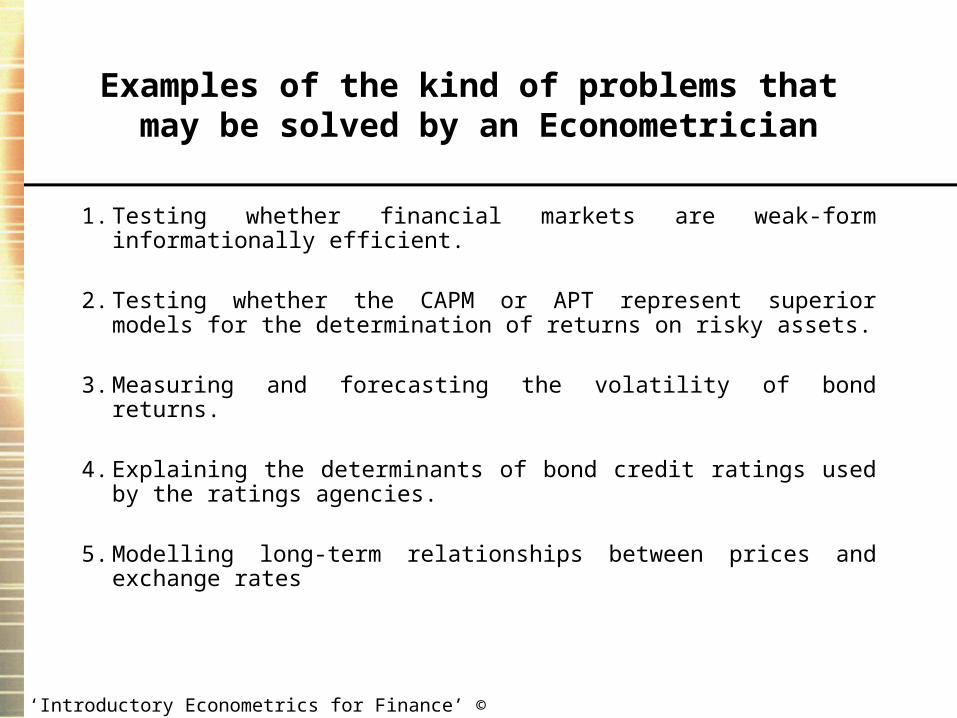
Examples of the kind of problems that may be solved by an Econometrician
1. Testing whether financial markets are weak-form informationally efficient.
2. Testing whether the CAPM or APT represent superior models for the determination of returns on risky assets.
3. Measuring and forecasting the volatility of bond returns.
4. Explaining the determinants of bond credit ratings used by the ratings agencies.
5. Modelling long-term relationships between prices and exchange rates
‘Introductory Econometrics for Finance’ © Chris Brooks 2008
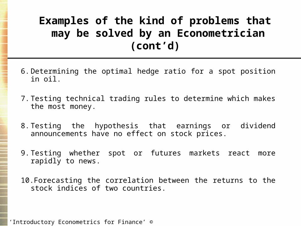
Examples of the kind of problems that may be solved by an Econometrician (cont’d)
6. Determining the optimal hedge ratio for a spot position in oil.
7. Testing technical trading rules to determine which makes the most money.
8. Testing the hypothesis that earnings or dividend announcements have no effect on stock prices.
9. Testing whether spot or futures markets react more rapidly to news.
10.Forecasting the correlation between the returns to the stock indices of two countries.
‘Introductory Econometrics for Finance’ © Chris Brooks 2008
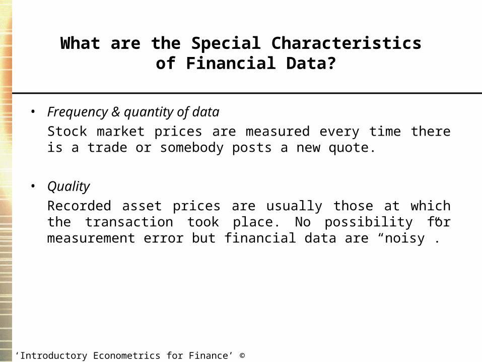
• Frequency & quantity of data
Stock market prices are measured every time there is a trade or somebody posts a new quote.
• Quality
Recorded asset prices are usually those at which the transaction took place. No possibility for measurement error but financial data are “noisy”.
What are the Special Characteristics of Financial Data?
‘Introductory Econometrics for Finance’ © Chris Brooks 2008
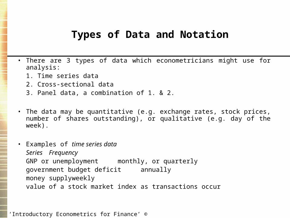
Types of Data and Notation
• There are 3 types of data which econometricians might use for analysis:1. Time series data2. Cross-sectional data3. Panel data, a combination of 1. & 2.
• The data may be quantitative (e.g. exchange rates, stock prices, number of shares outstanding), or qualitative (e.g. day of the week).
• Examples of time series dataSeries FrequencyGNP or unemployment monthly, or quarterlygovernment budget deficit annuallymoney supply weeklyvalue of a stock market index as transactions occur
‘Introductory Econometrics for Finance’ © Chris Brooks 2008
Time Series versus Cross-sectional Data
• Examples of Problems that Could be Tackled Using a Time Series Regression
- How the value of a country’s stock index has varied with that country’s
macroeconomic fundamentals.
- How the value of a company’s stock price has varied when it announced the
value of its dividend payment.
- The effect on a country’s currency of an increase in its interest rate
– How the value of a country’s stock index has varied with that country’s macroeconomic fundamentals.
– How a company’s stock returns has varied when it announced the value of its dividend payment.
– The effect on a country’s currency of an increase in its interest rate
• Cross-sectional data are data on one or more variables collected at a single point in time, e.g.
- A poll of usage of internet stock broking services
- Cross-section of stock returns on the New York Stock Exchange
- A sample of bond credit ratings for UK banks• The relationship between company size and the return to
investing in its shares
• The relationship between a country’s GDP level and the probability that the government will default on its sovereign debt
‘Introductory Econometrics for Finance’ © Chris Brooks 2008
‘Introductory Econometrics for Finance’ © Chris Brooks 2008
Cross-sectional and Panel Data
• Examples of Problems that Could be Tackled Using a Cross-Sectional Regression
- The relationship between company size and the return to investing in its shares
- The relationship between a country’s GDP level and the probability that the
government will default on its sovereign debt.
• Panel Data has the dimensions of both time series and cross-sections, e.g. the daily prices of a number of blue chip stocks over two years.
• It is common to denote each observation by the letter t and the total number of observations by T for time series data, and to to denote each observation by the letter i and the total number of observations by N for cross-sectional data.
‘Introductory Econometrics for Finance’ © Chris Brooks 2008
Continuous and Discrete Data
• Continuous data can take on any value and are not confined to take specific numbers.
• Their values are limited only by precision. – For example, the rental yield on a property could be 6.2%, 6.24%, or 6.238%.
• On the other hand, discrete data can only take on certain values, which are usually integers– For instance, the number of people in a particular underground carriage or the number
of shares traded during a day.
• They do not necessarily have to be integers (whole numbers) though, and are often defined to be count numbers. – For example, until recently when they became ‘decimalised’, many financial asset
prices were quoted to the nearest 1/16 or 1/32 of a dollar.
‘Introductory Econometrics for Finance’ © Chris Brooks 2008
Cardinal, Ordinal and Nominal Numbers
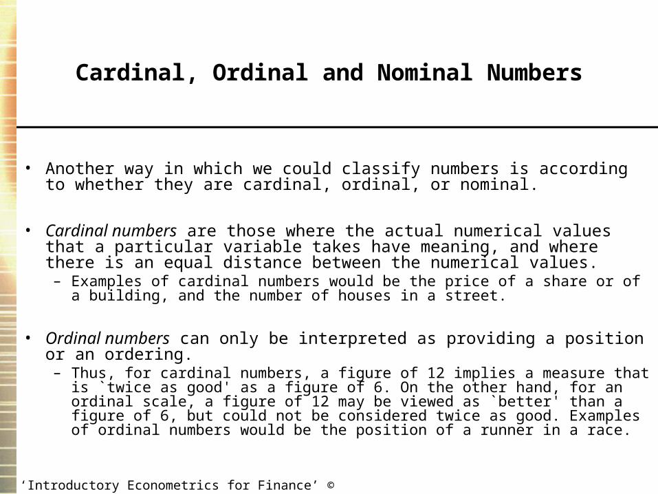
• Another way in which we could classify numbers is according to whether they are cardinal, ordinal, or nominal.
• Cardinal numbers are those where the actual numerical values that a particular variable takes have meaning, and where there is an equal distance between the numerical values. – Examples of cardinal numbers would be the price of a share or of a building, and the
number of houses in a street.
• Ordinal numbers can only be interpreted as providing a position or an ordering. – Thus, for cardinal numbers, a figure of 12 implies a measure that is `twice as good' as
a figure of 6. On the other hand, for an ordinal scale, a figure of 12 may be viewed as `better' than a figure of 6, but could not be considered twice as good. Examples of ordinal numbers would be the position of a runner in a race.
‘Introductory Econometrics for Finance’ © Chris Brooks 2008
Cardinal, Ordinal and Nominal Numbers (Cont’d)
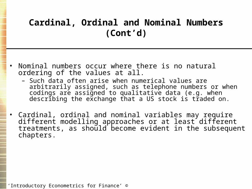
• Nominal numbers occur where there is no natural ordering of the values at all. – Such data often arise when numerical values are arbitrarily assigned, such as telephone
numbers or when codings are assigned to qualitative data (e.g. when describing the exchange that a US stock is traded on.
• Cardinal, ordinal and nominal variables may require different modelling approaches or at least different treatments, as should become evident in the subsequent chapters.
15
Econometrics versus Financial Econometrics
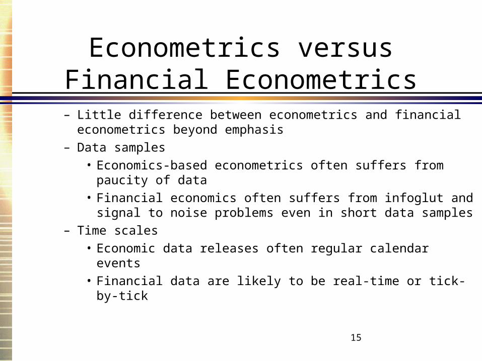
– Little difference between econometrics and financial econometrics beyond emphasis
– Data samples• Economics-based econometrics often suffers from paucity of data
• Financial economics often suffers from infoglut and signal to noise problems even in short data samples
– Time scales• Economic data releases often regular calendar events
• Financial data are likely to be real-time or tick-by-tick
16
Economic Data versus Financial Data
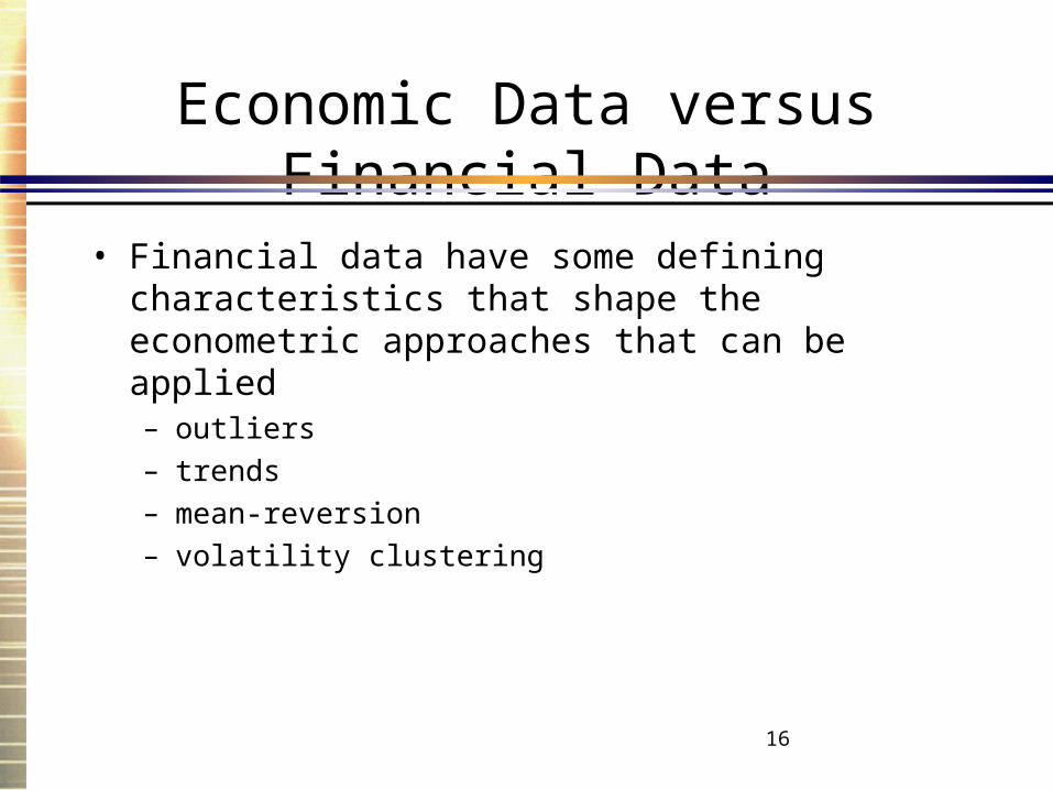
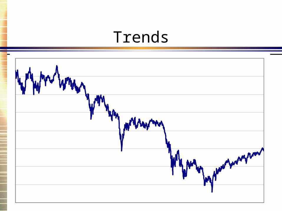
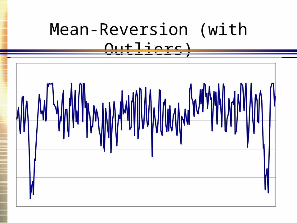
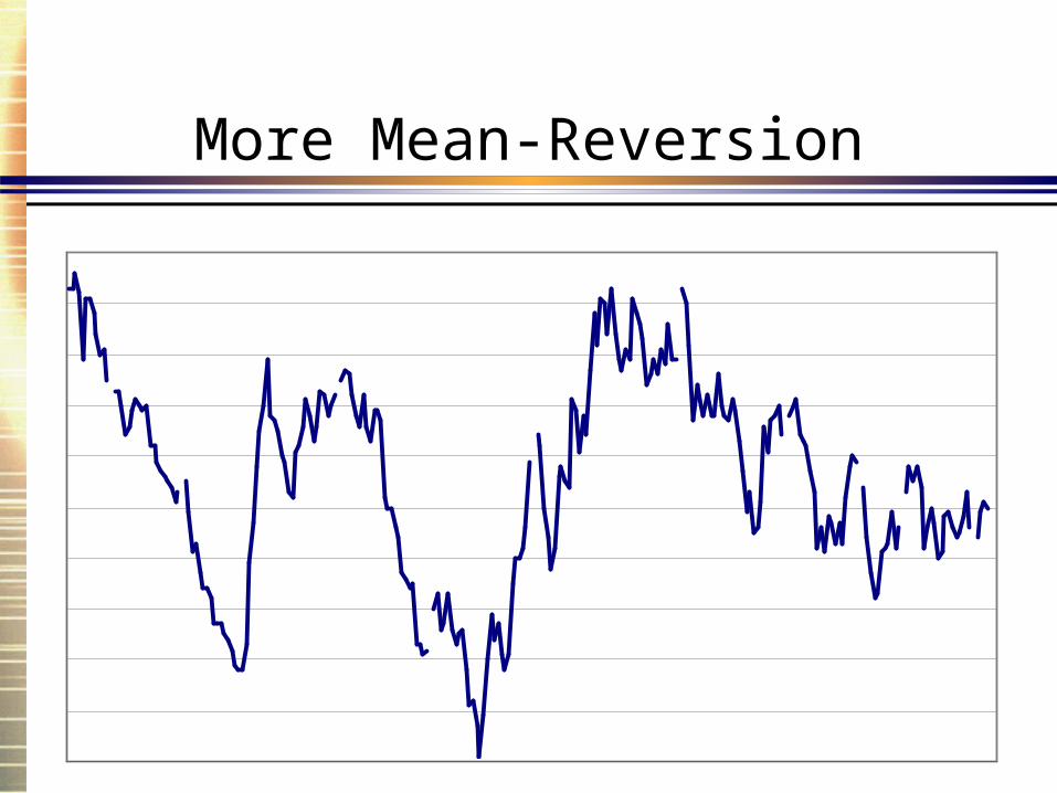
• Financial data have some defining characteristics that shape the econometric approaches that can be applied– outliers– trends– mean-reversion– volatility clustering
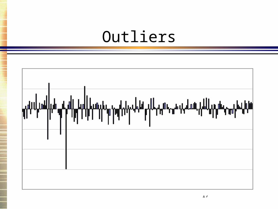
17
Outliers
18
Trends
19
Mean-Reversion (with Outliers)
20
More Mean-Reversion
21
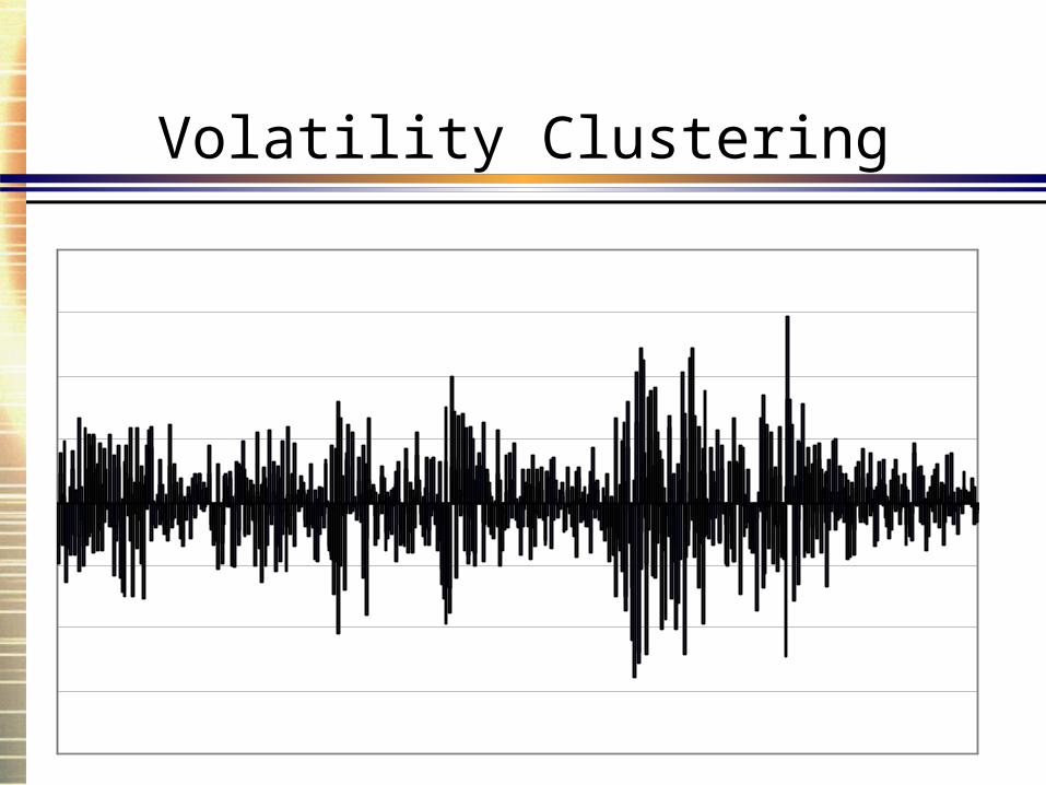
Volatility Clustering
22
Basic Data Analysis
• All pieces of empirical work should begin with some basic data analysis– Eyeball the data– Summarize the properties of the data series– Examine the relationship between data series
• Most powerful analytic tools are your eyes and your common sense– Computers still suffer from “Garbage in - garbage
out”
23
Basic Data Analysis
• Eyeballing the data helps establish presence of – trends versus mean reversion– volatility clusters– key observations
• outliers
– data errors?
• turning points
• regime changes
24
Basic Data Analysis
• Summary statistics– Average level of variable
• Mean, median, mode
– Variability around this central tendency• Standard deviations, variances, maxima/minima
– Distribution of data• Skewness, kurtosis
– Number of observations, number of missing observations
25
Basic Data Analysis
• Since we are usually concerned with explaining one variable using another– “trading volume depends positively on volatility”
• relationships between variables are important– cross-plots, multiple time-series plots– correlations (covariances)– multi-collinearity
26
Basic Data Manipulations
• Taking natural logarithms• Calculating returns• Seasonally adjusting• De-meaning• De-trending• Lagging and leading
‘Introductory Econometrics for Finance’ © Chris Brooks 2008
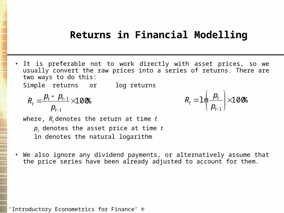
• It is preferable not to work directly with asset prices, so we usually convert the raw prices into a series of returns. There are two ways to do this:Simple returns or log returns
where, Rt denotes the return at time t
pt denotes the asset price at time t ln denotes the natural logarithm
• We also ignore any dividend payments, or alternatively assume that the price series have been already adjusted to account for them.
Returns in Financial Modelling
%1001
1
t
ttt p
ppR %100ln
1
t
tt p
pR
‘Introductory Econometrics for Finance’ © Chris Brooks 2008
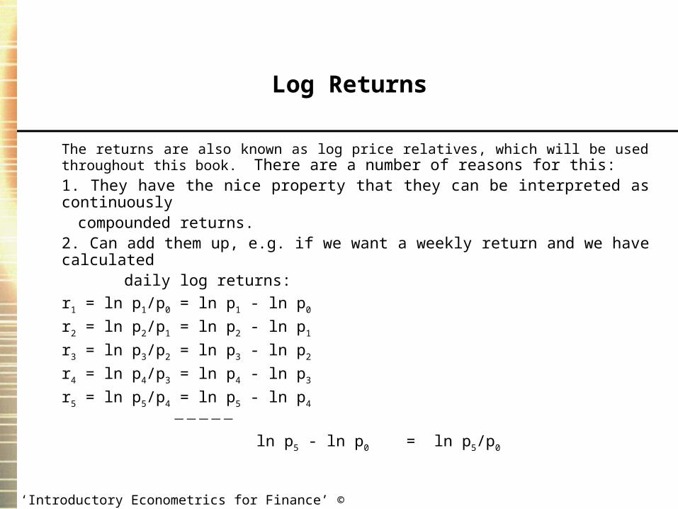
The returns are also known as log price relatives, which will be used throughout this book. There are a number of reasons for this:1. They have the nice property that they can be interpreted as continuously
compounded returns.2. Can add them up, e.g. if we want a weekly return and we have calculated
daily log returns:
r1 = ln p1/p0 = ln p1 - ln p0
r2 = ln p2/p1 = ln p2 - ln p1
r3 = ln p3/p2 = ln p3 - ln p2
r4 = ln p4/p3 = ln p4 - ln p3
r5 = ln p5/p4 = ln p5 - ln p4
ln p5 - ln p0 = ln p5/p0
Log Returns
‘Introductory Econometrics for Finance’ © Chris Brooks 2008
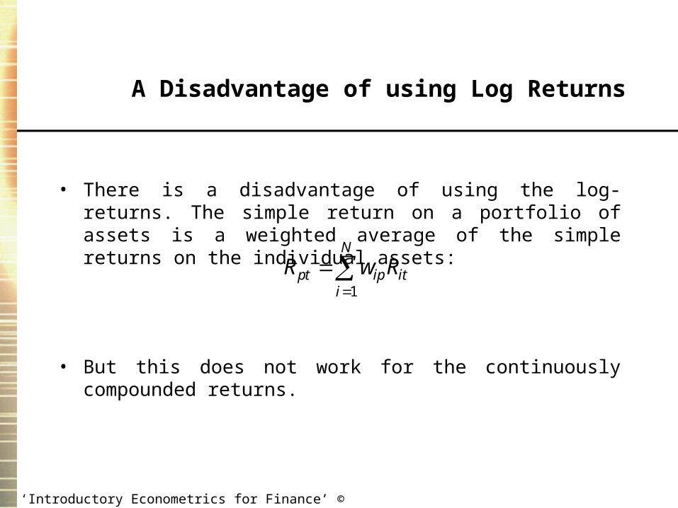
• There is a disadvantage of using the log-returns. The simple return on a portfolio of assets is a weighted average of the simple returns on the individual assets:
• But this does not work for the continuously compounded returns.
A Disadvantage of using Log Returns
R w Rpt ip iti
N
1
‘Introductory Econometrics for Finance’ © Chris Brooks 2008
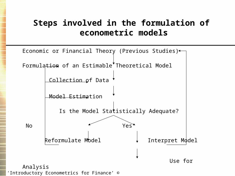
Steps involved in the formulation of econometric models
Economic or Financial Theory (Previous Studies)
Formulation of an Estimable Theoretical Model
Collection of Data
Model Estimation
Is the Model Statistically Adequate?
No Yes
Reformulate Model Interpret Model
Use for Analysis
‘Introductory Econometrics for Finance’ © Chris Brooks 2008
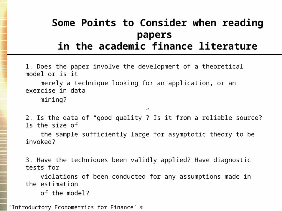
1. Does the paper involve the development of a theoretical model or is it
merely a technique looking for an application, or an exercise in data
mining?
2. Is the data of “good quality”? Is it from a reliable source? Is the size of
the sample sufficiently large for asymptotic theory to be invoked?
3. Have the techniques been validly applied? Have diagnostic tests for
violations of been conducted for any assumptions made in the estimation
of the model?
Some Points to Consider when reading papers in the academic finance literature
‘Introductory Econometrics for Finance’ © Chris Brooks 2008
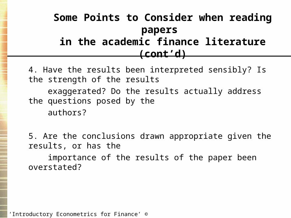
4. Have the results been interpreted sensibly? Is the strength of the results
exaggerated? Do the results actually address the questions posed by the
authors?
5. Are the conclusions drawn appropriate given the results, or has the
importance of the results of the paper been overstated?
Some Points to Consider when reading papers in the academic finance literature (cont’d)


