438 CHAPTER 11. MULTIPLE REGRESSION AND CORRELATION Chapter 9 introduced regression modeling of the relationship between two quantitative variables. Multivariate relationships require more complex models, containing several explanatory variables. Some of these may be predictors of theoretical interest, and some may be control variables. To predict Y = college GPA, for example, it is sensible to use several predictors in the same model. Possibilities include X 1 = high school GPA, X 2 = math college entrance exam score, X 3 = verbal college entrance exam score, and X 4 = rating by high school guidance counselor. This chapter presents models for the relationship between a response variable Y and a collection of explanatory variables. A multivariable model provides better predictions of Y than does a model with a single explanatory variable. Such a model also can analyze relationships between variables while controlling for other variables. This is important because Chapter 10 showed that after controlling for a variable, an association can appear quite different from when the variable is ignored. Thus, this model provides information not available with simple models that analyze only two variables at a time. Sections 11.1 and 11.2 extend the regression model to a multiple regression model that can have multiple explanatory variables. Section 11.3 defines correlation and r-squared measures that describe association between Y and a set of explanatory variables. Section 11.4 presents inference procedures for multiple regression. Section 11.5 shows how to allow statistical interaction in the model, and Section 11.6 presents a test of whether a complex model provides a better fit than a simpler model. The final two sections introduce measures that summarize the association between the response variable and an explanatory variable while controlling other variables. 11.1 The Multiple Regression Model Chapter 9 modeled the relationship between the explanatory variable X and the mean of the response variable Y by the straight-line (linear) equation E(Y )= α + βx. We refer to this model containing a single predictor as a bivariate model, because it contains only two variables. The Multiple Regression Function Suppose there are two explanatory variables, denoted by X 1 and X 2 . As in earlier chapters, we use lower-case letters to denote observations or particular values of the variables. The bivariate regression function generalizes to the multiple regression function E(Y )= α + β 1 x 1 + β 2 x 2 . In this equation, α, β 1 , and β 2 are parameters discussed below. For particular values of x 1 and x 2 , the equation specifies the population mean of Y for all subjects with those values of x 1 and x 2 . When there are additional explanatory variables, each has a βx term, for example E(Y )= α + β 1 x 1 + β 2 x 2 + β 3 x 3 + β 4 x 4 with four predictors. The multiple regression function is more difficult to portray graphically than the bivariate regression function. With two explanatory variables, the x 1 and x 2 axes are
Transcript
438 CHAPTER 11. MULTIPLE REGRESSION AND CORRELATION
Chapter 9 introduced regression modeling of the relationship between two quantitative
variables. Multivariate relationships require more complex models, containing several
explanatory variables. Some of these may be predictors of theoretical interest, and
some may be control variables.
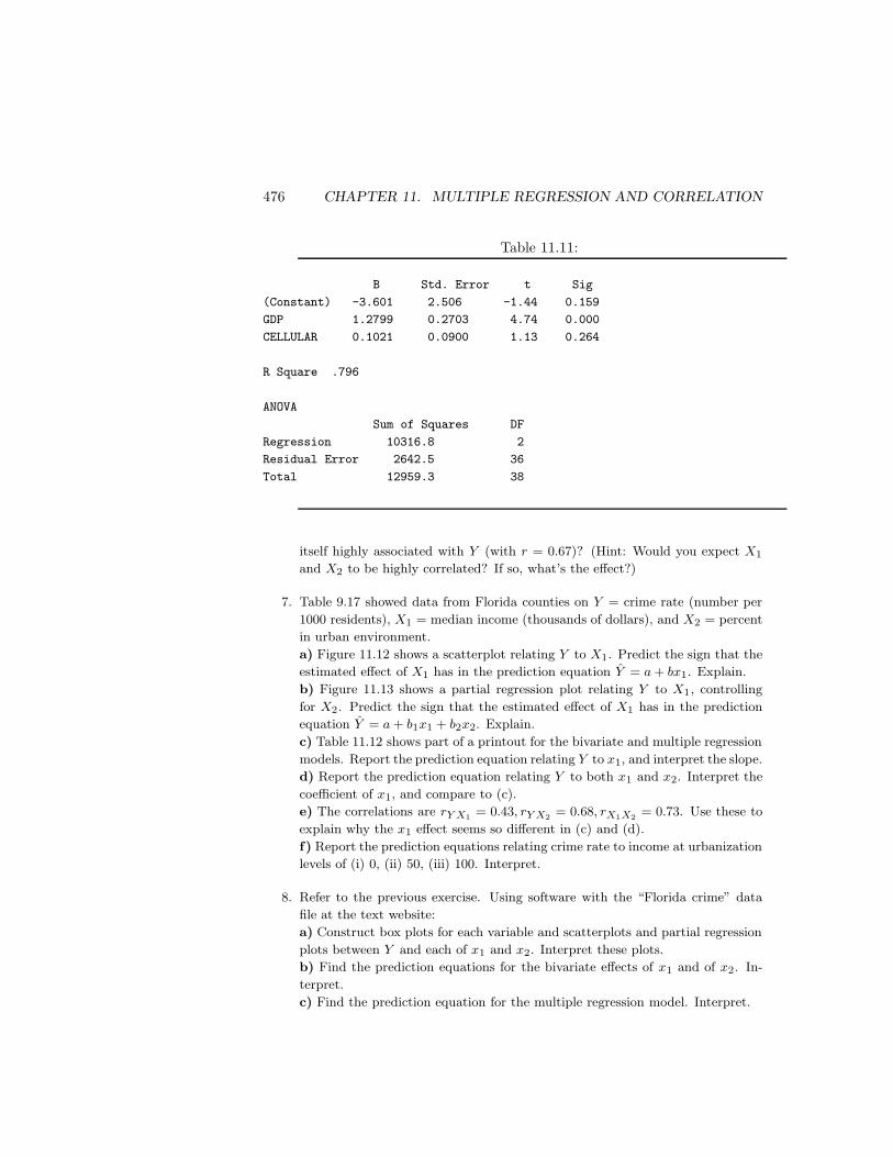
To predict Y = college GPA, for example, it is sensible to use several predictors
in the same model. Possibilities include X1 = high school GPA, X2 = math college
entrance exam score, X3 = verbal college entrance exam score, and X4 = rating by
high school guidance counselor. This chapter presents models for the relationship
between a response variable Y and a collection of explanatory variables.
A multivariable model provides better predictions of Y than does a model with
a single explanatory variable. Such a model also can analyze relationships between
variables while controlling for other variables. This is important because Chapter 10
showed that after controlling for a variable, an association can appear quite different
from when the variable is ignored. Thus, this model provides information not available
with simple models that analyze only two variables at a time.
Sections 11.1 and 11.2 extend the regression model to a multiple regression
model that can have multiple explanatory variables. Section 11.3 defines correlation
and r-squared measures that describe association between Y and a set of explanatory
variables. Section 11.4 presents inference procedures for multiple regression. Section
11.5 shows how to allow statistical interaction in the model, and Section 11.6 presents
a test of whether a complex model provides a better fit than a simpler model. The
final two sections introduce measures that summarize the association between the
response variable and an explanatory variable while controlling other variables.
11.1 The Multiple Regression Model
Chapter 9 modeled the relationship between the explanatory variable X and the mean
of the response variable Y by the straight-line (linear) equation E(Y ) = α + βx. We
refer to this model containing a single predictor as a bivariate model, because it
contains only two variables.
The Multiple Regression Function
Suppose there are two explanatory variables, denoted by X1 and X2. As in earlier
chapters, we use lower-case letters to denote observations or particular values of the
variables. The bivariate regression function generalizes to the multiple regression
function
E(Y ) = α + β1x1 + β2x2.
In this equation, α, β1, and β2 are parameters discussed below. For particular values
of x1 and x2, the equation specifies the population mean of Y for all subjects with
those values of x1 and x2. When there are additional explanatory variables, each has
a βx term, for example E(Y ) = α + β1x1 + β2x2 + β3x3 + β4x4 with four predictors.
The multiple regression function is more difficult to portray graphically than the
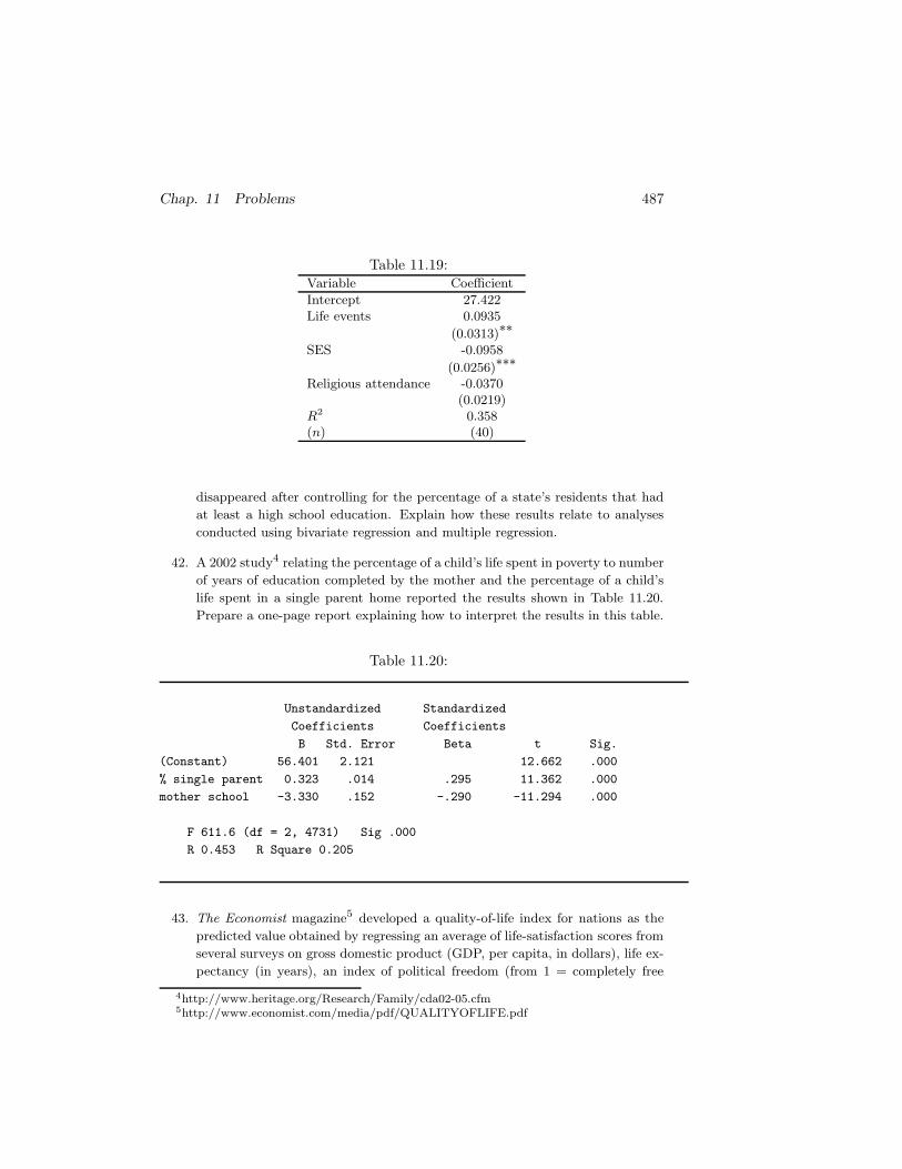
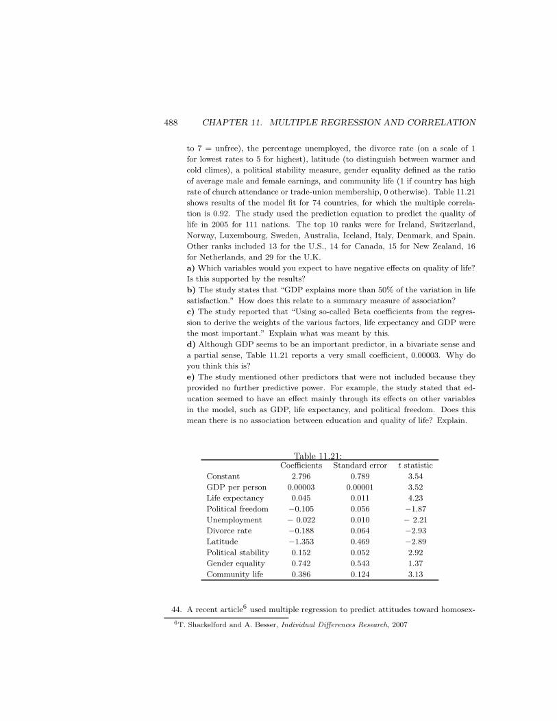
bivariate regression function. With two explanatory variables, the x1 and x2 axes are
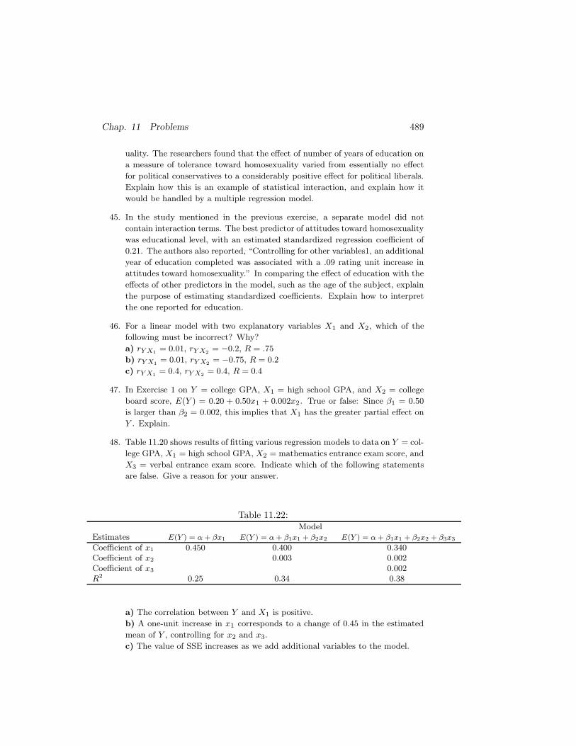
11.1. THE MULTIPLE REGRESSION MODEL 439
Figure 11.1: Graphical Depiction of a Multiple Regression Function with TwoExplanatory Variables
((Fig. 11.1 in 3e))
perpendicular but lie in a horizontal plane and the Y axis is vertical and perpendicular
to both the x1 and x2 axes. The equation E(Y ) = α + β1x1 + β2x2 traces a plane (a
flat surface) cutting through three-dimensional space, as Figure 11.1 portrays.
The simplest interpretation treats all but one explanatory variable as control vari-
ables and fixes them at particular levels. This leaves an equation relating the mean
of Y to the remaining explanatory variable.
Example 11.1 Do Higher Levels of Education Cause Higher Crime Rates?
Exercise 39 in Chapter 9 contains recent data on several variables for the 67
counties in the state of Florida. For each county, let Y = crime rate (annual number
of crimes per 1000 population), X1 = education (percentage of adult residents having
at least a high school education), and X2 = urbanization (percentage living in an
urban environment).
The bivariate relationship between crime rate and education is approximated by
E(Y ) = −51.3 + 1.5x1. Surprisingly, the association is moderately positive, the cor-
relation being r = 0.47. As the percentage of county residents having at least a high
school education increases, so does the crime rate.
A closer look at the data reveals strong positive associations between crime rate
and urbanization (r = 0.68) and between education and urbanization (r = 0.79).
This suggests that the association between crime rate and education may be spurious.
Perhaps urbanization is a common causal factor. See Figure 11.2. As urbanization
increases, both crime rate and education increase, resulting in a positive correlation
between crime rate and education.
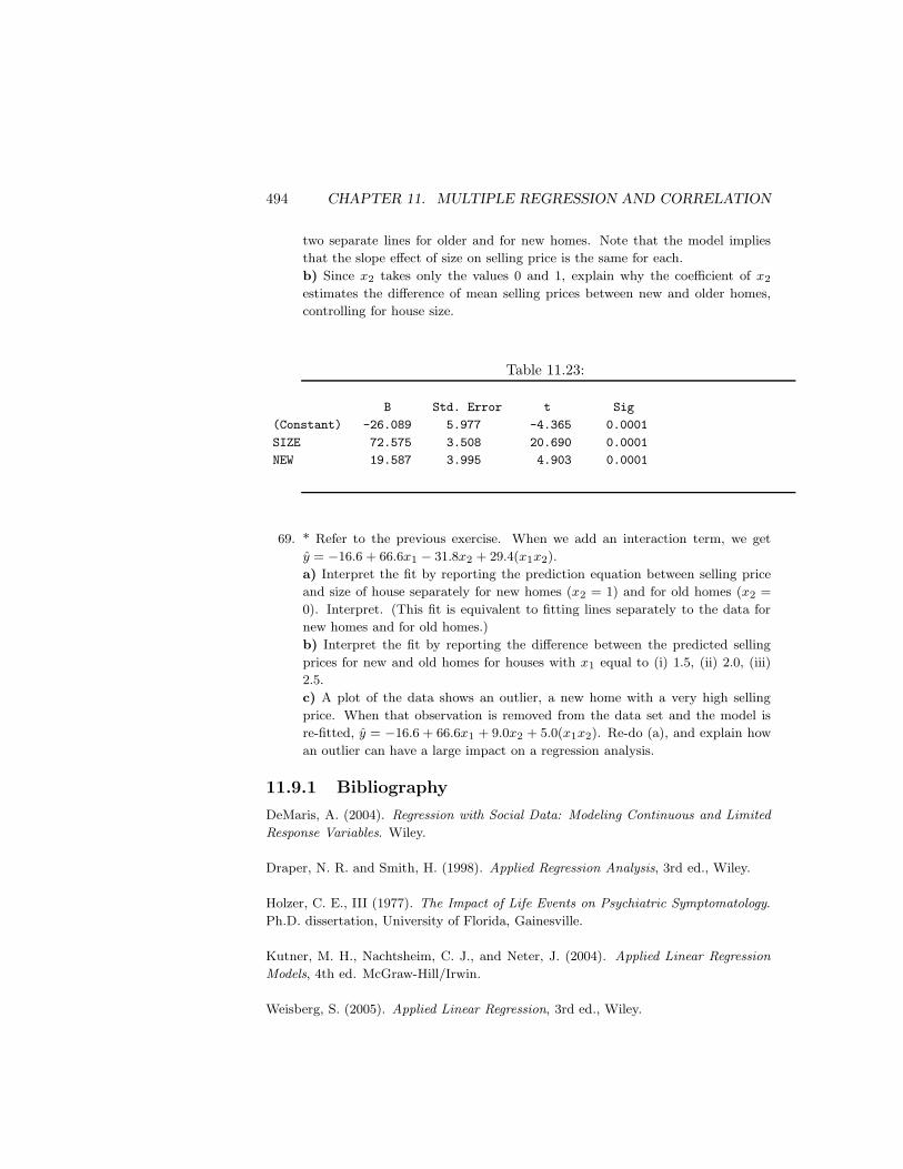
The relation between crime rate and both predictors considered together is ap-
proximated by the multiple regression function
E(Y ) = 58.9 − 0.6x1 + 0.7x2.
For instance, the expected crime rate for a county at the mean levels of education
Figure 11.2: The Positive Association Between Crime Rate and Education MayBe Spurious, Explained by the Effects of Urbanization on Each
((Fig. 11.2 in 3e))
440 CHAPTER 11. MULTIPLE REGRESSION AND CORRELATION
(x1 = 70) and urbanization (x2 = 50) is E(Y ) = 58.9− 0.6(70) + 0.7(50) = 52 annual
crimes per 1000 population.
Let’s study the effect of x1, controlling for x2. We first set x2 at its mean level of
50. Then, the relationship between crime rate and education is
Figure 11.3 plots this line. Controlling for x2 by fixing it at 50, the relationship be-
tween crime rate and education is negative, rather than positive. The slope decreased
and changed sign from 1.5 in the bivariate relationship to −0.6. At this fixed level of
urbanization, a negative relationship exists between education and crime rate. We use
the term partial regression equation to distinguish the equation E(Y ) = 93.9 − 0.6x1
from the regression equation E(Y ) = −51.3 + 1.5x1 for the bivariate relationship
between Y and x1. The partial regression equation refers to part of the potential
observations, in this case counties having x2 = 50.
Figure 11.3: Partial Relationships Between E(Y ) and x1 for the Multiple Re-gression Equation E(Y ) = 58.9− 0.6x1 + 0.7x2. These partial regression equa-tions fix x2 to equal 50 or 40.
((Fig. 11.3 in 3e))
Next we fix x2 at a different level, say x2 = 40 instead of 50. Then, you can check
that E(Y ) = 86.9 − 0.6x1. Thus, decreasing x2 by 10 units shifts the partial line
relating Y to x1 downward by 10β2 = 7.0 units (see Figure 11.3). The slope of −0.6
for the partial relationship remains the same, so the line is parallel to the original one.
Setting x2 at a variety of values yields a collection of parallel lines, each having slope
β1 = −0.6.
Similarly, setting x1 at a variety of values yields a collection of parallel lines,
each having slope 0.7, relating the mean of Y to x2. In other words, controlling for
education, the slope of the partial relationship between crime rate and urbanization
is β2 = 0.7.
In summary, education has an overall positive effect on crime rate, but it has
a negative effect when controlling for urbanization. The partial association has the
opposite direction from the bivariate association. This is called Simpson’s para-
dox. Figure 11.4 illustrates how this happens. It shows the scatterplot relating crime
rate to education, portraying the overall positive association between these variables.
The diagram circles the 19 counties that are highest in urbanization. That subset of
points for which urbanization is nearly constant has a negative trend between crime
rate and education. The high positive association between education and urbanization
is reflected by the fact that most of the highlighted observations that are highest on
urbanization also have high values on education.
2
11.1. THE MULTIPLE REGRESSION MODEL 441
Figure 11.4: Scatterplot Relating Crime Rate and Education. The circled pointsare the counties highest on Urbanization. A regression line fitting the circledpoints has negative slope, even though the regression line passing through all
the points has positive slope (Simpson’s paradox).
((Fig. 11.4 in 3e))
Interpretation of Regression Coefficients
We have seen that for a fixed value of x2, the equation E(Y ) = α + β1x1 + β2x2
simplifies to a straight-line equation in x1 with slope β1. The slope is the same for
each fixed value of x2. When we fix the value of x2, we are holding it constant: We are
controlling for x2. That’s the basis of the major difference between the interpretation
of slopes in multiple regression and in bivariate regression:
• In multiple regression, a slope describes the effect of an explanatory variable
while controlling effects of the other explanatory variables in the model.
• Bivariate regression has only a single explanatory variable. So, a slope in bi-
variate regression describes the effect of that variable while ignoring all other
possible explanatory variables.
The parameter β1 measures the partial effect of x1 on Y , that is, the effect of a
one-unit increase in x1, holding x2 constant. The partial effect of x2 on Y , holding
x1 constant, has slope β2. Similarly, for the multiple regression model with several
predictors, the beta coefficient of a predictor describes the change in the mean of Y for
a one-unit increase in that predictor, controlling for the other variables in the model.
The parameter α represents the mean of Y when each explanatory variable equals 0.
The parameters β1, β2, . . . are called partial regression coefficients. The
adjective partial distinguishes these parameters from the regression coefficient β in
the bivariate model E(Y ) = α + βx, which ignores rather than controls effects of
other explanatory variables.
This multiple regression model assumes that the slope of the partial relationship
between Y and each predictor is identical for all combinations of values of the other
explanatory variables. This means that the model is appropriate when there is no
statistical interaction, in the sense of Section 10.3. If the true partial slope between
Y and x1 is very different at x2 = 50 than at x2 = 40, for example, we need a more
complex model. Section 11.5 will show this model.
A partial slope in a multiple regression model usually differs from the slope in the
bivariate model for that predictor, but it need not. With two predictors, the partial
slopes and bivariate slopes are equal if the correlation between X1 and X2 equals 0.
When X1 and X2 are independent causes of Y , the effect of X1 on Y does not change
when we control for X2.
442 CHAPTER 11. MULTIPLE REGRESSION AND CORRELATION
Prediction Equation and Residuals
Corresponding to the multiple regression equation, software finds a prediction equation
by estimating the model parameters using sample data. For simplicity of notation, so
far we’ve used just two predictors. In general, let k denote the number of predictors.
Notation for Prediction Equation
The prediction equation that estimates the multiple regression equation E(Y ) =
α + β1x1 + β2x2 + · · · + βkxk is denoted by y = a + b1x1 + b2x2 + · · · + bkxk.
For multiple regression, it is almost imperative to use computer software to find the
prediction equation. The calculation formulas are complex and are not shown in this
text.
We get the predicted value of Y for a subject by substituting the x-values for that
subject into the prediction equation. Like the bivariate model, the multiple regression
model has residuals that measure prediction errors. For a subject with predicted
response y and observed response y, the residual is y − y. The next section shows an
example.
The sum of squared errors (SSE),
SSE =∑
(y − y)2
summarizes the closeness of fit of the prediction equation to the response data. Most
software calls SSE the residual sum of squares. The formula for SSE is the same
as in Chapter 9. The only difference is that the predicted value y results from using
several explanatory variables instead of just a single predictor.
The parameter estimates in the prediction equation satisfy the least squares
criterion: The prediction equation has the smallest SSE value of all possible equations
of form Y = a + b1x1 + · · · + bkxk.
11.2 Example with Multiple Regression Com-
puter Output
We illustrate the methods of this chapter with the data introduced in the following
example:
Example 11.2 Multiple Regression for Mental Health Study
A study in Alachua County, Florida, investigated the relationship between certain
mental health indices and several explanatory variables. Primary interest focused on
an index of mental impairment, which incorporates various dimensions of psychiatric
symptoms, including aspects of anxiety and depression. This measure, which is the
response variable Y , ranged from 17 to 41 in the sample. Higher scores indicate
greater psychiatric impairment.
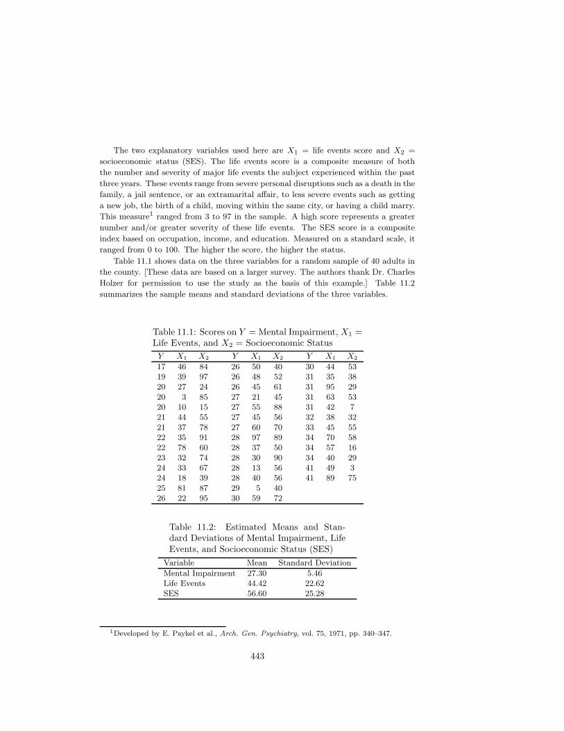
The two explanatory variables used here are X1 = life events score and X2 =
socioeconomic status (SES). The life events score is a composite measure of both
the number and severity of major life events the subject experienced within the past
three years. These events range from severe personal disruptions such as a death in the
family, a jail sentence, or an extramarital affair, to less severe events such as getting
a new job, the birth of a child, moving within the same city, or having a child marry.
This measure1 ranged from 3 to 97 in the sample. A high score represents a greater
number and/or greater severity of these life events. The SES score is a composite
index based on occupation, income, and education. Measured on a standard scale, it
ranged from 0 to 100. The higher the score, the higher the status.
Table 11.1 shows data on the three variables for a random sample of 40 adults in
the county. [These data are based on a larger survey. The authors thank Dr. Charles
Holzer for permission to use the study as the basis of this example.] Table 11.2
summarizes the sample means and standard deviations of the three variables.
Table 11.1: Scores on Y = Mental Impairment, X1 =Life Events, and X2 = Socioeconomic Status
The correlation r and its square describe strength of linear association for bivariate
relationships. This section presents analogous measures for the multiple regression
model. They describe the strength of association between Y and the set of explanatory
variables acting together as predictors in the model.
The Multiple Correlation
The explanatory variables collectively are strongly associated with Y if the observed y-
values correlate highly with the y-values from the prediction equation. The correlation
between the observed and predicted values summarizes this association.
Multiple Correlation
The multiple correlation for a regression model is the correlation between the ob-
served y-values and the predicted y-values.
For each subject, the prediction equation provides a predicted value y. So, each
subject has a y-value and a y-value. For example, above we saw that the first subject
in the sample had y = 17 and y = 24.8. For the first three subjects in Table 11.1, the
observed and predicted y-values are:
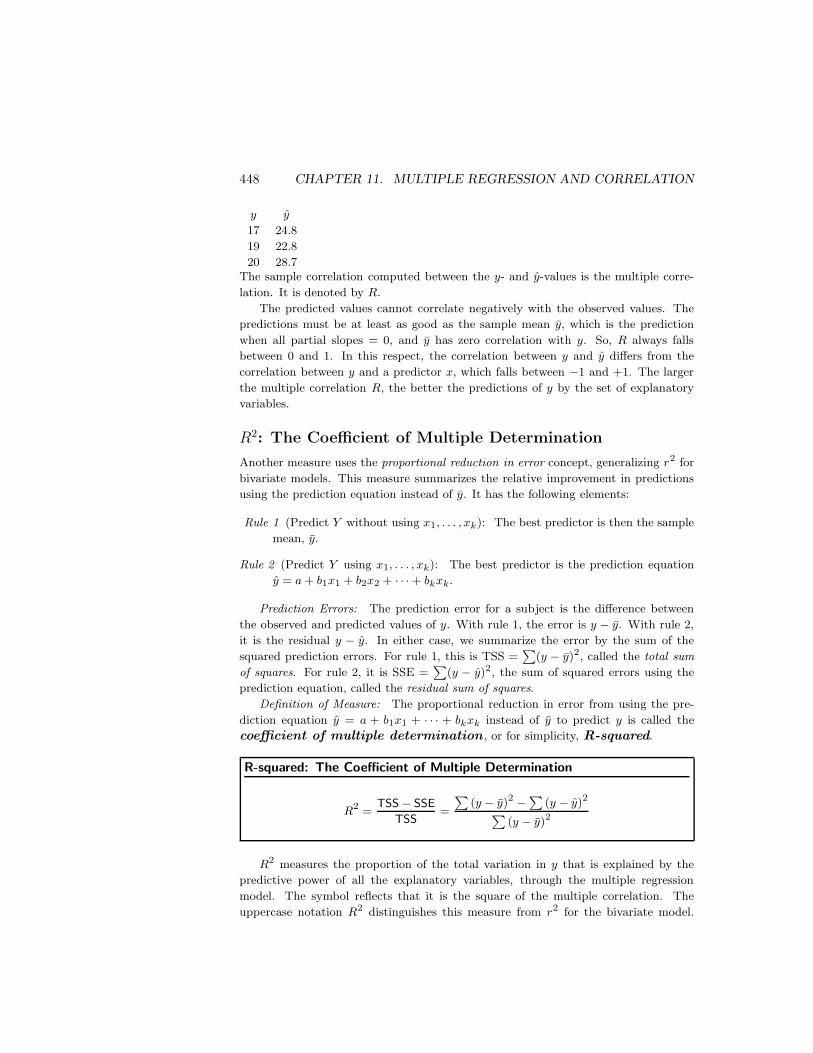
448 CHAPTER 11. MULTIPLE REGRESSION AND CORRELATION
y y
17 24.8
19 22.8
20 28.7The sample correlation computed between the y- and y-values is the multiple corre-
lation. It is denoted by R.
The predicted values cannot correlate negatively with the observed values. The
predictions must be at least as good as the sample mean y, which is the prediction
when all partial slopes = 0, and y has zero correlation with y. So, R always falls
between 0 and 1. In this respect, the correlation between y and y differs from the
correlation between y and a predictor x, which falls between −1 and +1. The larger
the multiple correlation R, the better the predictions of y by the set of explanatory
variables.
R2: The Coefficient of Multiple Determination
Another measure uses the proportional reduction in error concept, generalizing r2 for
bivariate models. This measure summarizes the relative improvement in predictions
using the prediction equation instead of y. It has the following elements:
Rule 1 (Predict Y without using x1, . . . , xk): The best predictor is then the sample
mean, y.
Rule 2 (Predict Y using x1, . . . , xk): The best predictor is the prediction equation
y = a + b1x1 + b2x2 + · · · + bkxk.
Prediction Errors: The prediction error for a subject is the difference between
the observed and predicted values of y. With rule 1, the error is y − y. With rule 2,
it is the residual y − y. In either case, we summarize the error by the sum of the
squared prediction errors. For rule 1, this is TSS =∑
(y − y)2, called the total sum
of squares. For rule 2, it is SSE =∑
(y − y)2, the sum of squared errors using the
prediction equation, called the residual sum of squares.
Definition of Measure: The proportional reduction in error from using the pre-
diction equation y = a + b1x1 + · · · + bkxk instead of y to predict y is called the
coefficient of multiple determination , or for simplicity, R-squared.
R-squared: The Coefficient of Multiple Determination
R2 =TSS − SSE
TSS=
∑
(y − y)2 −∑
(y − y)2
∑
(y − y)2
R2 measures the proportion of the total variation in y that is explained by the
predictive power of all the explanatory variables, through the multiple regression
model. The symbol reflects that it is the square of the multiple correlation. The
uppercase notation R2 distinguishes this measure from r2 for the bivariate model.
11.3. MULTIPLE CORRELATION AND R2 449
Their formulas are identical, and r2 is the special case of R2 applied to a regression
model with one explanatory variable. For the multiple regression model to be useful
for prediction, it should provide improved predictions relative not only to y but also
to the separate bivariate models for y and each explanatory variable.
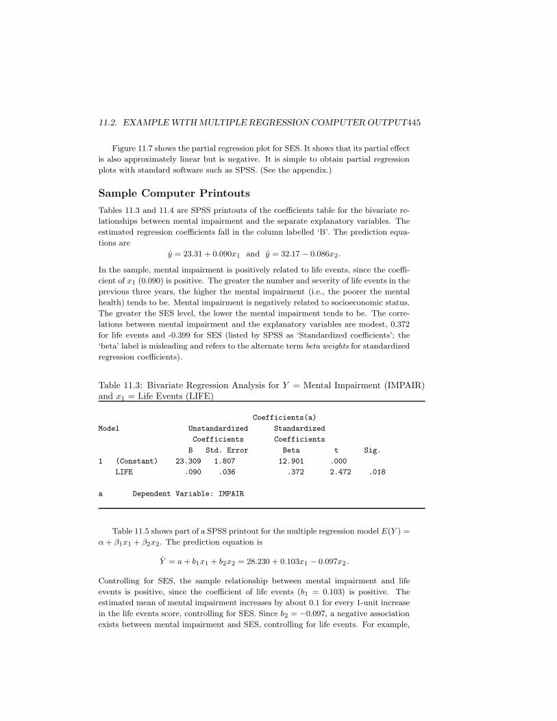
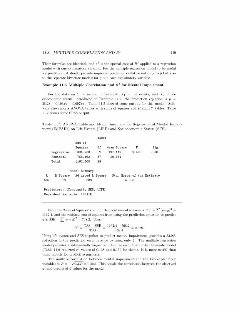
Example 11.3 Multiple Correlation and R2 for Mental Impairment
For the data on Y = mental impairment, X1 = life events, and X2 = so-
cioeconomic status, introduced in Example 11.2, the prediction equation is y =
28.23 + 0.103x1 − 0.097x2. Table 11.5 showed some output for this model. Soft-
ware also reports ANOVA tables with sums of squares and R and R2 tables. Table
11.7 shows some SPSS output.
Table 11.7: ANOVA Table and Model Summary for Regression of Mental Impair-ment (IMPAIR) on Life Events (LIFE) and Socioeconomic Status (SES)
ANOVA
Sum of
Squares df Mean Square F Sig.
Regression 394.238 2 197.119 9.495 .000
Residual 768.162 37 20.761
Total 1162.400 39
Model Summary
R R Square Adjusted R Square Std. Error of the Estimate
.582 .339 .303 4.556
Predictors: (Constant), SES, LIFE
Dependent Variable: IMPAIR
From the ‘Sum of Squares’ column, the total sum of squares is TSS =∑
(y− y)2 =
1162.4, and the residual sum of squares from using the prediction equation to predict
y is SSE =∑
(y − y)2 = 768.2. Thus,
R2 =TSS − SSE
TSS=
1162.4 − 768.2
1162.4= 0.339.
Using life events and SES together to predict mental impairment provides a 33.9%
reduction in the prediction error relative to using only y. The multiple regression
model provides a substantially larger reduction in error than either bivariate model
(Table 11.6 reported r2 values of 0.138 and 0.159 for them). It is more useful than
those models for predictive purposes.
The multiple correlation between mental impairment and the two explanatory
variables is R = +√
0.339 = 0.582. This equals the correlation between the observed
y- and predicted y-values for the model.
450 CHAPTER 11. MULTIPLE REGRESSION AND CORRELATION
SPSS reports R and R2 in a separate ‘Model Summary’ table, as Table 11.7 shows.
Most software also reports an adjusted version of R2 that is a less biased estimate
of the population value. Exercise 63 defines this measure, and Table 11.7 reports its
value of 0.303.
2
Properties of R and R2
The properties of R2 are similar to those of r2 for bivariate models.
• R2 falls between 0 and 1.
• The larger the value of R2, the better the set of explanatory variables (x1, . . . , xk)
collectively predict y.
• R2 = 1 only when all the residuals are 0, that is, when all y = y, so that
SSE = 0. In that case, the prediction equation passes through all the data
points.
• R2 = 0 when the predictions do not vary as any of the x-values vary. In that
case, b1 = b2 = · · · = bk = 0, and y is identical to y, since the explanatory
variables do not add any predictive power. When this happens, the correlation
between y and each explanatory variable equals 0.
• R2 cannot decrease when we add an explanatory variable to the model. It is
impossible to explain less variation in y by adding explanatory variables to a
regression model.
• R2 for the multiple regression model is at least as large as the r2-values for the
separate bivariate models. That is, R2 for the multiple regression model is at
least as large as r2Y X1
when Y as a linear function of x1, r2Y X2
when Y as a
linear function of x2, and so forth.
Properties of the multiple correlation R follow directly from the ones for R2, since
R is the positive square root of R2. For instance, the multiple correlation for the
model E(Y ) = α + β1x1 + β2x2 + β3x3 is at least as large as the multiple correlation
for the model E(Y ) = α + β1x1 + β2x2.
The numerator of R2, TSS − SSE, summarizes the variation in Y explained by
the multiple regression model. This difference, which equals∑
(y − y)2, is called the
regression sum of squares. The ANOVA table in Table 11.7 lists the regression
sum of squares as 394.2. (Some software, such as SAS, labels this the ‘Model’ sum
of squares.) The total sum of squares TSS of the y-values about y partitions into
the variation explained by the regression model (regression sum of squares) plus the
variation not explained by the model (the residual sum of squares, SSE).
11.4. INFERENCES FOR MULTIPLE REGRESSION COEFFICIENTS 451
Multicollinearity with Many Explanatory Variables
When there are many explanatory variables but the correlations among them are
strong, once you have included a few of them in the model, R2 usually doesn’t increase
much more when you add additional ones. For example, for the “house selling price”
data set at the text website (introduced in Example 9.10), r2 is 0.71 with the house’s
tax assessment as a predictor of selling price. Then, R2 increases to 0.77 when we
add house size as a second predictor. But then it increases only to 0.79 when we
add number of bathrooms, number of bedrooms, and whether the house is new as
additional predictors.
When R2 does not increase much, this does not mean that the additional variables
are uncorrelated with Y . It means merely that they don’t add much new power for
predicting Y , given the values of the predictors already in the model. These other
variables may have small associations with Y , given the variables already in the model.
This often happens in social science research when the explanatory variables are highly
correlated, no one having much unique explanatory power. Section 14.3 discusses this
condition, called multicollinearity .
Figure 11.8, which portrays the portion of the total variability in Y explained by
each of three predictors, shows a common occurrence. The size of the set for a predictor
in this figure represents the size of its r2-value in predicting Y . The amount a set for
a predictor overlaps with the set for another predictor represents its association with
that predictor. The part of the set for a predictor that does not overlap with other
sets represents the part of the variability in Y explained uniquely by that predictor.
In Figure 11.8, all three predictors have moderate associations with Y , and together
they explain considerable variation. Once x1 and x2 are in the model, however, x3
explains little additional variation in Y , because of its strong correlations with x1 and
x2. Because of this overlap, R2 increases only slightly when x3 is added to a model
already containing x1 and x2.
For predictive purposes, we gain little by adding explanatory variables to a model
that are strongly correlated with ones already in the model, since R2 will not increase
much. Ideally, we should use explanatory variables having weak correlations with
each other but strong correlations with Y . In practice, this is not always possible,
especially if we want to include certain variables in the model for theoretical reasons.
In practice, the sample size you need to do a multiple regression well gets larger
when you want to use more explanatory variables. Technical difficulties caused by
multicollinearity are less severe for larger sample sizes. Ideally, the sample size should
be at least about 10 times the number of explanatory variables (for example, at least
about 40 for 4 explanatory variables).
11.4 Inferences for Multiple Regression Coeffi-
cients
The multiple regression function
E(Y ) = α + β1x1 + · · · + βkxk
452 CHAPTER 11. MULTIPLE REGRESSION AND CORRELATION
describes the relationship between the explanatory variables and the mean of the
response variable. For particular values of the explanatory variables, α+β1x1 + · · ·+βkxk represents the mean of Y for the population having those values.
To make inferences about the parameters, we formulate the entire multiple regres-
sion model. This consists of this equation together with a set of assumptions:
• The population distribution of Y is normal, for each combination of values of
x1, . . . , xk.
• The standard deviation, σ, of the conditional distribution of responses on Y is
the same at each combination of values of x1, . . . , xk.
• The sample is randomly selected.
Under these assumptions, the true sampling distributions exactly equal those
quoted in this section. In practice, the assumptions are never satisfied perfectly.
Two-sided inferences are robust to the normality and common σ assumptions. More
important are the assumptions of randomization and that the regression function de-
scribes well how the mean of Y depends on the explanatory variables. We’ll see ways
to check the latter assumption in Section 14.2.
Two types of significance tests are used in multiple regression. The first is a global
test of independence. It checks whether any of the explanatory variables are statisti-
cally related to Y . The second studies the partial regression coefficients individually,
to assess which explanatory variables have significant partial effects on Y .
Testing the Collective Influence of the Explanatory Vari-
ables
Do the explanatory variables collectively have a statistically significant effect on the
response variable? We check this by testing
H0 : β1 = β2 = · · · = βk = 0.
This states that the mean of Y does not depend on the values of x1, . . . , xk. Under
the inference assumptions, this states that Y is statistically independent of all k
explanatory variables.
The alternative hypothesis is
Ha : At least one βi 6= 0.
This states that at least one explanatory variable is related to Y , controlling for the
others. The test judges whether using x1, · · · , xk together to predict y, with the
prediction equation y = a + b1x1 + · · · + bkxk, is better than using y.
These hypotheses about {βi} are equivalent to
H0 : Population multiple correlation = 0 Ha : Population multiple correlation > 0.
11.4. INFERENCES FOR MULTIPLE REGRESSION COEFFICIENTS 453
The equivalence occurs because the multiple correlation equals 0 only in those situa-
tions in which all the partial regression coefficients equal 0. Also, H0 is equivalent to
H0: population R-squared = 0.
For these hypotheses about the k predictors, the test statistic equals
F =R2/k
(1 − R2)/[n − (k + 1)].
The sampling distribution of this statistic is called the F distribution . We next
study this distribution and its properties.
The F Distribution
The symbol for the F test statistic and its distribution honors the most eminent
statistician in history, R. A. Fisher, who discovered the F distribution in 1922. Like
the chi-squared distribution, the F distribution can take only nonnegative values and
it is somewhat skewed to the right. Figure 11.9 illustrates.
The shape of the F distribution is determined by two degrees of freedom terms,
denoted by df1 and df2:
df1 = k, the number of explanatory variables in the model.
df2 = n − (k + 1) = n − number of parameters in regression equation.
The first of these, df1 = k, is the divisor of the numerator term (R2) in the F test
statistic. The second, df2 = n−(k+1), is the divisor of the denominator term (1−R2).
The number of parameters in the multiple regression model is k + 1, representing the
k beta terms and the alpha term.
The mean of the F distribution is approximately equal to 1.2 The larger the R2
value, the larger the ratio R2/(1 − R2), and the larger the F test statistic becomes.
Thus, larger values of the F test statistic provide stronger evidence against H0. Under
the presumption that H0 is true, the P -value is the probability the F test statistic
is larger than the observed F value. This is the right-tail probability under the F
distribution beyond the observed F -value, as Figure 11.9 shows.
Table D at the end of the text lists the F scores having P -values of 0.05, 0.01,
and 0.001, for various combinations of df1 and df2. This table allows us to determine
whether P > 0.05, 0.01 < P < 0.05, 0.001 < P < 0.01, or P < 0.001. Software for
regression reports the actual P -value.
Example 11.4 F Test for Mental Health Impairment Data
In Example 11.2, we used multiple regression for n = 40 observations on Y =
mental impairment, with k = 2 explanatory variables, life events and SES. The null
hypothesis that mental impairment is statistically independent of life events and SES
is H0: β1 = β2 = 0.
2It equals df2/(df2 − 2), which is usually close to 1 unless n is quite small.
454 CHAPTER 11. MULTIPLE REGRESSION AND CORRELATION
In Example 11.3 we found that this model has R2 = 0.339. The F test statistic
value is
F =R2/k
(1 − R2)/[n − (k + 1)]=
0.339/2
0.661/[40 − (2 + 1)]= 9.5.
The two degrees of freedom terms for the F distribution are df1 = k = 2 and df2 =
n − (k + 1) = 40 − 3 = 37, the two divisors in this statistic.
From Table D, when df1 = 2 and df2 = 37, the F -value with right-tail probability
of 0.001 falls between 8.77 and 8.25. Since the observed F test statistic of 9.5 falls
above these two, it is farther out in the tail and has smaller tail probability than 0.001.
Thus, the P -value is P < 0.001. Part of the SPSS printout in Table 11.7 showed the
ANOVA table
Sum of Squares df Mean Square F Sig.
Regression 394.238 2 197.119 9.495 .000
Residual 768.162 37 20.761
in which we see the F statistic. The P -value, which rounded to three decimal places
is P = 0.000, appears under the heading ‘Sig’ in the ANOVA table.
This extremely small P -value provides strong evidence against H0. It suggests
that at least one of the explanatory variables is related to mental impairment. Equiv-
alently, we can conclude that the population multiple correlation and R-squared are
positive. So, we obtain significantly better predictions of y using the multiple regres-
sion equation than by using y.
2
Normally, unless the sample size is small and the associations are weak, this F
test has a small P -value. If we choose variables wisely for a study, at least one of
them should have some explanatory power.
Inferences for Individual Regression Coefficients
Suppose the P -value is small for the F test that all the regression coefficients equal 0.
This does not imply that every explanatory variable has an effect on Y (controlling
for the other explanatory variables in the model), but merely that at least one of them
has an effect. More narrowly focused analyses judge which partial effects are nonzero
and estimate the sizes of those effects. These inferences make the same assumptions as
the F test, the most important being randomization and that the regression function
describes well how the mean of Y depends on the explanatory variables.
Consider an arbitrary explanatory variable xi, with coefficient βi in the multiple
regression model. The test for its partial effect on Y has H0: βi = 0. If βi = 0,
the mean of Y is identical for all values of xi, controlling for the other explanatory
variables in the model. The alternative can be two-sided, Ha: βi 6= 0, or one-sided,
Ha: βi > 0 or Ha: βi < 0, to predict the direction of the partial effect.
The test statistic for H0: βi = 0, using sample estimate bi of βi, is
t =bi
se,
11.4. INFERENCES FOR MULTIPLE REGRESSION COEFFICIENTS 455
where se is the standard error of bi. As usual, the t test statistic takes the best
estimate (bi) of the parameter (βi), subtracts the H0 value of the parameter (0), and
divides by the standard error. The formula for se is complex, but software provides
its value. If H0 is true and the model assumptions hold, the t statistic has the t
distribution with df = n − (k + 1). The df value is the same as df2 in the F test.
It is more informative to estimate the size of a partial effect than to test whether it
is zero. Recall that βi represents the change in the mean of Y for a one-unit increase
in xi, controlling for the other variables. A confidence interval for βi is
bi ± t(se).
The t score comes from the t table, with df = n − (k + 1)2. For example, a 95%
confidence interval for the partial effect of x1 is b1 ± t.025(se).
Example 11.5 Inferences for Separate Predictors of Mental Impairment
For the multiple regression model for Y = mental impairment, X1 = life events,
and X2 = SES,
E(Y ) = α + β1x1 + β2x2
let’s consider the effect of life events. The hypothesis that mental impairment is
statistically independent of life events, controlling for SES, is H0: β1 = 0. If H0 is
true, the multiple regression equation reduces to E(Y ) = α + β2x2. If H0 is false,
then β1 6= 0 and the full model provides a better fit than the bivariate model.
Table 11.5 contained the results,
B Std. Error t Sig.
(Constant) 28.230 2.174 12.984 .000
LIFE .103 .032 3.177 .003
SES -.097 .029 -3.351 .002
This tells us that the point estimate of β1 is b1 = 0.103 and has standard error
se = 0.032. The test statistic equals
t =b1se
=0.103
0.032= 3.2.
This appears under the heading ‘t’ in the table in the row for the variable LIFE. The
statistic has df = n−(k+1) = 40−3 = 37. The P -value appears under ‘Sig’ in the row
for LIFE. It is 0.003, the probability that the t statistic exceeds 3.2 in absolute value.
There is strong evidence that mental impairment is related to life events, controlling
for SES.
A 95% confidence interval for β1 uses t0.025 = 2.026, the t-value for df = 37 having
a probability of 0.05/2 = 0.025 in each tail. This interval equals
b1 ± t0.025(se) = 0.103 ± 2.026(0.032), which is (0.04, 0.17).
Controlling for SES, we are 95% confident that the change in mean mental impairment
per one-unit increase in life events falls between 0.04 and 0.17. The interval does not
456 CHAPTER 11. MULTIPLE REGRESSION AND CORRELATION
contain 0. This is in agreement with rejecting H0: β1 = 0 in favor of Ha: β1 6= 0 at
the α = 0.05 level.
Since this interval contains only positive numbers, the relationship between men-
tal impairment and life events is positive, controlling for SES. It may be simpler to
interpret the interval (0.04, 0.17) by noting that an increase of 100 units in life events
corresponds to anywhere from a 100(0.04) = 4 to a 100(0.17) = 17 unit increase in
mean mental impairment. The interval is relatively wide, because of the small sample
size.
2
How is the t test for a partial regression coefficient different from the t test of
H0: β = 0 for the bivariate model, E(Y ) = α + βx, studied in Section 9.5? That t
test evaluates whether Y and X are associated, ignoring other variables, because it
applies to the bivariate model. By contrast, the test just presented evaluates whether
variables are associated, controlling for other variables.
A note of caution: Suppose there is multicollinearity, that is, a lot of overlap
among the explanatory variables in the sense that any one is well predicted by the
others. Then, possibly none of the individual partial effects has a small P -value, even
if R2 is large and a large F statistic occurs in the global test for the βs. Any particular
variable may explain uniquely little of the variation in Y , even though together the
variables explain a lot of the variation.
Variability and Mean Squares in the ANOVA Table∗
The precision of the least squares estimates relates to the size of the conditional
standard deviation σ that measures variability of y at fixed values of the predictors.
The smaller the variability of y-values about the regression equation, the smaller the
standard errors become. The estimate of σ is
s =
√
∑
(y − y)2
n − (k + 1)=
√
SSE
df.
The degrees of freedom value is also df for t inferences for regression coefficients, and
it is df2 for the F test about the collective effect of the predictors. (When a model has
only k = 1 predictor, df simplifies to n − 2, the term in the s formula of Section 9.3.)
Part of the SPSS printout in Table 11.7 showed the ANOVA table
Sum of Squares df Mean Square F Sig.
Regression 394.238 2 197.119 9.495 .000
Residual 768.162 37 20.761
containing the sums of squares for the multiple regression model with the mental
impairment data. We see that SSE = 768.2. Since n = 40 for k = 2 predictors, we
have df = n − (k + 1) = 40 − 3 = 37 and
s =
√
SSE
df=
√
768.2
37=
√20.76 = 4.56.
11.4. INFERENCES FOR MULTIPLE REGRESSION COEFFICIENTS 457
If the conditional distributions are approximately bell-shaped, nearly all mental im-
pairment scores fall within about 14 units (3 standard deviations) of the mean specified
by the regression function.
SPSS reports the conditional standard deviation under the heading ‘Std. Error of
the Estimate’ in the Model Summary table that also has the R and R2values (See
Table 11.7). This is a poor choice of label by SPSS, because s refers to the variability
in Y -values, not the variability of a sampling distribution of an estimator.
The square of s, which estimates the conditional variance, is called the mean
square error , often abbreviated by MSE. Software shows it in the ANOVA table in
the ‘Mean Square’ column, in the row labeled ‘Residual’ (or ‘Error’ in some software).
For example, MSE = 20.76 in the above table. Some software (such as SAS) better
labels the conditional standard deviation estimate s as ‘Root MSE,’ because it is the
square root of the mean square error.
The F Statistic Is a Ratio of Mean Squares∗
An alternative formula for the F test statistic for testing H0 : β1 = · · · = βk = 0 uses
the two mean squares in the ANOVA table. Specifically,
F =Regression mean square
Residual mean square (MSE)=
197.1
20.8= 9.5.
This gives the same value as the F test statistic formula based on R2.
The regression mean square equals the regression sum of squares divided by its
degrees of freedom. The df equals k, the number of explanatory variables in the
model, which is df1 for the F test. On the printout shown above, the regression mean
square equalsRegression SS
df1=
394.2
2= 197.1.
Relationship Between F and t Statistics∗
We’ve seen that the F distribution is used to test that all partial regression coefficients
equal 0. Some regression software also lists F test statistics instead of t test statistics
for the tests about the individual regression coefficients. The two statistics are related
and have the same P -values. The square of the t statistic for testing that a partial
regression coefficient equals 0 is an F test statistic having the F distribution with
df1 = 1 and df2 = n − (k + 1).
To illustrate, in Example 11.5, for H0: β1 = 0 and Ha: β1 6= 0, the test statistic
was t = 3.18 with df = 37. Alternatively, we could use F = t2 = 3.182 = 10.1, which
has the F distribution with df1 = 1 and df2 = 37. The P -value for this F value is
0.002, the same as Table 11.5 reports for the two-sided t test.
In general, if a statistic has the t distribution with d degrees of freedom, then
the square of that statistic has the F distribution with df1 = 1 and df2 = d. A
disadvantage of the F approach is that it lacks information about the direction of the
association. It cannot be used for one-sided alternative hypotheses.
458 CHAPTER 11. MULTIPLE REGRESSION AND CORRELATION
11.5 Interaction between Predictors in their Ef-
fects
The multiple regression equation
E(Y ) = α + β1x1 + β2x2 + · · · + βkxk
assumes that the partial relationship between Y and each xi is linear and that the
slope βi of that relationship is identical for all values of the other explanatory variables.
This implies a parallelism of lines relating the two variables, at various values of the
other variables, as Figure 11.3 illustrated.
This model is sometimes too simple to be adequate. Often, there is interaction,
with the relationship between two variables changing according to the value of a third
variable. Section 10.3 introduced this concept.
Interaction
For quantitative variables, interaction exists between two explanatory variables in their
effects on Y when the effect of one variable changes as the level of the other variable
changes.
For example, suppose the relationship between x1 and the mean of Y is E(Y ) =
2 + 5x1 when x2 = 0, it is E(Y ) = 4 + 15x1 when x2 = 50, and it is E(Y ) = 6 + 25x1
when x2 = 100. The slope for the partial effect of x1 changes markedly as the fixed
value for x2 changes. There is then interaction between x1 and x2 in their effects on
Y .
Cross-product Terms
A common approach for allowing interaction introduces cross-product terms of
the explanatory variables into the multiple regression model. With two explanatory
variables, the model is
E(Y ) = α + β1x1 + β2x2 + β3x1x2.
This is a special case of the multiple regression model with three explanatory variables,
in which x3 is an artificial variable created as the cross-product x3 = x1x2 of the two
primary explanatory variables.
Let’s see why this model permits interaction. Consider how Y is related to x1,
controlling for x2. We rewrite the equation in terms of x1 as
E(Y ) = (α + β2x2) + (β1 + β3x2)x1 = α′ + β′x1
where
α′ = α + β2x2 and β′ = β1 + β3x2.
So, for fixed x2, the mean of Y changes linearly as a function of x1. The slope of the
relationship is β′ = (β1 +β3x2). This depends on the value of x2. As x2 changes, the
11.5. INTERACTION BETWEEN PREDICTORS IN THEIR EFFECTS459
slope for the effect of x1 changes. In summary, the mean of Y is a linear function of
x1, but the slope of the line depends on the value of x2.
Note that now we can interpret β1 as the effect of x1 only when x2 = 0. Unless
x2 = 0 is a particular value of interest for x2, it is not particularly useful to form
confidence intervals or perform significance tests about β2 in this model.
Similarly, the mean of Y is a linear function of x2, but the slope varies according
to the value of x1. The coefficient β2 of x2 refers to the effect of x2 only at x1 = 0.
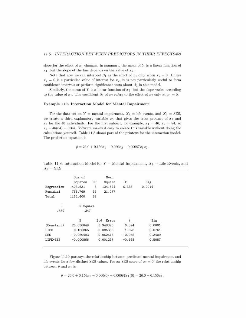
Example 11.6 Interaction Model for Mental Impairment
For the data set on Y = mental impairment, X1 = life events, and X2 = SES,
we create a third explanatory variable x3 that gives the cross product of x1 and
x2 for the 40 individuals. For the first subject, for example, x1 = 46, x2 = 84, so
x3 = 46(84) = 3864. Software makes it easy to create this variable without doing the
calculations yourself. Table 11.8 shows part of the printout for the interaction model.
The prediction equation is
y = 26.0 + 0.156x1 − 0.060x2 − 0.00087x1x2.
Table 11.8: Interaction Model for Y = Mental Impairment, X1 = Life Events, andX2 = SES
Sum of Mean
Squares DF Square F Sig
Regression 403.631 3 134.544 6.383 0.0014
Residual 758.769 36 21.077
Total 1162.400 39
R R Square
.589 .347
B Std. Error t Sig
(Constant) 26.036649 3.948826 6.594 0.0001
LIFE 0.155865 0.085338 1.826 0.0761
SES -0.060493 0.062675 -0.965 0.3409
LIFE*SES -0.000866 0.001297 -0.668 0.5087
Figure 11.10 portrays the relationship between predicted mental impairment and
life events for a few distinct SES values. For an SES score of x2 = 0, the relationship
The reduced model without the interaction terms is
E(Y ) = α + β1x1 + β2x2 + β3x3.
The test comparing the complete model to the reduced model has H0: β4 = β5 =
β6 = 0.
11.6. COMPARING REGRESSION MODELS 463
Comparing Models by Comparing SSE or R2 Values
The test statistic for comparing two regression models compares the residual sums
of squares for the two models. Denote SSE =∑
(y − y)2 for the reduced model by
SSEr and for the complete model by SSEc. Now, SSEr ≥ SSEc, because the reduced
model has fewer predictors and tends to make poorer predictions. Even if H0 were
true, we would not expect the estimates of the extra parameters and the difference
(SSEr−SSEc) to equal 0. Some reduction in error occurs from fitting the extra terms
because of sampling variability.
The test statistic uses the reduction in error, SSEr − SSEc, that results from
adding the extra variables. It has df = the number of extra terms in the complete
model. An equivalent statistic uses the R2 values, R2c for the complete model and R2
r
for the reduced model. The test statistic equals
F =(SSEr − SSEc)/df1
SSEc/df2=
(R2c − R2
r)/df1
(1 − R2c)/df2
,
where df1 is the number of extra terms in the complete model and df2 is the usual
residual df for the complete model, which is df2 = n − (k + 1). A relatively large
reduction in error (or relatively large increase in R2) yields a large F test statistic
and small P -value. As usual for F statistics, the P -value is the right-tail probability.
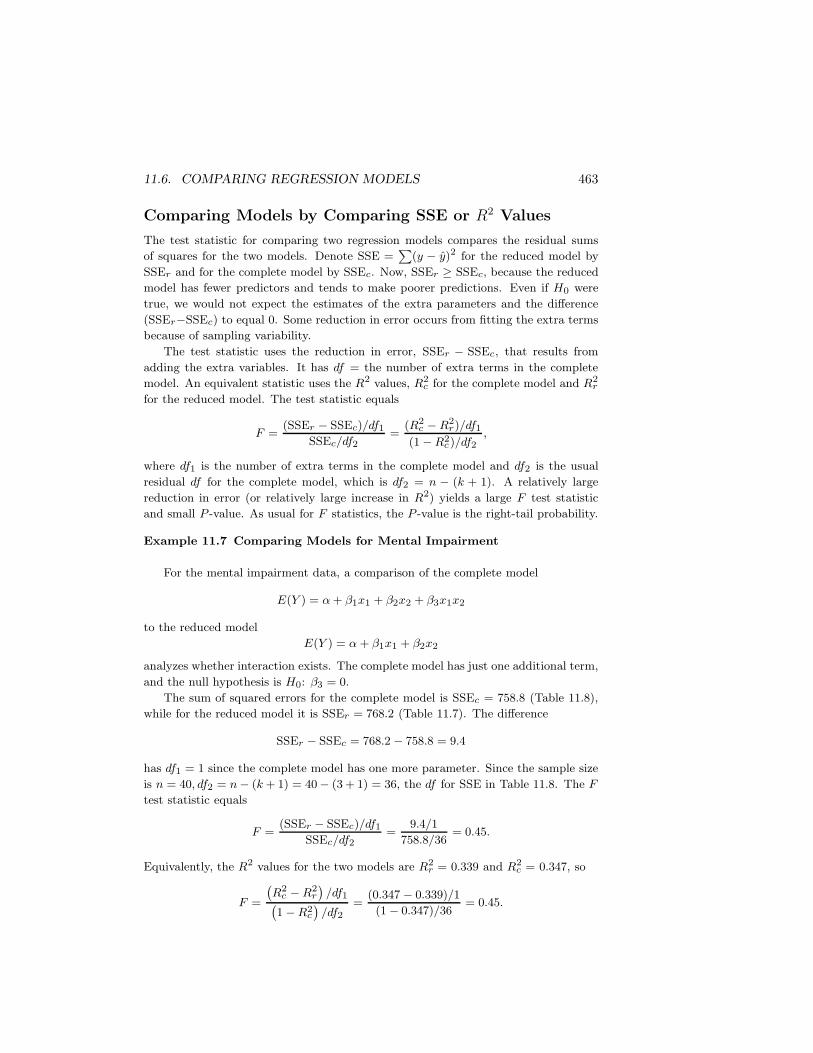
Example 11.7 Comparing Models for Mental Impairment
For the mental impairment data, a comparison of the complete model
E(Y ) = α + β1x1 + β2x2 + β3x1x2
to the reduced model
E(Y ) = α + β1x1 + β2x2
analyzes whether interaction exists. The complete model has just one additional term,
and the null hypothesis is H0: β3 = 0.
The sum of squared errors for the complete model is SSEc = 758.8 (Table 11.8),
while for the reduced model it is SSEr = 768.2 (Table 11.7). The difference
SSEr − SSEc = 768.2 − 758.8 = 9.4
has df1 = 1 since the complete model has one more parameter. Since the sample size
is n = 40, df2 = n − (k + 1) = 40 − (3 + 1) = 36, the df for SSE in Table 11.8. The F
test statistic equals
F =(SSEr − SSEc)/df1
SSEc/df2=
9.4/1
758.8/36= 0.45.
Equivalently, the R2 values for the two models are R2r = 0.339 and R2
c = 0.347, so
F =
(
R2c − R2
r
)
/df1(
1 − R2c
)
/df2
=(0.347 − 0.339)/1
(1 − 0.347)/36= 0.45.
464 CHAPTER 11. MULTIPLE REGRESSION AND CORRELATION
From software, the P -value from the F distribution with df1 = 1 and df2 = 36 is
P = 0.51. There is little evidence that the complete model is better. The null
hypothesis seems plausible, so the reduced model is adequate.
When H0 contains a single parameter, the t test is available. In fact, from the
previous section (and Table 11.8), the t statistic equals
t =b3se
=−0.00087
0.0013= −0.67.
It also has a P -value of 0.51 for Ha: β3 6= 0. We get the same result with the t test as
with the F test for complete and reduced models. In fact, the F test statistic equals
the square of the t statistic. (Refer to the final subsection in Section 11.4.)
2
The t test method is limited to testing one parameter at a time. The F test can
test several regression parameters together to analyze whether at least one of them is
nonzero, such as in the global F test of H0 : β1 = · · · = βk = 0 or the test comparing
a complete model to a reduced model. F tests are equivalent to t tests only when H0
contains a single parameter.
11.7 Partial Correlation∗
Multiple regression models describe the effect of an explanatory variable on the re-
sponse variable while controlling for other variables of interest. Related measures
describe the strength of the association. For example, to describe the association
between mental impairment and life events, controlling for SES, we could ask, “Con-
trolling for SES, what proportion of the variation in mental impairment does life
events explain?”
These measures describe the partial association between Y and a particular pre-
dictor, whereas the multiple correlation and R2 describe the association between Y
and the entire set of predictors in the model. The partial correlation is based on the
ordinary correlations between each pair of variables. For a single control variable, it
is defined as follows:
Partial Correlation
The sample partial correlation between Y and X2, controlling for X1, is
rY X2·X1=
rY X2− rY X1
rX1X2√
(
1 − r2Y X1
) (
1 − r2X1X2
)
.
In the symbol rY X2·X1, the variable to the right of the dot represents the controlled
variable. The analogous formula for rY X1·X2(i.e., controlling X2) is
rY X1·X2=
rY X1− rY X2
rX1X2√
(
1 − r2Y X2
) (
1 − r2X1X2
)
.
11.7. PARTIAL CORRELATION∗ 465
Since one variable is controlled, the partial correlations rY X1·X2and rY X2·X1
are
called first-order partial correlations.
Example 11.8 Partial Correlation Between Education and Crime Rate
Example 11.1 discussed a data set for counties in Florida, with Y = crime rate,
X1 = education, and X2 = urbanization. The pairwise correlations are rY X1=
0.468, rY X2= 0.678, and rX1X2
= 0.791. It was surprising to observe a positive
correlation between crime rate and education. Can it be explained by their joint
dependence on urbanization? This is plausible if the association disappears when we
control for urbanization.
The partial correlation between crime rate and education, controlling for urban-
ization, equals
rY X1·X2=
rY X1− rY X2
rX1X2√
(1 − r2Y X2
)(1 − r2X1X2
)=
0.468 − 0.678(0.791)√
(1 − 0.6782) (1 − 0.7912)= −0.152.
Not surprisingly, rY X1·X2is much smaller than rY X1
. It even has a different direction,
illustrating Simpson’s paradox. The relationship between crime rate and education
may well be spurious, reflecting their joint dependence on urbanization.
2
Interpreting Partial Correlations
The partial correlation has properties similar to those for the ordinary correlation
between two variables, such as a range of −1 to +1, larger absolute values representing
stronger associations, and value free of the units. We list the properties below for
rY X1·X2, but analogous properties apply to rY X2·X1
.
• rY X1·X2falls between −1 and +1.
• The larger the absolute value of rY X1·X2, the stronger the association between
Y and X1, controlling for X2.
• The value of a partial correlation does not depend on the units of measurement
of the variables.
• rY X1·X2has the same sign as the partial slope (b1) for the effect of x1 in the
prediction equation y = a+b1x1+b2x2. This happens because the same variable
(x2) is controlled in the model as in the correlation.
• Under the assumptions for conducting inference for multiple regression (see
the beginning of Section 11.4), rY X1·X2estimates the correlation between Y
and X1 at every fixed value of X2. If we could control X2 by considering
a subpopulation of subjects all having the same value on X2, then rY X1·X2
estimates the correlation between Y and X1 for that subpopulation.
466 CHAPTER 11. MULTIPLE REGRESSION AND CORRELATION
• The sample partial correlation is identical to the correlation computed for the
points in the partial regression plot (Section 11.2).
Interpreting Squared Partial Correlations
Like r2 and R2, the square of a partial correlation has a proportional reduction in
error (PRE) interpretation. It states that r2Y X2·X1
is the proportion of variation in
Y explained by X2, controlling for X1. This squared measure describes the effect of
removing from consideration the portion of the total sum of squares (TSS) in Y that
is explained by X1, and then finding the proportion of the remaining unexplained
variation in Y that is explained by X2.
Squared Partial Correlation
The square of the partial correlation rY X2·X1represents the proportion of the variation
in Y that is explained by X2, out of that left unexplained by X1. It equals
r2Y X2·X1
=R2 − r2
Y X1
1 − r2Y X1
=Partial proportion explained uniquely by X2
Proportion unexplained by X1.
Recall from Section 9.4 that r2Y X1
represents the proportion of the variation in
Y explained by X1. The remaining proportion (1 − r2Y X1
) represents the variation
left unexplained. When X2 is added to the model, it accounts for some additional
variation. The total proportion of the variation in Y accounted for by X1 and X2
jointly is R2 for the model with both X1 and X2 as explanatory variables. So, R2 −r2Y X1
is the additional proportion of the variability in Y explained by X2, after the
effects of X1 have been removed or controlled. The maximum this difference could
be is 1 − r2Y X1
, the proportion of variation yet to be explained after accounting for
the influence of X1. The additional explained variation R2 − r2Y X1
divided by this
maximum possible difference is a measure that has a maximum possible value of 1. In
fact, as the above formula suggests, this ratio equals the squared partial correlation
between Y and X2, controlling for X1.
Figure 11.11 illustrates this property of the squared partial correlation. It shows
the ratio of the partial contribution of X2 beyond that of X1, namely, R2 − r2Y X1
,
divided by the proportion (1 − r2Y X1
) left unexplained by X1. Similarly, the square
of rY X1·X2equals
r2Y X1·X2
=R2 − r2
Y X2
1 − r2Y X2
,
the proportion of variation in Y explained by X1, out of that part unexplained by X2.
Example 11.9 Partial Correlation of Life Events with Mental Impairment
We return to the mental health study, with Y = mental impairment, X1 = life
events, X2 = SES. Software reports the correlation matrix,
11.7. PARTIAL CORRELATION∗ 467
IMPAIR LIFE SES
IMPAIR 1.000 .372 -.399
LIFE .372 1.000 .123
SES -.399 .123 1.000
So, rY X1= 0.372, rY X2
= −0.399, and rX1X2= 0.123. By its definition, the partial
correlation between mental impairment and life events, controlling for SES, is
rY X1·X2=
rY X1− rY X2
rX1X2√
(
1 − r2Y X2
) (
1 − r2X1X2
)
=0.372 − (−0.399)(0.123)
√
[1 − (−0.399)2] (1 − 0.1232)= 0.463.
The partial correlation, like the correlation of 0.37 between mental impairment and
life events, is moderately positive.
Since r2Y X1·X2
= (0.463)2 = 0.21, controlling for SES, 21% of the variation in
mental impairment is explained by life events. Alternatively, since R2 = 0.339 (Table
11.7),
r2Y X1·X2
=R2 − r2
Y X2
1 − r2Y X2
=0.339 − (−0.399)2
1 − (−0.399)2= 0.21.
2
Higher-Order Partial Correlations
One reason we showed the connection between squared partial correlation values and
R-squared is that this approach also works when the number of control variables
exceeds one. For example, with three predictors, let R2Y (X1,X2,X3) denote the value
of R2. The square of the partial correlation between Y and X3, controlling for X1 and
X2, relates to how much larger this is than the R2 value for the model with only X1
and X2 as predictors, which we denote by R2Y (X1,X2). The squared partial correlation
is
r2Y X3·X1,X2
=R2
Y (X1,X2,X3) − R2Y (X1,X2)
1 − R2Y (X1,X2)
.
In this expression, R2Y (X1,X2,X3) −R2
Y (X1,X2)is the increase in the proportion of
explained variance from adding x3 to the model. The denominator 1 − R2Y (X1,X2)
is
the proportion of the variation left unexplained when x1 and x2 are the only predictors
in the model.
The partial correlation rY X3·X1,X2is called a second-order partial corre-
lation , since it controls two variables. It has the same sign as b3 in the prediction
equation y = a + b1x1 + b2x2 + b3x3, which also controls x1 and x2 in describing the
effect of x1.
Inference for Partial Correlations
Controlling for a certain set of variables, the slope of the partial effect of a predictor is 0
in the same situations in which the partial correlation between Y and that predictor is
0. An alternative formula for the t test for a partial effect uses the partial correlation.
468 CHAPTER 11. MULTIPLE REGRESSION AND CORRELATION
With k predictors in the model, the equivalent t test statistic is
t =partial correlation
√
(1 − squared partial correlation)/[n − (k + 1)].
This statistic has the t distribution with df = n − (k + 1). It equals the t statistic
based on the partial slope estimate and, hence, has the same P -value.
We illustrate by testing that the population partial correlation between mental
impairment and life events, controlling for SES, is 0. From Example 11.9, rY X1·X2=
0.463. There are k = 2 explanatory variables and n = 40 observations. The test
statistic equals
t =rY X1·X2
√
(1 − r2Y X1·X2
)/[n − (k + 1)]=
0.463√
[1 − (0.463)2]/37= 3.18.
This equals the test statistic for H0: β1 = 0 in Table 11.5. Thus, the P -value is also
the same, P = 0.003.
When no variables are controlled (i.e., the number of explanatory variables is
k = 1), the t statistic formula simplifies to
t =r
√
(1 − r2)/(n − 2).
This is the statistic for testing that the population bivariate correlation equals 0
(Section 9.5). Confidence intervals for partial correlations are more complex. They
require a log transformation such as shown for the correlation in Exercise 65 in Chapter
9.
11.8 Standardized Regression Coefficients∗
As in bivariate regression (Recall Section 9.4), the sizes of regression coefficients in
multiple regression models depend on the units of measurement for the variables. To
compare the relative effects of two explanatory variables, it is appropriate to compare
their coefficients only if the variables have the same units. Otherwise, standardized
versions of the regression coefficients provide more meaningful comparisons.
Standardized Regression Coefficient
The standardized regression coefficient for an explanatory variable represents the
change in the mean of Y , in Y standard deviations, for a one standard deviation increase
in that variable, controlling for the other explanatory variables in the model. We denote
them by β∗
1 , β∗
2 , . . . .
If |β∗
2 | > |β∗
1 |, for example, then a standard deviation increase in X2 has a greater
partial effect on Y than does a standard deviation increase in X1.
11.8. STANDARDIZED REGRESSION COEFFICIENTS∗ 469
The Standardization Mechanism
The standardized regression coefficients represent the values the regression coefficients
take when the units are such that Y and the explanatory variables all have equal
standard deviations. We standardize the partial regression coefficients by adjusting for
the differing standard deviation of Y and each Xi. Let sy denote the sample standard
deviation of Y , and let sx1, sx2
, . . . , sxkdenote the sample standard deviations of the
explanatory variables.
The estimates of the standardized regression coefficients are
b∗1 = b1
(
sx1
sy
)
, b∗2 = b2
(
sx2
sy
)
, . . . .
Example 11.10 Standardized Coefficients for Mental Impairment
The prediction equation relating mental impairment to life events and SES is
y = 28.23 + 0.103x1 − 0.097x2.
Table 11.2 reported the sample standard deviations sy = 5.5, sx1= 22.6, and sx2
=
25.3. Since the unstandardized coefficient of x1 is b1 = 0.103, the estimated standard-
ized coefficient is
b∗1 = b1
(
sx1
sy
)
= 0.103(
22.6
5.5
)
= 0.43.
Since b2 = −0.097, the standardized value equals
b∗2 = b2
(
sx2
sy
)
= −0.097(
25.3
5.5
)
= −0.45.
The estimated change in the mean of Y for a standard deviation increase in x1,
controlling for x2, has similar magnitude as the estimated change for a standard
deviation increase in x2, controlling for x1. However the partial effect of x1 is positive,
whereas the partial effect of x2 is negative.
Table 11.9, which repeats Table 11.5, shows how SPSS reports the estimated stan-
dardized regression coefficients. It uses the heading BETA, reflecting the alternative
name beta weights for these coefficients.
2
470 CHAPTER 11. MULTIPLE REGRESSION AND CORRELATION
Table 11.9: SPSS Printout for Fit of Multiple Regression Model to Mental Impair-ment Data
Unstandardized Standardized
Coefficients Coefficients
B Std. Error Beta t Sig.
(Constant) 28.230 2.174 12.984 .000
LIFE .103 .032 .428 3.177 .003
SES -.097 .029 -.451 -3.351 .002
Properties of Standardized Regression Coefficients
For bivariate regression, standardizing the regression coefficient yields the correla-
tion. For the multiple regression model, the standardized partial regression coefficient
relates to the partial correlation (Exercise 67), and it usually takes similar value.
Unlike the partial correlation, however, b∗i need not fall between −1 and +1. A
value |b∗i | > 1 occasionally occurs when Xi is highly correlated with the set of other
explanatory variables in the model. In such cases, the standard errors are usually
large and the estimates are unreliable.
Since a standardized regression coefficient is a multiple of the unstandardized
coefficient, one equals 0 when the other does. The test of H0: β∗
i = 0 is equivalent to
the t test of H0: βi = 0. It is unnecessary to have separate tests for these coefficients.
In the sample, the magnitudes of the {b∗i } have the same relative sizes as the t statistics
from those tests. For example, the predictor with the greatest standardized partial
effect is the one that has the largest t statistic, in absolute value.
Standardized Form of Prediction Equation∗
Regression equations have an expression using the standardized regression coefficients.
In this equation, the variables appear in standardized form.
Notation for Standardized Variables
Let zY , zX1, . . . , zXk
denote the standardized versions of the variables Y, X1, . . . , Xk .
For instance, zY = (y − y)/sy represents the number of standard deviations that an
observation on y falls from its mean.
Each subject’s scores on y, x1, . . . , xk have corresponding z-scores for zY , zX1, . . . , zXk
.
If a subject’s score on x1 is such that zX1= (x1 − x1)/sx1
= 2.0, for instance, then
that subject falls two standard deviations above the mean x1 on that variable.
Let zY = (y − y)/sy denote the predicted z-score for the response variable. For
the standardized variables and the estimated standardized regression coefficients, the
prediction equation is
zY = b∗1zX1+ b∗2zX2
+ · · · + b∗kzXk.
11.8. STANDARDIZED REGRESSION COEFFICIENTS∗ 471
This equation predicts how far an observation on y falls from its mean, in standard
deviation units, based on how far the explanatory variables fall from their means, in
standard deviation units. The standardized coefficients are the weights attached to
the standardized explanatory variables in contributing to the predicted standardized
response variable.
Example 11.11 Standardized Prediction Equation for Mental Impairment
Example 11.10 found that the estimated standardized regression coefficients for
the life events and SES predictors of mental impairment are b∗1 = 0.43 and b∗2 = −0.45.
The prediction equation relating the standardized variables is therefore
zY = 0.43zX1− 0.45zX2
.
Consider a subject who is two standard deviations above the mean on life events
but two standard deviations below the mean on SES. This subject has a predicted
standardized mental impairment of
zY = 0.43(2) − 0.45(−2) = 1.8.
The predicted mental impairment for that subject is 1.8 standard deviations above
the mean. If the distribution of mental impairment is approximately normal, this
subject might well have mental health problems, since only about 4% of the scores in
a normal distribution fall at least 1.8 standard deviations above their mean.
2
In the prediction equation with standardized variables, no intercept term appears.
Why is this? When the standardized explanatory variables all equal 0, those variables
all fall at their means. Then, y = y, so that
zY =y − y
sy= 0.
So, this merely tells us that a subject who falls at the mean on each explanatory
variable is predicted to fall at the mean on the response variable.
Cautions in Comparing Standardized Regression Coeffi-
cients
To assess which predictor in a multiple regression model has the greatest impact on the
response variable, it is tempting to compare their standardized regression coefficients.
Make such comparisons with caution. In some cases, the observed differences in the
b∗i may simply reflect sampling error. In particular, when multicollinearity exists, the
standard errors are high and the estimated standardized coefficients may be unstable.
Keep in mind also that the effects are partial ones, depending on which other
variables are in the model. An explanatory variable that seems important in one
472 CHAPTER 11. MULTIPLE REGRESSION AND CORRELATION
system of variables may seem unimportant when other variables are controlled. For
example, it is possible that |b∗2| > |b∗1| in a model with two explanatory variables, yet
when a third explanatory variable is added to the model, |b∗2| < |b∗1|.It is unnecessary to standardize to compare the effect of the same variable for two
groups, such as in comparing the results of separate regressions for females and males,
since the units of measurement are the same in each group. In fact, it is usually unwise
to standardize in this case, because the standardized coefficients are more susceptible
than the unstandardized coefficients to differences in the standard deviations of the
predictors. For instance, Section 9.6 showed that the correlation depends strongly on
the range of x-values sampled. Two groups that have the same value for an estimated
regression coefficient have different standardized coefficients if the standard deviation
of the predictor differs for the two groups.
Finally, if an explanatory variable is highly correlated with the set of other ex-
planatory variables, it is artificial to conceive of that variable changing while the
others remain fixed in value. As an extreme example, suppose Y = height, X1 =
length of left leg, and X2 = length of right leg. The correlation between X1 and X2
is extremely close to 1. It does not make much sense to imagine how Y changes as
X1 changes while X2 is controlled.
11.9 Chapter Summary
This chapter generalized the bivariate regression model to include additional explana-
tory variables. The multiple regression equation relating a response variable Y
to a set of k explanatory variables is
E(Y ) = α + β1x1 + β2x2 + · · · + βkxk.
• The {βi} are partial regression coefficients . The value βi is the change
in the mean of Y for a one-unit change in xi, controlling for the other variables
in the model.
• The multiple correlation R describes the association between Y and the
collective set of explanatory variables. It equals the correlation between the
observed and predicted y-values. It falls between 0 and 1.
• R2 = (TSS − SSE)/TSS represents the proportional reduction in error from
predicting Y using the prediction equation y = a + b1x1 + b2x2 + · · · + bkxk
instead of y. It equals the square of the multiple correlation.
• A partial correlation , such as rY X1·X2, describes the association between
two variables, controlling for others. It falls between −1 and +1.
• The squared partial correlation between Y and xi represents the proportion of
the variation in Y that can be explained by xi, out of that part left unexplained
by a set of control variables.
Chap. 11 Problems 473
• An F statistic tests H0 : β1 = β2 = · · · = βk = 0, that the response variable
is independent of all the predictors. A small P -value suggests that at least one
predictor affects the response.
• Individual t tests and confidence intervals for {βi} analyze partial effects of each
predictor, controlling for the other variables in the model.
• Interaction between x1 and x2 in their effects on Y means that the effect of
either predictor changes as the value of the other predictor changes. We can
allow this by introducing cross-products of explanatory variables to the model,
such as the term β3(x1x2).
• To compare regression models, a complete model and a simpler reduced
model, the F test compares the SSE values or R2 values.
• Standardized regression coefficients do not depend on the units of mea-
surement. The estimated standardized coefficient b∗i describes the change in Y ,
in Y standard deviation units, for a one standard deviation increase in xi, con-
trolling for the other explanatory variables.
To illustrate, with k = 2 explanatory variables, the prediction equation is
Y = a + b1x1 + b2x2.
Fixing x2, a straight line describes the relation between Y and x1. Its slope b1is the change in y for a one-unit increase in x1, controlling for x2. The multiple
correlation R is at least as large as the correlations between Y and each predictor.
The squared partial correlation r2Y X2·X1
is the proportion of the variation of Y that
is explained by x2, out of that part of the variation left unexplained by x1. The
estimated standardized regression coefficient b∗1 = b1(sx1/sy) describes the effect of a
standard deviation change in x1, controlling for x2.
Table 11.10 summarizes the basic properties and inference methods for these mea-
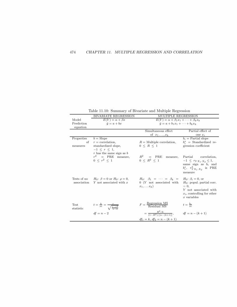
sures and those introduced in Chapter 9 for bivariate regression.
The model studied in this chapter is still somewhat restrictive in the sense that
all the predictors are quantitative. The next chapter shows how to include categorical
predictors in the model.
PROBLEMS
Practicing the Basics
1. For students at Walden University, the relationship between Y = college GPA
(with range 0–4.0) and X1 = high school GPA (range 0–4.0) and X2 = college
d) Can be used to test whether the model E(Y ) = α + β1x1 + β2x2 gives a
significantly better fit than the model E(Y ) = α + β1x1 + β2x3.
55. Explain the difference in the purposes of the correlation, the multiple correla-
tion, and the partial correlation.
56. Let Y = height, X1 = length of right leg, X2 = length of left leg. Describe
what you expect for the relative sizes of the three pairwise correlations, R, and
rY X2·X1.
57. Give an example of three variables for which you expect β 6= 0 in the model
E(Y ) = α + βx1 but β1 = 0 in the model E(Y ) = α + β1x1 + β2x2.
58. For the models E(Y ) = α + βx and E(Y ) = α + β1x1 + β2x2, express null
hypotheses in terms of correlations that are equivalent to the following:
a) H0: β = 0
b) H0: β1 = β2 = 0
c) H0: β2 = 0
59. * Whenever X1 and X2 are uncorrelated, then R2 for the model E(Y ) = α +
β1x1 + β2x2 satisfies R2 = r2Y X1
+ r2Y X2
. In this case, draw a figure that
portrays the variability in Y , the part of that variability explained by each of
X1 and X2, and the total variability explained by both of them together.
60. * Which of the following sets of correlations would you expect to yield the
highest R2 value? Why?
a) rY X1= 0.4, rY X2
= 0.4, rX1X2= 0.0
b) rY X1= 0.4, rY X2
= 0.4, rX1X2= 0.5
c) rY X1= 0.4, rY X2
= 0.4, rX1X2= 1.0
492 CHAPTER 11. MULTIPLE REGRESSION AND CORRELATION
61. * Suppose the correlation between Y and X1 equals the multiple correlation
between Y and X1 and X2. What does this imply about the partial correlation
rY X2·X1? Interpret.
62. * Software reports four types of sums of squares in multiple regression models.
The Type I (sometimes called sequential) sum of squares represents the vari-
ability explained by a variable, controlling for variables previously entered into
the model. The Type III (sometimes called partial) sum of squares represents
the variability explained by that variable, controlling for all other variables in
the model.
a) For any multiple regression model, explain why the Type I sum of squares
for x1 is the regression sum of squares for the bivariate model with x1 as the
predictor, whereas the Type I sum of squares for x2 equals the amount by which
SSE decreases when x2 is added to the model.
b) Explain why the Type I sum of squares for the last variable entered into a
model is the same as the Type III sum of squares for that variable.
63. * The sample value of R2 tends to overestimate the population value, because
the sample data fall closer to the sample prediction equation than to the true
population regression equation. This bias is greater if n is small or the number
of predictors k is large. A somewhat better estimate is adjusted R2,
R2adj = 1 − s2
s2y
= R2 −[
k
n − (k + 1)
]
(1 − R2),
where s2 is the estimated conditional variance (i.e., the mean square error) and
s2Y is the sample variance of Y .
a) Suppose R2 = 0.339 for a model with k = 2 explanatory variables (such as
in Table 11.5). Find R2adj for the following sample sizes: 10, 40 (as in the text
example), 100, and 1000. Show that R2adj approaches R2 in value as n increases.
b) Show that R2adj is negative when R2 < k/(n − 1). This is undesireable, and
R2adj is equated to 0 in such cases. (Also, unlike R2, R2
adj could decrease when
we add an explanatory variable to a model.)
64. * Let R2Y (X1,...Xk) denote R2 for the multiple regression model with k explana-
tory variables. Explain why
rY Xk·X1,...,Xk−1=
R2Y (X1,...,Xk) − R2
Y (X1,...,Xk−1)
1 − RY (X1,...,Xk−1).
65. * The numerator R2 − r2Y X1
of the squared partial correlation r2Y X2·X1
gives
the increase in the proportion of explained variation from adding X2 to the
model. This increment, denoted by r2Y (X2·X1)
, is called the squared semipar-
tial correlation. One can use squared semipartial correlations to partition the
Chap. 11 Problems 493
variation in the response variable. For instance, for three explanatory variables,
R2Y (X1,X2,X3) = r2
Y X1+ (R2
Y (X1,X2) − r2Y X1
) + (R2Y (X1,X2,X3) − R2
Y (X1,X2))
= r2Y X1
+ r2Y (X2·X1) + r2
Y (X3·X1,X2).
The total variation in Y explained by X1, X2, and X3 together partitions into:
(i) the proportion explained by X1 (i.e., r2Y X1
), (ii) the proportion explained
by X2 beyond that explained by X1 (i.e., r2Y (X2·X1)), and (iii) the proportion
explained by X3 beyond that explained by X1 and X2 (i.e, r2Y (X3·X1,X2)).
These correlations have the same ordering as the t statistics for testing partial
effects, and some researchers use them as indices of importance of the predictors.
a) In Example 11.2 on mental impairment, show that r2Y (X2·X1)
= 0.20 and
r2Y (X1·X2) = 0.18. Interpret.
b) Explain why the squared semipartial correlation r2Y (X2·X1) cannot be larger
than the squared partial correlation r2Y X2·X1
.
66. * The least squares prediction equation provides predicted values Y with the
strongest possible correlation with Y , out of all possible prediction equations
of that form. That is, the least squares equation yields the best prediction
of Y in the sense that it represents the linear reduction of X1, . . . , Xk to the
single variable that is most strongly correlated with Y . Based on this property,
explain why the multiple correlation cannot decrease when one adds a variable
to a multiple regression model. (Hint: The prediction equation for the simpler
model is a special case of a prediction equation for the full model that has
coefficient 0 for the added variable.)
67. * Let b∗i denote the estimated standardized regression coefficient when Xi is
treated as the response variable and Y as an explanatory variable, controlling
for the same set of other variables. Then, b∗i need not equal b∗i . The partial
correlation between Y and Xi, which is symmetric in the order of the two
variables, satisfies
r2Y Xi·— = b∗i b∗i .
a) From this formula, explain why the partial correlation must fall between b∗iand b∗i . (Note: When a =
√bc, a is said to be the geometric average of b and
c.)
b) Even though b∗i does not necessarily fall between −1 and +1, explain why
b∗i b∗i cannot exceed 1.
68. * Chapters 12 and 13 show how to incorporate categorical predictors in regres-
sion models, and this exercise provides a preview. Table 11.21 shows part of a
printout for a model for the “house selling price 2” data set at the text website,
with Y = selling price of home, X1 = size of home, and X2 = whether the
house is new (1 = yes, 0 = no).
a) Report the prediction equation. By setting x2 = 0 and then 1, construct the
494 CHAPTER 11. MULTIPLE REGRESSION AND CORRELATION
two separate lines for older and for new homes. Note that the model implies
that the slope effect of size on selling price is the same for each.
b) Since x2 takes only the values 0 and 1, explain why the coefficient of x2
estimates the difference of mean selling prices between new and older homes,
controlling for house size.
Table 11.23:
B Std. Error t Sig
(Constant) -26.089 5.977 -4.365 0.0001
SIZE 72.575 3.508 20.690 0.0001
NEW 19.587 3.995 4.903 0.0001
69. * Refer to the previous exercise. When we add an interaction term, we get
y = −16.6 + 66.6x1 − 31.8x2 + 29.4(x1x2).
a) Interpret the fit by reporting the prediction equation between selling price
and size of house separately for new homes (x2 = 1) and for old homes (x2 =
0). Interpret. (This fit is equivalent to fitting lines separately to the data for
new homes and for old homes.)
b) Interpret the fit by reporting the difference between the predicted selling
prices for new and old homes for houses with x1 equal to (i) 1.5, (ii) 2.0, (iii)
2.5.
c) A plot of the data shows an outlier, a new home with a very high selling
price. When that observation is removed from the data set and the model is
re-fitted, y = −16.6 + 66.6x1 + 9.0x2 + 5.0(x1x2). Re-do (a), and explain how
an outlier can have a large impact on a regression analysis.
11.9.1 Bibliography
DeMaris, A. (2004). Regression with Social Data: Modeling Continuous and Limited
Response Variables. Wiley.
Draper, N. R. and Smith, H. (1998). Applied Regression Analysis, 3rd ed., Wiley.
Holzer, C. E., III (1977). The Impact of Life Events on Psychiatric Symptomatology.
Ph.D. dissertation, University of Florida, Gainesville.
Kutner, M. H., Nachtsheim, C. J., and Neter, J. (2004). Applied Linear Regression
Models, 4th ed. McGraw-Hill/Irwin.
Weisberg, S. (2005). Applied Linear Regression, 3rd ed., Wiley.
Chap. 11 Problems 495
Figure 11.5: A Scatterplot Matrix: Scatterplots for Pairs of Variables fromTable 11.1
((Fig. 11.5 from 3e))
Figure 11.6: Partial Regression Plot for Mental Impairment and Life Events,Controlling for SES. This plots the residuals from regressing mental impairmenton SES against the residuals from regressing life events on SES.
((Include new Fig. 11.6))
Figure 11.7: Partial Regression Plot for Mental Impairment and SES, Control-ling for Life Events. This plots the residuals from regressing mental impairmenton life events against the residuals from regressing SES on life events.
((Include new Fig. 11.7))
Figure 11.8: R2 Does Not Increase Much When x3 Is Added to the Model
Already Containing x1 and x2
((Fig. 11.8 in 3e))
Figure 11.9: The F Distribution and the P -Value for F Tests. Larger F valuesgive stronger evidence against H0.
((Fig. 11.9 in 3e))
Figure 11.10: Portrayal of Interaction between x1 and x2 in their Effects on Y .
((Fig. 11.10 in 3e; if possible, change to lower-case letters))
496 CHAPTER 11. MULTIPLE REGRESSION AND CORRELATION
Figure 11.11: Representation of r2Y X2·X1
as the Proportion of Variability ThatCan Be Explained by X2, of that Left Unexplained by X1