38
Chapter 3 Linear Programming: Computer Solution and Sensitivity Analysis BIT 2406 1
| Date post: | 25-Dec-2015 |
| Category: |
Documents |
| Upload: | parth-patel |
| View: | 213 times |
| Download: | 1 times |

Chapter 3Linear Programming: Computer Solution and Sensitivity Analysis
BIT 2406 1

Chapter Topics
• Computer Solution
• Sensitivity Analysis
BIT 2406 2

Simplex Method
• The Simplex method is a procedure involving a set of mathematical steps to solve linear programming problems.
• Software for computer solution of linear programming problems is based on the Simplex method.
• Tutorial on the Simplex method is included in the online material.
• An online tutorial demonstrating the Simplex method, is available here: http://people.hofstra.edu/Stefan_waner/RealWorld/tutorialsf4/frames4_3.html
• In this course, we will use Excel Solver to look at computerized solution of linear programming problems.
BIT 2406 3

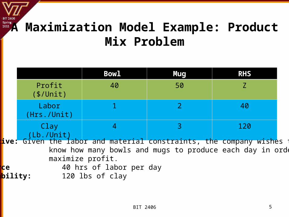
A Maximization Model Example: Product Mix Problem
BIT 2406 4
A Maximization Model Example: Product Mix Problem
Bowl Mug RHS
Profit ($/Unit) 40 50 Z
Labor (Hrs./Unit) 1 2 40
Clay (Lb./Unit) 4 3 120
BIT 2406 5
Objective: Given the labor and material constraints, the company wishes to know how many bowls and mugs to produce each day in order to maximize profit.Resource 40 hrs of labor per dayAvailability: 120 lbs of clay

A Maximization Model Example: Product Mix Problem
• Decision x1 = number of bowls to produce per day Variables: x2 = number of mugs to produce per day
• Objective maximize Z = 40x1 + 50x2
Function:
• Resource 1x1 + 2x2 40 hours of labor Constraints: 4x1 + 3x2 120 pounds of clay
• Non-Negativity x1 0; x2 0 Constraints*:
BIT 2406 6
*Non-negativity constraints: restrict the decision variables to zero or positive values.

Spreadsheet Setup
BIT 2406 7

Formula View
BIT 2406 8

Calling and Setting Up Solver
BIT 2406 9
5
0
1
2
34

Solver Options
BIT 2406 10

Solver Results
BIT 2406 11

Answer Report
BIT 2406 12

Sensitivity Analysis
• Sensitivity analysis is the analysis of the effect of parameter changes on the optimal solution.
• Changes may be reactions to anticipated uncertainties in the parameters or to new or changed information concerning the model.
• The obvious solution is to change the model parameter, solve the model again and compare the results.
• However, in some cases the effect of changes on the model can be determined without solving the problem again.
BIT 2406 13

Optimal Solution with Original ModelOptimal Solution with Original Model
0,
clay of lb.12034
labor of hr.402
subject to
5040 maximize
produced mugs ofnumber
produced bowls ofnumber
21
21
21
21
2
1
xx
xx
xx
xxZ
x
x
BIT 2406 14

Impact of Changing Objective Function Parameter (Coefficient of x1)
0,
clay of lb.12034
labor of hr.402
subject to
50100$ maximize
produced mugs ofnumber
produced bowls ofnumber
21
21
21
21
2
1
xx
xx
xx
xxZ
x
x
BIT 2406 15

Impact of Changing Objective Function Parameter (Coefficient of x2)
0,
clay of lb.12034
labor of hr.402
subject to
10040$ maximize
produced mugs ofnumber
produced bowls ofnumber
21
21
21
21
2
1
xx
xx
xx
xxZ
x
x
BIT 2406 16

Sensitivity Range for an Objective Function Coefficient
• The sensitivity range for an objective coefficient is the range of values over which the current optimal solution point will remain optimal.
• The sensitivity range for the xi coefficient is designated as ci.
BIT 2406 17

Sensitivity Range for an Objective Function Coefficient (x1)
BIT 2406 18

Sensitivity Range for an Objective Function Coefficient (x2)
BIT 2406 19

• The complete sensitivity range for the x1 coefficient is: 25 ≤ c1 ≤ 66.67.
• This means that the profit for a bowl can vary anywhere between $25.00 and $66.67, and the optimal solution point, x1 = 24 and x2 = 8 will not change.
• The total profit, however, will change depending on what c1 actually is.
• In this case, a manager would know how much profit can be altered without resulting in a change in production.
BIT 2406 20
Sensitivity Range for an Objective Function Coefficient (x1)

• The complete sensitivity range for the x2 coefficient is: 30 ≤ c2 ≤ 80.
• The previous ranges for c1 and c2 only hold true if we are changing only one coefficient and holding the other constant.
• Simultaneous changes in the objective functions coefficients can be made but determining the effect of simultaneous changes is overly complex to do by hand.
• Excel will perform sensitivity analysis and will be used to demonstrate more complicated analysis.
BIT 2406 21
Sensitivity Range for an Objective Function Coefficient (x2)

Sensitivity Range for an Objective Function Coefficient (x1)
BIT 2406 22
0,
clay of lb.12034
labor of hr.402
subject to
50100$ maximize
produced mugs ofnumber
produced bowls ofnumber
21
21
21
21
2
1
xx
xx
xx
xxZ
x
x

Sensitivity Range for an Objective Function Coefficient (x2)
BIT 2406 23
0,
clay of lb.12034
labor of hr.402
subject to
10040$ maximize
produced mugs ofnumber
produced bowls ofnumber
21
21
21
21
2
1
xx
xx
xx
xxZ
x
x

BIT 2406 24
0,
phosphate of lb.2434
nitrogen of lb.1642
subject to
36 minimize
purchasedquick -Crop of bags
purchased gro-Super of bags
21
21
21
21
2
1
xx
xx
xx
xxZ
x
x
Sensitivity Range for an Objective Function Coefficient

Solver Solution
BIT 2406 25

Sensitivity Report
BIT 2406 26
Sensitivity ranges for objective function
coefficients.

Sensitivity Range for a Right-Hand-Side (RHS) Value
• The sensitivity range for a right-hand-side value is the range of values over which the quantity values can change without changing the solution variable mix, including slack variables.
• Dual values (marginal values/shadow prices): the dollar amount one would be willing to pay for one additional resource unit. – This is not the purchase price of one of these resources, it
is the maximum amount the company would pay to get more of the resource.
• Another way to look at it, the sensitivity range for the right-hand-side value gives the range over which the dual values are valid.
BIT 2406 27

Sensitivity Range for a RHS Value (Labor)
BIT 2406 28

Sensitivity Range for a RHS Value (Clay)
BIT 2406 29

Sensitivity Report
BIT 2406 30
Sensitivity ranges for the right-hand-side values.

Other Forms of Sensitivity Analysis
• Changing individual constraint parameters
• Adding new constraints
• Adding new variables
• These typically require that the model be solved again.
BIT 2406 31

Changing Individual Constraint Parameters
0,
clay of lb.12034
labor of hr.4021.33
subject to
5040$ maximize
produced mugs ofnumber
produced bowls ofnumber
21
21
21
21
2
1
xx
xx
xx
xxZ
x
x
BIT 2406 32

Adding a New Constraint
BIT 2406 33

Shadow Prices
• Dual values (marginal values/shadow prices): the dollar amount one would be willing to pay for one additional resource unit. – This is not the purchase price of one of these resources, it
is the maximum amount the company would pay to get more of the resource.
• The sensitivity range for the right-hand-side value gives the range over which the shadow prices are valid.
BIT 2406 34

Sensitivity Report
BIT 2406 35
Shadow Price (Marginal Value or Dual Value)
In our example, that means that for every additional hour of labor (up to the allowable increase) will result in a $16 dollar increase in profit. If we increase the labor hours available to 40, we get an extra $640 ($16*40) in profit. Past 80 hours,
we have slack.

Sensitivity Report
BIT 2406 36
In our example, that means that for every additional hour of labor (up to the allowable increase) will result in a $16 dollar increase in profit. If we increase the labor hours available to 40, we get an extra $640 ($16*40) in profit. Past 80 hours,
we have slack.

Shadow Price (Labor)
BIT 2406 37

Shadow Price (Clay)
BIT 2406 38