102
CH.6. LINEAR ELASTICITY Continuum Mechanics Course (MMC)

CH.6. LINEAR ELASTICITY Continuum Mechanics Course (MMC)

Overview
Hypothesis of the Linear Elasticity Theory
Linear Elastic Constitutive Equation Generalized Hooke’s Law
Elastic Potential
Isotropic Linear Elasticity Isotropic Constitutive Elastic Constants Tensor
Lamé Parameters
Isotropic Linear Elastic Constitutive Equation
Young’s Modulus and Poisson’s Ratio
Inverse Isotropic Linear Elastic Constitutive Equation
Spherical and Deviator Parts of Hooke’s Law
Limits in Elastic Properties
2
Lecture 1
Lecture 2
Lecture 3
Lecture 5
Lecture 6
Lecture 7
Lecture 4

Overview (cont’d)
The Linear Elastic Problem Governing Equations
Boundary Conditions
The Quasi-Static Problem
Solution Displacement Formulation Stress Formulation
Saint-Venant’s Principle
Uniqueness of the solution
Linear Thermoelasticity Hypothesis of the Linear Elasticity Theory
Linear Thermoelastic Constitutive Equation
Inverse Constitutive Equation
Thermal Stress and Strain
3
Lecture 9
Lecture 10
Lecture 11
Lecture 12
Lecture 8
Lecture 13
Lecture 14

Overview (cont’d)
Thermal Analogies Solution to the linear thermoelastic problem
1st Thermal Analogy
2nd Thermal Analogy
Superposition Principle in Linear Thermoelasticity
Hooke’s Law in Voigt Notation
4
Lecture 16 Lecture 17
Lecture 18
Lecture 19
Lecture 15

5
Ch.6. Linear Elasticity
6.1 Hypothesis of the Linear Elasticity Theory
Hypothesis of the Linear Elastic Model
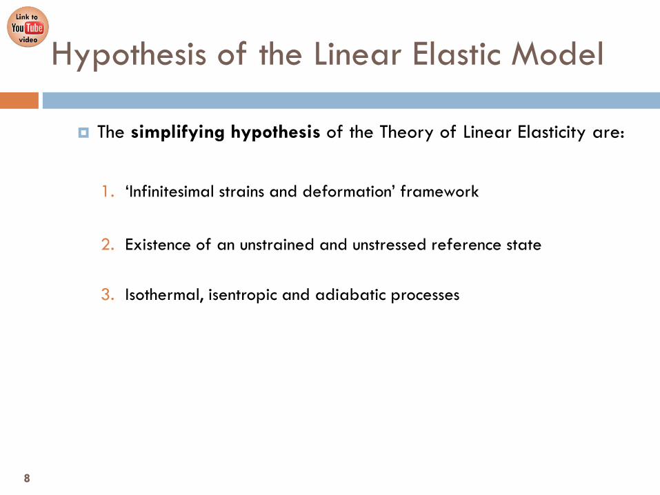
The simplifying hypothesis of the Theory of Linear Elasticity are:
1. ‘Infinitesimal strains and deformation’ framework
2. Existence of an unstrained and unstressed reference state
3. Isothermal, isentropic and adiabatic processes
8
Hypothesis of the Linear Elastic Model
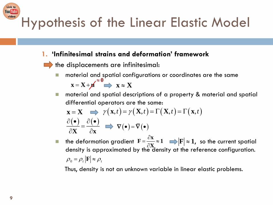
1. ‘Infinitesimal strains and deformation’ framework the displacements are infinitesimal: material and spatial configurations or coordinates are the same
material and spatial descriptions of a property & material and spatial
differential operators are the same:
the deformation gradient , so the current spatial density is approximated by the density at the reference configuration.
Thus, density is not an unknown variable in linear elastic problems.
≈x X
( ) ( ) ( ) ( ), , , ,t t t tγ γ= = Γ = Γx X X x( ) ( )∂ • ∂ •
=∂ ∂X x
∂= ≈
∂xF 1X
0 t tρ ρ ρ= ≈F
=x X
( ) ( )• = •∇ ∇
≈F 1
= +x X u≈ 0
9

Hypothesis of the Linear Elastic Model
1. ‘Infinitesimal strains and deformation’ framework the displacement gradients are infinitesimal: The strain tensors in material and spatial configurations collapse
into the infinitesimal strain tensor. ( ) ( ) ( ), , ,t t t≈ =E X e x xε
10

Hypothesis of the Linear Elastic Model
2. Existence of an unstrained and unstressed reference state It is assumed that there exists a reference unstrained and unstressed
neutral state, such that,
The reference state is usually assumed to correspond to the reference configuration.
11
( ) ( )( ) ( )
0 0
0 0
,
,
t
t
= =
= =
x x 0
x x 0
ε ε
σ σ

3. Isothermal and adiabatic (=isentropic) processes In an isothermal process the temperature remains constant.
In an isentropic process the entropy of the system remains constant.
In an adiabatic process the net heat transfer entering into the body is zero.
Hypothesis of the Linear Elastic Model
( ) ( ) ( )0 0, ,t tθ θ θ≡ ≡ ∀x x x x
( , ) ( ) 0dss t sdt
= = =X X
e 0Q 0V V
r dV dS V Vρ∂
= − ⋅ = ∀∆ ⊂∫ ∫ q n
0 0r tρ − ⋅ = ∀ ∀q x∇
0s =
heat conduction from the exterior
internal sources
12
REMARK An isentropic process is an idealized thermodynamic process that is adiabatic, isothermal and reversible.

13
Ch.6. Linear Elasticity
6.2 Linear Elastic Constitutive Equation

R. Hooke observed in 1660 that, for relatively small deformations of an object, the displacement or size of the deformation is directly proportional to the deforming force or load.
Hooke’s Law (for 1D problems) states that in an elastic material strain is directly proportional to stress through the elasticity modulus.
Hooke’s Law
Eσ = ε
σ
ε
E
F
F k l= ∆F lEA l
∆=
14

This proportionality is generalized for the multi-dimensional case in the Theory of Linear Elasticity.
It constitutes the constitutive equation of a linear elastic material. The 4th order tensor is the constitutive elastic constants tensor:
Has 34=81 components. Has the following symmetries, reducing the tensor to 21 independent
components:
Generalized Hooke’s Law
( ) ( )
, ( ) ,
, 1, 2,3ij ijkl kl
t t
i jσ ε
= = ∈
x x : xσ εC
CGeneralized Hooke’s Law
ijkl jikl
ijkl ijlk
=
=
C CC C
minor symmetries
ijkl klij=C Cmajor symmetries
REMARK The current stress at a point depends only on the current strain at the point, and not on the past history of strain states at the point.
15

The internal energy balance equation for the (adiabatic) linear elastic model is
Where: is the specific internal energy (energy per unit mass). is the specific heat generated by the internal sources. is the heat conduction flux vector per unit surface.
Elastic Potential
( )0 :d u rdt
ρ ρ= + − ∇ ⋅qεσ
global form
local form
( )00 0
V V V V
d d uu dV dV dV r dVdt dt
ρρ ρ=
= = + − ∇ ⋅∫ ∫ ∫ ∫: d q
σε
qru
REMARK The rate of strain tensor is related to the material derivative of the material strain tensor through: In this case, and .
T= ⋅ ⋅E F d F
=E ε =F 1
stress power heat transfer rate
infinitesimal strains
( )V V tt ≡ ∀
internal energy
16

The stress power per unit of volume is an exact differential of the internal energy density, , or internal energy per unit of volume:
Operating in indicial notation:
Elastic Potential
0ˆ( , ) ˆ( ) :
ˆ
d du tu udt dtu
ρ = = =x
σ ε
u
( ))
:
: :
ˆ 1 ( )2
1 1( )2 2
12
ij ij ij ijkl kl ij ijkl kl ij ijkl kl
ij ijkl kl kl klij ij ij ijkl kl ij ijkl kl
ij ijkl kl
ijkl kl
jklij ijkl kl
i
i kj l
ddt
dudt
ddt
ε
ε
(
↔↔
ε ε
= = ε σ = ε ε = ε ε + ε ε =
= ε ε + ε = ε ε + ε ε =
= ε ε
:
ε
ε ε
σ εC
C
C
CC
C C C
C C C C
C
REMARK The symmetries of the constitutive elastic constants tensor are used:
ijkl jikl
ijkl ijlk
=
=
C CC C
minor symmetries
ijkl klij=C Cmajor symmetries
( )ˆ 12
du ddt dt
= : :Cε ε
17

Consequences: 1. Consider the time derivative of the internal energy in the whole
volume:
In elastic materials we talk about deformation energy because the stress power is an exact differential.
Elastic Potential
( )ˆ 1: : :2
du ddt dt
= = Cσ ε ε ε
( ) ( ) ( )ˆˆ ˆ, , :V V V
d d du t dV u t dV t dVdt dt dt
= = =∫ ∫ ∫x x σ εU stress power
REMARK The stress power, in elastic materials is an exact differential of the internal energy . Then, in elastic processes, we can talk of the elastic energy .
18
ˆU
ˆ( )tU
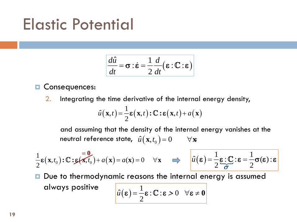
Consequences: 2. Integrating the time derivative of the internal energy density,
and assuming that the density of the internal energy vanishes at the neutral reference state, :
Due to thermodynamic reasons the internal energy is assumed
always positive
Elastic Potential
( ) ( ) ( )0 01 , , ( ) 02
t t a a+ = = ∀x : : x x x xCε ε
( ) ( ) ( ) ( )1ˆ , , ,2
u t t t a= +x x : : x xCε ε
( )0ˆ , 0u t = ∀x x
= 0
( ) 1ˆ : : 02
u = ∀ ≠ 0Cε ε ε ε>
( )
1 1ˆ : : ( ) :2 2
u = =Cε ε ε σ ε εσ
19
( )ˆ 1: : :2
du ddt dt
= = Cσ ε ε ε

The internal energy density defines a potential for the stress tensor, and is thus, named elastic potential. The stress tensor can be computed as
The constitutive elastic constants tensor can be obtained as the
second derivative of the internal energy density with respect to the strain tensor field,
Elastic Potential
( )2 ˆijkl
ij kl
u∂=
∂ε ∂εε
C
( )u∂=
∂ε
σε
( ) ( )2 ˆ :( ) u∂ ∂∂= = =
∂ ∂ ⊗ ∂ ∂C
Cε εσ ε
ε ε ε ε
ˆ( ( , )) 1 1 1 1( : : : : ( )2 2 2 2
u t∂ ∂= = + = + =
∂ ∂xε
ε ε) ε ε σ σ σε ε
C C C= σ
T= =σ σ
20
( ) ( ), ( ) ,t t=x x : xσ εC

21
Ch.6. Linear Elasticity
6.3 Isotropic Linear Elasticity

An isotropic elastic material must have the same elastic properties (contained in ) in all directions. All the components of must be independent of the orientation of the
chosen (Cartesian) system must be a (mathematically) isotropic tensor.
Where: is the 4th order unit tensor defined as and are scalar constants known as Lamé‘s parameters or coefficients.
Isotropic Constitutive Elastic Constants Tensor
( ) 2
, , , 1, 2,3ijkl ij kl ik jl il jk i j k l
λ µ
λδ δ µ δ δ δ δ
= ⊗ + = + + ∈
IC
C
1 1
CC
C
REMARK The isotropy condition reduces the number of independent elastic constants from 21 to 2.
[ ] 12 ik jl il jkijkl
δ δ δ δ = + IIλ µ
22

Introducing the isotropic constitutive elastic constants tensor into the generalized Hooke’s Law , in index notation:
And the resulting constitutive equation is,
Isotropic Linear Elastic Constitutive Equation
( )( )1 12 ( ) 22 2
ij ijkl kl ij kl ik jl il jk kl
ij kl kl ik jl kl il jk kl ij ijTr
σ ε λδ δ µ δ δ δ δ
λδ δ µ δ δ δ δ λ δ µ
= = + + ε =
= ε + ε + ε = + ε
ε
C
2λ µ= ⊗ + IC 1 1 = :Cσ ε
( )
2
2 , 1,2,3ij ij ll ij
Tr
i j
λ µ
σ λδ ε µ ε
= +
= + ∈
σ ε ε1 Isotropic linear elastic constitutive equation.
Hooke’s Law
( )ll Tr= =ε ε ji ij= =ε ε
ij= ε
12
12 i jij j i+= =ε ε ε
23

If the constitutive equation is,
Then, the internal energy density can be reduced to:
Elastic Potential
( )
2
2 , 1, 2,3ij ij ll ij
Tr
i j
λ µ
σ λδ ε µ ε
= +
= + ∈
σ ε ε1 Isotropic linear elastic constitutive equation.
Hooke’s Law
( ) ( )
( )( )
( )2
1 1ˆ : ( ) 2 :2 2
1 1: 22 2
12
Tr
u Tr
Tr
Tr
λ µ
λ µ
λ µ
= +
+
= +
=σ
ε
ε ε = ε ε ε =
= ε ε ε : ε =
ε ε : ε
σ 1
1
REMARK The internal energy density is an elastic potential of the stress tensor as:
( ) ( ) ( )ˆ
2u
Trλ µ∂
= = +∂
ε εε
σ εε
1
24

1. is isolated from the expression derived for Hooke’s Law
2. The trace of is obtained:
3. The trace of is easily isolated:
4. The expression in 3. is introduced into the one obtained in 1.
Inversion of the Constitutive Equation
( ) ( )( ) ( ) ( ) ( ) ( ) ( )2 2 3 2Tr Tr Tr Tr Tr Tr Trλ µ λ µ λ µ= + + = +σ ε ε = ε ε ε1 1
σ
( ) ( )13 2
Tr Trλ µ
=+
ε σ
ε
ε
( ) 2Trλ µ= +σ ε ε1 ( )( )12
Trλµ
ε = σ − ε 1
( )1 12 3 2
Trλµ λ µ
+
ε = σ − σ 1( ) ( ) 1
2 3 2 2Trλ
µ λ µ µ+
+ε = − σ σ1
=3
25

The Lamé parameters in terms of and :
So the inverse const. eq. is re-written:
Inverse Isotropic Linear Elastic Constitutive Equation
( )( )( )( )
( )( )
1 1
1 1
1 1
x x y z xy xy
y y x z xz xz
z z x y yz yz
E G
E G
E G
ε σ ν σ σ γ τ
ε σ ν σ σ γ τ
ε σ ν σ σ γ τ
= − + =
= − + =
= − + =
( )
1
1 , 1,2,3ij ll ij ij
TrE E
i jE E
ν ν
ν νε σ δ σ
+ = − + + = − + ∈
ε σ σ1
νE
Inverse isotropic linear elastic constitutive equation.
Inverse Hooke’s Law.
( )
( )
3 2
2
Eµ λ µ
λ µλν
λ µ
+=
+
=+
( )( )
( )
1 1 2
2 1
E
EG
νλν ν
µν
=+ −
= =+
In engineering notation:
26
( ) ( ) 12 3 2 2
Trλµ λ µ µ
++
ε = − σ σ1

Young's modulus is a measure of the stiffness of an elastic material. It is given by the ratio of the uniaxial stress over the uniaxial strain.
Poisson's ratio is the ratio, when a solid is uniaxially stretched, of the transverse strain (perpendicular to the applied stress), to the axial strain (in the direction of the applied stress).
Young’s Modulus and Poisson’s Ratio
ν
E
( )3 2E
µ λ µλ µ
+=
+
( )2λν
λ µ=
+
27

Example
Consider an uniaxial traction test of an isotropic linear elastic material such that:
Obtain the strains (in engineering notation) and comment on the results obtained for a Poisson’s ratio of and .
xσ xσ
x
y
z
xσxσ
00
x
y z xy xz yz
σσ σ τ τ τ
>= = = = =
E, ν
0ν = 0.5ν =
28

Solution
For :
For :
0ν =1 0
0
0
x x xy
y x xz
z x yz
E
E
E
ε σ γ
νε σ γ
νε σ γ
= =
= − =
= − =
1 0
0 00 0
x x xy
y xz
z yz
Eε σ γ
ε γε γ
= =
= == =
0.5ν =
1 0
0.5 0
0.5 0
x x xy
y x xz
z x yz
E
E
E
ε σ γ
ε σ γ
ε σ γ
= =
= − =
= − =
1 0
1 021 0
2
x x xy
y x xz
z x yz
E
E
E
ε σ γ
ε σ γ
ε σ γ
= =
= − =
= − =
There is no Poisson’s effect and the transversal normal strains are zero.
The volumetric deformation is zero, , the material is incompressible and the volume is preserved.
tr 0x y zε ε ε= + + =ε
29
( )( )( )( )
( )( )
1 1
1 1
1 1
x x y z xy xy
y y x z xz xz
z z x y yz yz
E G
E G
E G
ε σ ν σ σ γ τ
ε σ ν σ σ γ τ
ε σ ν σ σ γ τ
= − + =
= − + =
= − + =
00
x
y z xy xz yz
σσ σ τ τ τ
>= = = = =

The stress tensor can be split into a spherical, or volumetric, part and a deviatoric part:
Similarly for the strain tensor:
Spherical and deviatoric parts of Hooke’s Law
( )1:3sph m Trσ= =σ σ1 1
dev mσ′ = = 1σ σ σ −mσ ′= +σ σ1
1 ´3
e= +ε ε1
1 1 Tr (3 3sph e= = )ε ε1 1
1dev3
e′ = =ε ε ε− 1
30

Operating on the volumetric strain:
The spherical parts of the stress and strain tensor are directly related:
Spherical and deviatoric parts of Hooke’s Law
( )Tre = ε
( ) 1TrE Eν ν+
= − +ε σ σ1
( ) ( ) ( )1Tr Tr TreE Eν ν+
= − +σ σ1
( )3 1 2me
Eν
σ−
=
3= 3 mσ=
( )3 1 2mE eσ
ν=
−
: bulk modulus (volumetric strain modulus) K
23 3(1 2 )
def EK λ µν
= + =−
m K eσ =
31

Introducing into :
Taking into account that :
The deviatoric parts of the stress and strain tensor are related component by component:
Spherical and Deviator Parts of Hooke’s Law
mσ ′= +σ σ1
( )3 1 2mE eσ
ν=
−
( ) 1TrE Eν ν+
= − +ε σ σ1
( ) ( )
( ) ( )
1
1 1 1 3 1
m m
m m m
TrE E
Tr TrE E E E E E E
ν νσ σ
ν ν ν ν ν ν νσ σ σ
+′ ′= − + + +
+ + + + ′ ′ ′= − − + + = − +
ε σ σ
σ σ σ
1 1 1
1 1 1 1 13=
( )1 2 1 1 1 1
3 1 2 3E e e
E E Eν ν ν
ν− + + ′ ′= + = + −
ε σ σ1 1
0=
2 2 , 1,2,3ij ijG G i jσ ε′ ′ ′ ′= = ∈εσ
1 ´3
e= +ε ε1
Comparing this with the expression
1´E
ν+ ′=ε σ1 1 1
E 2 2Gν
µ+
= =
32
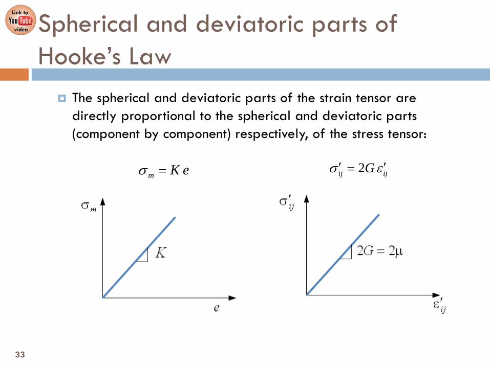
The spherical and deviatoric parts of the strain tensor are directly proportional to the spherical and deviatoric parts (component by component) respectively, of the stress tensor:
Spherical and deviatoric parts of Hooke’s Law
2ij ijGσ ε′ ′=m K eσ =
33
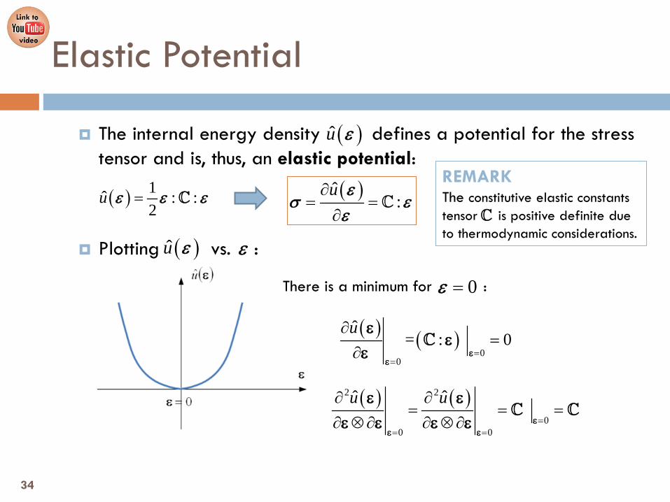
The internal energy density defines a potential for the stress tensor and is, thus, an elastic potential:
Plotting vs. :
Elastic Potential
( ) 1ˆ : :2
u = Cε ε ε ( )ˆ:
u∂= =
∂
εσ ε
ε
( )u ε
( ) ( )2 2
00 0
ˆ ˆu u=
= =
∂ ∂= = =
∂ ⊗ ∂ ∂ ⊗ ∂C C
εε ε
ε εε ε ε ε
( )u ε ε
( ) ( )0
0
ˆ= : 0
u=
=
∂=
∂C
εε
εε
ε
There is a minimum for : 0=ε
REMARK The constitutive elastic constants tensor is positive definite due to thermodynamic considerations.
C
34

The elastic potential can be written as a function of the spherical and deviatoric parts of the strain tensor:
Elastic Potential
( ) 1 1ˆ2 2
: : :u = =ε ε ε σ εC
( ) ( )21 1: : :2 2
Tr Trλ µ λ µ= + = +ε ε ε ε ε ε ε1
( ): : : : :=ε ε ε ε = σ εC C
( )1 22
Trλ µ= + :ε ε ε =1
σ=
( )Tr e= =ε 2e=
( )
2
2
03
1 1´ ´3 31 2 ´ ´ ´9 3
1 ´ ´3
Tr
e e
e e
e
′ =
= + + =
= + + =
= +
:
: : :
:
ε
ε ε
ε ε ε
ε ε
1 1
1 1 1
( ) 2 2 21 1 1 2ˆ : ´ : ´2 3 2 3
u e e μ e μλ µ λ µ = + + = + +
ε ε ε ε ε
K
( ) 21ˆ : ´ 02
u K e µ= + ≥ε ε εElastic potential in terms of the spherical and deviatoric parts of the strains.
35

The derived expression must hold true for any deformation process:
Consider now the following particular cases of isotropic linear elastic material: Pure spherical deformation process
Pure deviatoric deformation process
Limits in the Elastic Properties
( ) 21ˆ : : ´ 02
u K e µ= + ≥ε ε ε´
( )
( )
1
1
13
e=
′ = 0
ε
ε
1 ( )1 21ˆ 02
u K e= ≥ 0K >
( )
( )
2
2e
′=
= 0
ε ε ( )2ˆ ´ ´ 0u µ= ≥:ε ε 0µ >
: 0ij ijε ε′ ′ = ≥ε εREMARK
bulk modulus
Lamé’s second parameter
36
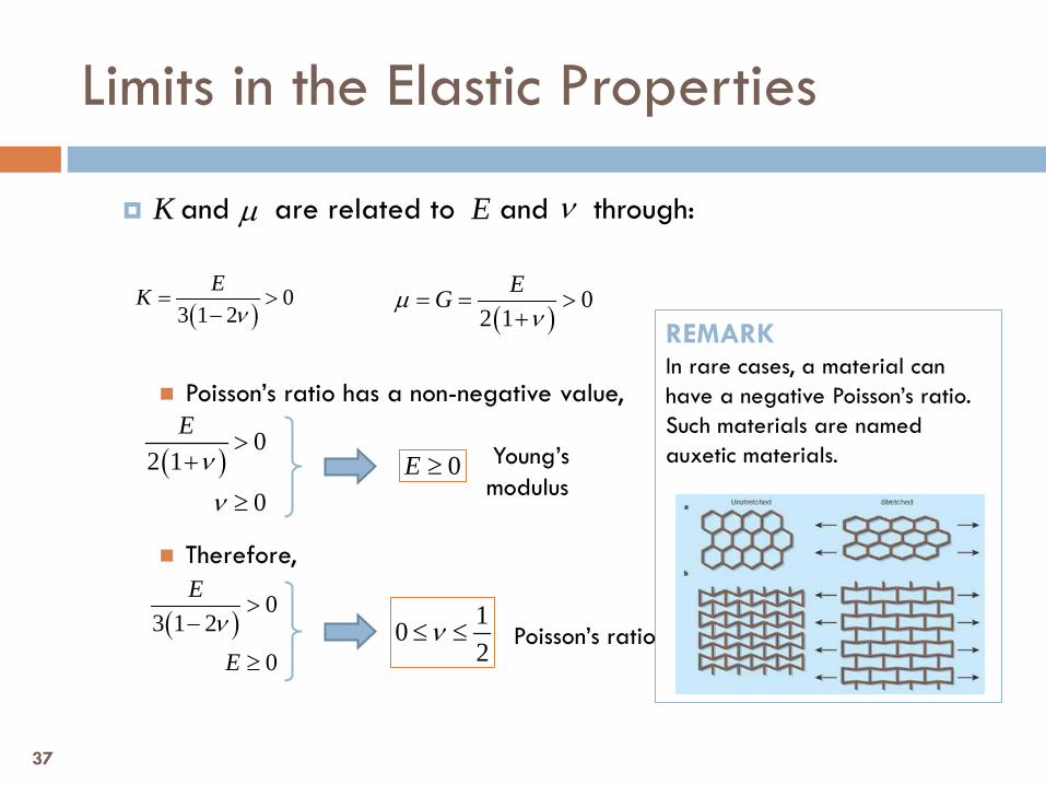
and are related to and through: Poisson’s ratio has a non-negative value,
Therefore,
Limits in the Elastic Properties
K µ E ν
( )0
3 1 2EK
ν= >
− ( )0
2 1EGµ
ν= = >
+
( )0
2 10
Eνν
>+
≥0E ≥ Young’s
modulus
( )0
3 1 20
E
Eν
>−
≥
102
ν≤ ≤ Poisson’s ratio
REMARK In rare cases, a material can have a negative Poisson’s ratio. Such materials are named auxetic materials.
37
38
Ch.6. Linear Elasticity
6.4 The Linear Elastic Problem
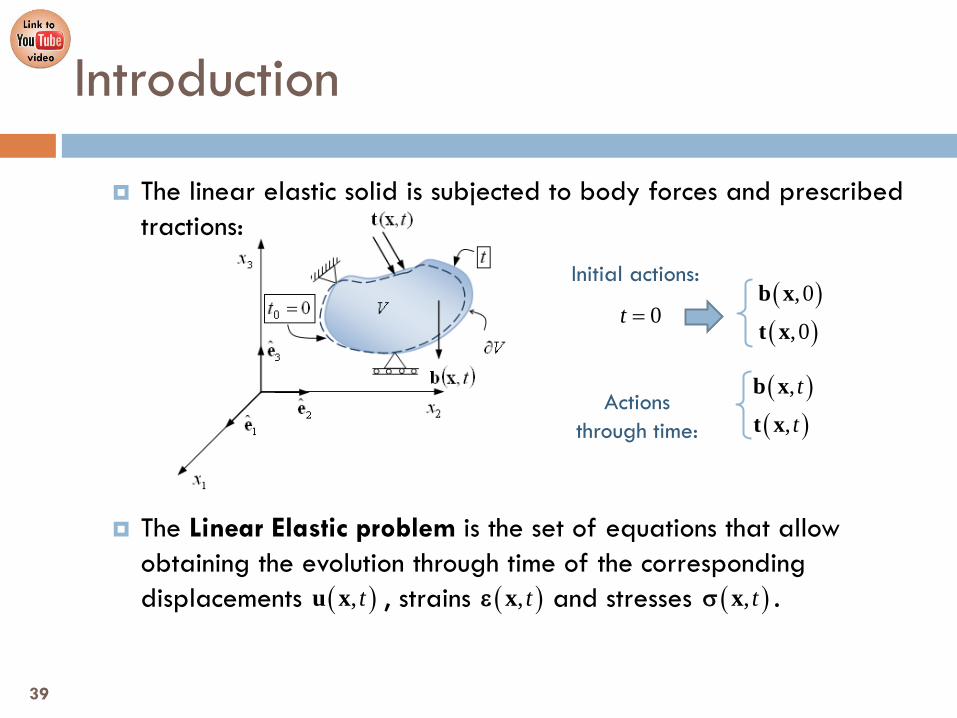
The linear elastic solid is subjected to body forces and prescribed tractions:
The Linear Elastic problem is the set of equations that allow obtaining the evolution through time of the corresponding displacements , strains and stresses .
Introduction
0t =( )( )
,0
,0
b x
t x
( )( )
,
,
t
t
b x
t x
Initial actions:
Actions through time:
( ), tu x ( ), txε ( ), txσ
39

The Linear Elastic Problem is governed by the equations: 1. Cauchy’s Equation of Motion. Linear Momentum Balance Equation.
2. Constitutive Equation. Isotropic Linear Elastic Constitutive Equation.
3. Geometrical Equation. Kinematic Compatibility.
Governing Equations
( ) ( ) ( )2
0 0 2
,, ,
tt t
tρ ρ
∂⋅ + =
∂u x
x b x∇ σ
( ) ( ), 2t Trλ µ= +xσ ε ε1
( ) ( ) ( )1, ,2
St t= = ⊗ + ⊗x u x u uε ∇ ∇ ∇
This is a PDE system of 15 eqns -15 unknowns: Which must be solved in the space.
( ), tu x( ), txε
( ), txσ
3 unknowns
6 unknowns
6 unknowns
3+×R R
40

Boundary conditions in space Affect the spatial arguments of the unknowns Are applied on the boundary of the solid, which is divided into three parts:
Prescribed displacements on :
Prescribed tractions on :
Prescribed displacements and stresses on :
Boundary Conditions
Γ
0u u
u u u u
Vσ σ
σ σ σ σ
Γ Γ Γ = Γ ≡ ∂
Γ Γ = Γ Γ = Γ Γ = /
uΓ
σΓ
uσΓ
( ) ( )
*
*
( , ) ( , ), , 1, 2,3 u
i i
t tt
u t u t i = ∀ ∈Γ ∀ = ∈
u x u xx
x x
( ) ( )
*
*
( , ) ( , ), , 1,2,3ij j j
t tt
t n t t i σσ ⋅ = ∀ ∈ Γ ∀ ⋅ = ∈
x n xx
x xσ t
( ) ( )( ) ( ) ( )
*
*
, ,, , 1, 2,3
, ,i i
ujk k j
u t u ti j k i j t
t n t t σσ = ∈ ≠ ∀ ∈Γ ∀ ⋅ =
x xx
x x
41

Boundary Conditions
42

Boundary conditions in time. INTIAL CONDITIONS. Affect the time argument of the unknowns. Generally, they are the known values at :
Initial displacements:
Initial velocity:
Boundary Conditions
0t =
( ),0 V= ∀ ∈u x 0 x
( ) ( ) ( )00
,,0
not
t
tV
t=
∂= = ∀ ∈
∂u x
u x v x x
43

Find the displacements , strains and stresses such that
The Linear Elastic Problem
( ), tu x ( ), txε ( ), txσ
( ) ( ) ( )2
0 0 2
,, ,
tt t
tρ ρ
∂⋅ + =
∂u x
x b x∇ σ
( ) ( ), 2t Trλ µ= +xσ ε ε1
( ) ( ) ( )1, ,2
St t= = ⊗ + ⊗x u x u uε ∇ ∇ ∇
Cauchy’s Equation of Motion
Constitutive Equation
Geometric Equation
*
*
:
:u
σ
Γ =
Γ = ⋅
u ut nσ Boundary conditions in space
( )( ) 0
,0
,0
=
=
u x 0
u x v
Initial conditions (Boundary conditions in time)
44

The linear elastic problem can be viewed as a system of actions or data inserted into a mathematical model made up of the EDP’s and boundary conditions , which gives a response (or solution) in displacements, strains and stresses.
Generally, actions and responses depend on time. In these cases, the problem is a dynamic problem, integrated in .
In certain cases, the integration space is reduced to . The problem is termed quasi-static.
Actions and Responses
( )( )( )( )
*
*
0
,,,
ttt
b xt xu xv x
( )( )( )
,,,
ttt
u xxx
εσ
( )not
, t= xAACTIONS ( )
not, t= xRRESPONSES
Mathematical model
EDPs+BCs
3+×R R
3R
45

A problem is said to be quasi-static if the acceleration term can be considered to be negligible. This hypothesis is acceptable if actions are applied slowly. Then,
The Quasi-Static Problem
2
2
( , )tt
∂= ≈
∂u xa 0
2 2/ t∂ ∂ ≈ 0A 2 2/ t∂ ∂ ≈ 0R2
2
( , )tt
∂≈
∂u x 0
46

Find the displacements , strains and stresses such that
( )2
0 2
, tt
ρ∂
≈∂u x
0
The Quasi-Static Problem
( ), tu x ( ), txε ( ), txσ
( ) ( )0, ,t tρ⋅ + =x b x 0∇ σ
( ) ( ), 2t Trλ µ= +xσ ε ε1
( ) ( ) ( )1, ,2
St t= = ⊗ + ⊗x u x u uε ∇ ∇ ∇
*
*
:
:u
σ
Γ =
Γ = ⋅
u ut nσ
( )( ) 0
,0
,0
=
=
u x 0
u x v
Equilibrium Equation
Constitutive Equation
Geometric Equation
Boundary Conditions in Space
Initial Conditions
47

The quasi-static linear elastic problem does not involve time derivatives. Now the time variable plays the role of a loading descriptor: it describes the
evolution of the actions.
For each value of the actions -characterized by a fixed value - a response is obtained.
Varying , a family of actions and its corresponding family of responses are obtained.
The Quasi-Static Problem
( )( )( )
*
*
,,,
λλλ
b xt xu x
( )( )( )
,,,
λλλ
u xxx
εσ
( )not
,λ= xAACTIONS ( )not
,λ= xRRESPONSES
Mathematical model
EDPs+BCs
*λ( )*,λxA( )*,λxR
*λ
48

Consider the typical material strength problem where a cantilever beam is subjected to a force at it’s tip.
For a quasi-static problem,
The response is , so for every time instant, it only depends on the corresponding value .
Example
( )F t
( ) (( ))t tδ δλ=( )tλ
49

To solve the isotropic linear elastic problem posed, two approaches can be used: Displacement formulation - Navier Equations Eliminate and from the general system of equations. This
generates a system of 3 eqns. for the 3 unknown components of . Useful with displacement BCs. Avoids compatibility equations. Mostly used in 3D problems. Basis of most of the numerical methods.
Stress formulation - Beltrami-Michell Equations. Eliminates and from the general system of equations. This
generates a system of 6 eqns. for the 6 unknown components of . Effective with boundary conditions given in stresses. Must work with compatibility equations. Mostly used in 2D problems. Can only be used in the quasi-static problem.
Solution of the Linear Elastic Problem
( ), tu x( ), txε( ), txσ
( ), tu x ( ), txε( ), txσ
50
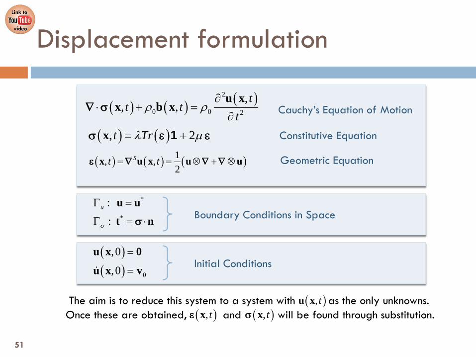
The aim is to reduce this system to a system with as the only unknowns. Once these are obtained, and will be found through substitution.
Displacement formulation
( ) ( ) ( )2
0 0 2
,, ,
tt t
tρ ρ
∂⋅ + =
∂u x
x b x∇ σ
( ) ( ), 2t Trλ µ= +xσ ε ε1
( ) ( ) ( )1, ,2
St t= = ⊗ + ⊗x u x u uε ∇ ∇ ∇
Cauchy’s Equation of Motion
Constitutive Equation
Geometric Equation
*
*
:
:u
σ
Γ =
Γ = ⋅
u ut nσ Boundary Conditions in Space
( )( ) 0
,0
,0
=
=
u x 0
u x v
Initial Conditions
( ), tu x( ), txε ( ), txσ
51

Introduce the Constitutive Equation into Cauchy’s Equation of motion: Consider the following identities:
Displacement formulation
( ) ( ) ( )2
0 0 2
,, ,
tt t
tρ ρ
∂⋅ + =
∂u x
x b x∇ σ
( ) ( ), 2t Trλ µ= +xσ ε ε1[ ]
2
0 0 2( ) 2Trt
λ µ ρ ρ ∂⋅ + ⋅ + =
∂ub∇ ε ∇ ε1
( ) ( ) ( )
( )
11( )
1,2,3
k kij iji
j j k i k i
i
u uTrx x x x x x
i
ε δ δ ∂ ∂ ∂ ∂ ∂ ∂
⋅ = = = = ⋅ = ∂ ∂ ∂ ∂ ∂ ∂
= ⋅ ∈
1 u
u
∇ ε ∇
∇ ∇
⋅= u∇
( )( )ui
⋅= ∇ ∇
( )( ) ( )Tr⋅ = ⋅u∇ ε ∇ ∇1
52

Introduce the Constitutive Equation into Cauchy’s Equation of motion: Consider the following identities:
Displacement formulation
( ) ( ) ( )2
0 0 2
,, ,
tt t
tρ ρ
∂⋅ + =
∂u x
x b x∇ σ
( ) ( ), 2t Trλ µ= +xσ ε ε1[ ]
2
0 0 2( ) 2Trt
λ µ ρ ρ ∂⋅ + ⋅ + =
∂ub∇ ε ∇ ε1
( ) ( ) ( )
( )
2
2
21 1 1 1 12 2 2 2 2
1 1 1,2,32 2
ij j ji ii
j j j i j j i j i
i
i
u uu ux x x x x x x x x
i
ε ∂ ∂ ∂∂ ∂∂ ∂ ∂⋅ = = + = + = + ⋅ = ∂ ∂ ∂ ∂ ∂ ∂ ∂ ∂ ∂
= + ⋅ ∈
u u
u u
∇∇ ε ∇
∇ ∇ ∇
( )2
i= u∇
⋅= u∇
( )( )i⋅= u∇ ∇
21 1( )2 2
⋅ = ⋅ +u u∇ ε ∇ ∇ ∇
53
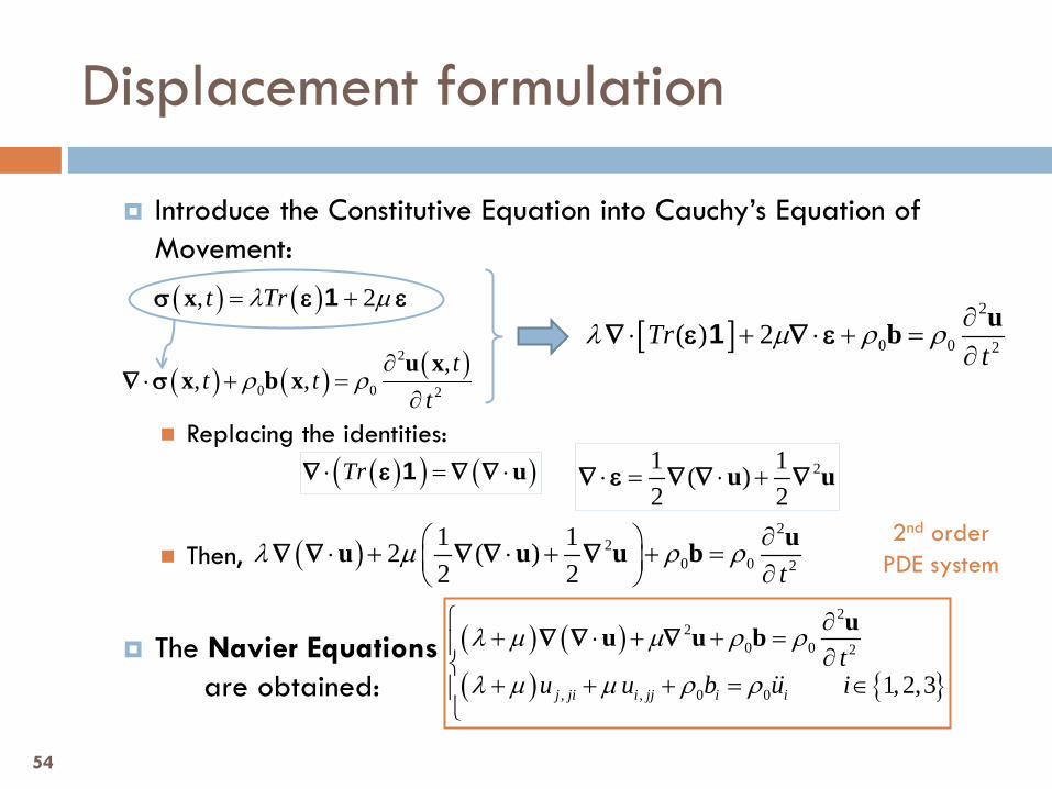
Introduce the Constitutive Equation into Cauchy’s Equation of Movement: Replacing the identities:
Then,
The Navier Equations are obtained:
Displacement formulation
( ) ( ) ( )2
0 0 2
,, ,
tt t
tρ ρ
∂⋅ + =
∂u x
x b x∇ σ
( ) ( ), 2t Trλ µ= +xσ ε ε1[ ]
2
0 0 2( ) 2Trt
λ µ ρ ρ ∂⋅ + ⋅ + =
∂ub∇ ε ∇ ε1
( )( ) ( )Tr⋅ = ⋅u∇ ε ∇ ∇1 21 1( )2 2
⋅ = ⋅ +u u∇ ε ∇ ∇ ∇
( )2
20 0 2
1 12 ( )2 2 t
λ µ ρ ρ ∂ ⋅ + ⋅ + + = ∂ uu u u b∇ ∇ ∇ ∇ ∇
( ) ( )( )
22
0 0 2
, , 0 0 1, 2,3j ji i jj i i
tu u b u i
λ µ µ ρ ρ
λ µ µ ρ ρ
∂+ ⋅ + + = ∂+ + + = ∈
uu u b
∇ ∇ ∇
2nd order PDE system
54

The boundary conditions are also rewritten in terms of :
The BCs are now:
Displacement formulation
( ), tu x
( ) ( ), 2t Trλ µ= +xσ ε ε1
* = ⋅t nσ( )( )* 2Trλ µ= + ⋅t n nε ε
⋅= u∇
( )12
S= = ⊗ + ⊗u u u∇ ∇ ∇
( ) ( )* λ µ= ⋅ + ⊗ + ⊗ ⋅t u n u u n∇ ∇ ∇
*
* 1, 2,3i iu u i
=
= ∈
u uuΓon
σΓ( ) ( )
( )
*
*. , , 1, 2,3k k i i j j j i j iu n u n u n t i
λ µ
λ µ
⋅ + ⊗ + ⊗ ⋅ =
+ + = ∈
u n u u n t∇ ∇ ∇on
REMARK The initial conditions remain the same.
55
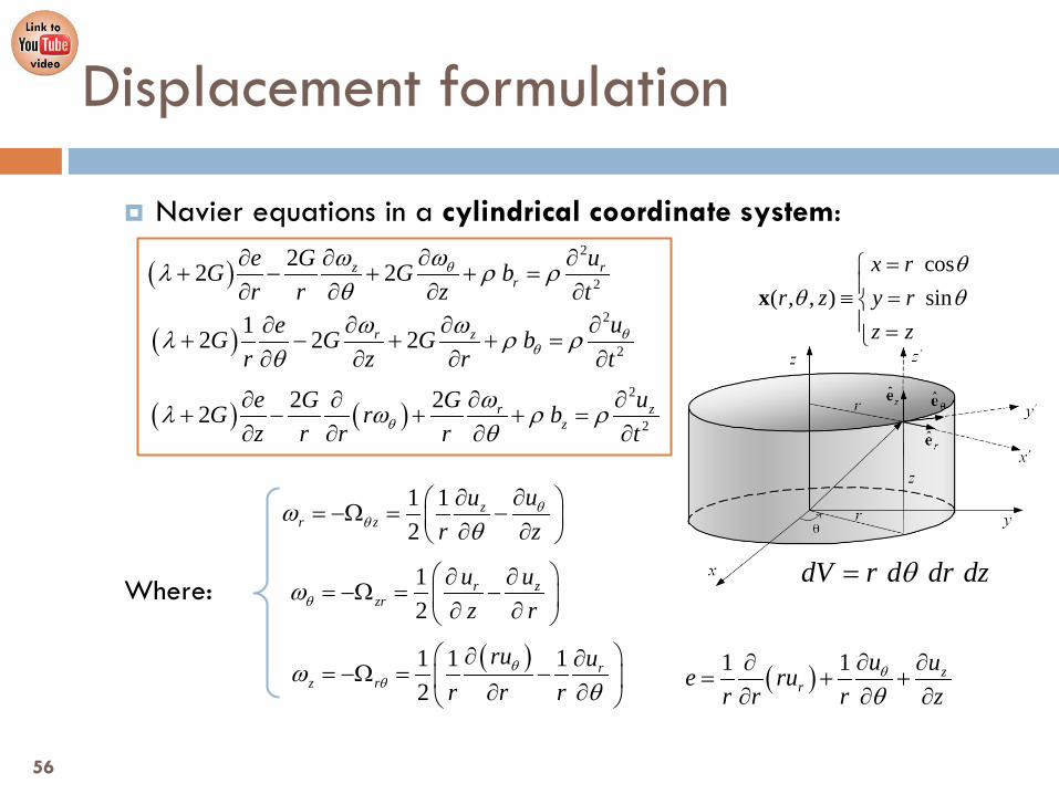
Navier equations in a cylindrical coordinate system:
Where:
Displacement formulation
cos ( , , ) sin
x rr z y r
z z
θθ θ
=≡ = =
x
dV r d dr dzθ=
( )2
2
22 2z rr
ue GG G br r z t
θωωλ ρ ρθ
∂∂ ∂∂+ − + + =
∂ ∂ ∂ ∂
( )2
2
12 2 2r z ueG G G br z r t
θθ
ω ωλ ρ ρθ
∂∂ ∂∂+ − + + =
∂ ∂ ∂ ∂
( ) ( )2
2
2 22 r zz
ue G GG r bz r r r tθ
ωλ ω ρ ρθ
∂ ∂∂ ∂+ − + + =
∂ ∂ ∂ ∂
1 12
zr z
uur z
θθω
θ∂∂ = −Ω = − ∂ ∂
12
r zzr
u uz rθω
∂ ∂= −Ω = − ∂ ∂
( )1 1 12
rz r
ru ur r r
θθω
θ∂ ∂
= −Ω = − ∂ ∂ ( )1 1 z
ru ue ru
r r r zθ
θ∂ ∂∂
= + +∂ ∂ ∂
56

Navier equations in a spherical coordinate system:
Where:
Displacement formulation
( )sin cos
, , sin sin cos
x rr y r
z r
θ ϕθ ϕ θ ϕ
θ
== ≡ = =
x x
2 sin dV r dr d dθ θ ϕ=
( ) ( )2
2
2 22 sinsin sin
rr
ue G GG br r r t
θϕ
ωλ ω θ ρ ρθ θ θ ϕ
∂ ∂∂ ∂+ − + + =
∂ ∂ ∂ ∂
( ) ( )2
2
2 2 2 sinsin sin
rG ue G G r br r r r t
θϕ θ
λ ω ω θ ρ ρθ θ ϕ θ
+ ∂∂∂ ∂− + + =
∂ ∂ ∂ ∂
( ) ( )2
2
2 2 2sin
r uG e G Gr br r r r t
ϕθ ϕ
λ ωω ρ ρθ ϕ θ
∂+ ∂∂ ∂− + + =
∂ ∂ ∂ ∂
( )1 1 1ω sin θ2 sinθ θ sin θ φr
uur r
θθϕ ϕ
∂∂= −Ω = − ∂ ∂
( )1 1 1ω2 sinθ φ
rr
ruur r r
ϕθ ϕ
∂∂ = −Ω = − ∂ ∂
( )1 1 1ω2 θ
rr
urur r rϕ θ θ
∂∂ = −Ω = − ∂ ∂
( ) ( ) ( )22
1 sin sinsin re r u ru ru
r r θ ϕθ θθ θ ϕ
∂ ∂ ∂= + + ∂ ∂ ∂
57

The aim is to reduce this system to a system with as the only unknowns. Once these are obtained, will be found through substitution and by
integrating the geometric equations.
Stress formulation
( ) ( )0, , 0t tρ⋅ + =x b x∇ σ
( ) ( ) 1, t TrE Eν ν+
= − +xε σ σ1
( ) ( ) ( )1, ,2
St t= = ⊗ + ⊗x u x u uε ∇ ∇ ∇
Equilibrium Equation (Quasi-static problem)
Inverse Constitutive Equation
Geometric Equation
*
*
:
:u
σ
Γ =
Γ = ⋅
u ut nσ Boundary Conditions in Space
( ), txσ
REMARK For the quasi-static problem, the time variable plays the role of a loading factor.
( ), tu x( ), txε
58

Taking the geometric equation and, through successive derivations, the displacements are eliminated:
Introducing the inverse constitutive equation into the compatibility equations and using the equilibrium equation:
The Beltrami-Michell Equations are obtained:
Stress formulation
Compatibility Equations (seen in Ch.3.)
2 22 2
0 , , , 1, 2,3ij jlkl ik
k l i j j l i k
i j k lx x x x x x x x
ε εε ε∂ ∂∂ ∂+ − − = ∈
∂ ∂ ∂ ∂ ∂ ∂ ∂ ∂
1ij pp ij ijE E
ν νδ +ε = − σ + σ
0 0ijj
i
bxσ
ρ∂
+ =∂
( ) ( ) ( ) 2
00 02 1 , 1, 2,31 1
jk ikkij ij
i j k j i
bb bi j
x x x x xρρ ρσ νσ δ
ν ν
∂∂ ∂∂∇ + = − − − ∈
+ ∂ ∂ − ∂ ∂ ∂
2nd order PDE system
59
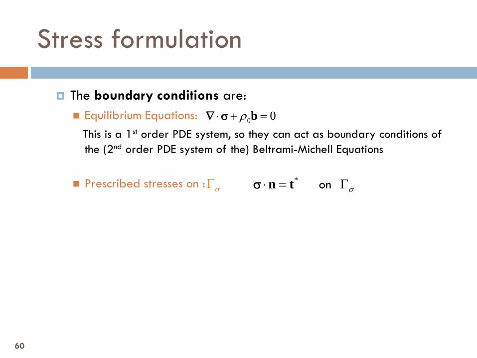
The boundary conditions are: Equilibrium Equations: This is a 1st order PDE system, so they can act as boundary conditions of
the (2nd order PDE system of the) Beltrami-Michell Equations
Prescribed stresses on :
Stress formulation
0 0ρ⋅ + =b∇ σ
σΓ *σ⋅ = Γn tσ on
60

Once the stress field is known, the strain field is found by substitution.
The calculation, after, of the displacement field requires that the geometric equations be integrated with the prescribed displacements on :
Stress formulation
REMARK This need to integrate the second system is a considerable disadvantage with respect to the displacement formulation when using numerical methods to solve the lineal elastic problem.
( )*
1( ) ( ) ( )2
( ) ( ) u
V= ⊗ + ⊗ ∈
= ∀ ∈Γ
x u x u x x
u x u x x
ε ∇ ∇uΓ
( ) ( ) 1, t TrE Eν ν+
= − +xε σ σ1
61

From A. E. H. Love's Treatise on the mathematical theory of elasticity: “According to the principle, the strains that are produced in a body by the application,
to a small part of its surface, of a system of forces statically equivalent to zero force and zero couple, are of negligible magnitude at distances which are large compared with the linear dimensions of the part.”
Expressed in another way: “The difference between the stresses caused by statically equivalent load systems is
insignificant at distances greater than the largest dimension of the area over which the loads are acting.”
Saint-Venant’s Principle
REMARK This principle does not have a rigorous mathematical proof.
( ) ( )( ) ( )( ) ( )
(I) (II)
(I) (II)
(I) (II)
, ,
, ,
, ,
P P
P P
P P
t t
t t
t t
≈
≈
≈
u x u x
x x
x x
ε ε
σ σ
|P δ∀ >>
62

Saint-Venant’s Principle
Saint Venant’s Principle is often used in strength of materials.
It is useful to introduce the concept of stress: The exact solution of this problem is very complicated.
This load system is statically equivalent to load system (I). The solution of this problem is very simple.
Saint Venant’s Principle allows approximating solution (I) by solution (II) at a far enough distance from the ends of the beam.
63

The solution of the lineal elastic problem is unique: It is unique in strains and stresses. It is unique in displacements assuming that appropriate boundary
conditions hold in order to avoid rigid body motions.
This can be proven by Reductio ad absurdum ("reduction to the
absurd"), as shown in pp. 189-193 of the course book. This proof is valid for lineal elasticity in infinitesimal strains. The constitutive tensor is used, so proof is not only valid for isotropic
problems but also for orthotropic and anisotropic ones.
Uniqueness of the solution
C
64
65
Ch.6. Linear Elasticity
6.5 Linear Thermoelasticity
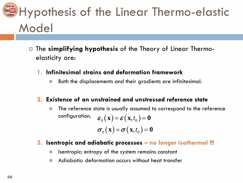
Hypothesis of the Linear Thermo-elastic Model
The simplifying hypothesis of the Theory of Linear Thermo-elasticity are:
1. Infinitesimal strains and deformation framework Both the displacements and their gradients are infinitesimal.
2. Existence of an unstrained and unstressed reference state The reference state is usually assumed to correspond to the reference
configuration.
3. Isentropic and adiabatic processes – no longer isothermal !!! Isentropic: entropy of the system remains constant Adiabatic: deformation occurs without heat transfer
( ) ( )( ) ( )
0 0
0 0
,
,
t
t
= =
= =
x x 0
x x 0
ε ε
σ σ
66

Hypothesis of the Linear Thermo-Elastic Model
3. (Hypothesis of isothermal process is removed) The process is no longer isothermal so the temperature changes
throughout time:
We will assume the temperature field is known.
But the process is still isentropic and adiabatic:
( )s t cnt≡
eQ 0V V
r dV dS V Vρ∂
= − ⋅ = ∀∆ ⊂∫ ∫ q n
0r tρ − ⋅ = ∀ ∀q x∇
0s =
heat conduction from the exterior
internal sources
( ) ( )
( ) ( )0, ,0
,, 0
nott
tt
t
θ θ θ
θθ
≠ =
∂= ≠
∂
x x
xx
67

Generalized Hooke’s Law
The Generalized Hooke’s Law becomes:
Where is the elastic constitutive tensor.
is the absolute temperature field. is the temperature at the reference state. is the tensor of thermal properties or constitutive thermal
constants tensor. It is a positive semi-definite symmetric second-order tensor.
( ) ( ) ( ) ( )( )
0
0
, : , : ,
, 1, 2,3ij ijkl kl ij
t t t
i j
θ θ θ
σ ε β θ θ
= − − = − ∆
= − − ∈
x x xC Cσ ε β ε β
CGeneralized Hooke’s Law for linear thermoelastic problems
( ), tθ x( )0 0, tθ θ= x
β
68
REMARK A symmetric second-order tensor A is positive semi-definite when zT·A·z > 0 for every non-zero column vector z.

An isotropic thermoelastic material must have the same elastic and thermal properties in all directions: must be a (mathematically) isotropic 4th order tensor:
Where: is the 4th order symmetric unit tensor defined as and are the Lamé parameters or coefficients.
is a (mathematically) isotropic 2nd order tensor:
Where: is a scalar thermal constant parameter.
Isotropic Constitutive Constants Tensors
( ) 2
, , . 1, 2,3ijkl ij kl ik jl il jk i j k l
λ µ
λδ δ µ δ δ δ δ
= ⊗ + = + + ∈
IC 1 1
C
[ ] 12 ik jl il jkijkl
δ δ δ δ = + IIλ µ
β
, 1,2,3ij ij i jββ δ
=β = ∈
β 1
β
69
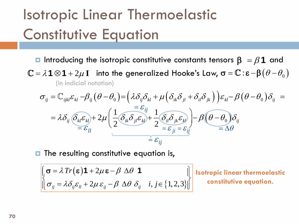
Introducing the isotropic constitutive constants tensors and into the generalized Hooke’s Law, (in indicial notation)
The resulting constitutive equation is,
Isotropic Linear Thermoelastic Constitutive Equation
( ) ( )( ) ( )
( )
0 0
01 122 2
ij ijkl kl ij ij kl ik jl il jk kl ij
ij kl kl ik jl kl il jk kl ij
σ ε β θ θ λδ δ µ δ δ δ δ ε β θ θ δ
λδ δ ε µ δ δ ε δ δ ε β θ θ δ
= − − = + + − − =
= + + − −
C
2λ µ= ⊗ + IC 1 1
( )
2
2 , 1,2,3ij ij ll ij ij
Tr
i j
λ µ β θ
σ λδ ε µ ε β θ δ
= + − ∆
= + − ∆ ∈
σ ε ε1 1 Isotropic linear thermoelastic constitutive equation.
llε= ji ijε ε= =
ijε=
ijε=
β=β 1( )0: θ θ= − −Cσ ε β
θ= ∆
70

1. is isolated from the Generalized Hooke’s Law for linear thermoelastic problems:
2. The thermal expansion coefficients tensor is defined as:
3. The inverse constitutive equation is obtained:
Inversion of the Constitutive Equation
α
ε
: θ= − ∆βσ εC1 1: :θ− −= + ∆
α
C Cε σ β
1def
−= :Cα β
It is a 2nd order symmetric tensor which involves 6 thermal expansion coefficients
1 : θ−= + ∆Cε σ α
71

For the isotropic case:
The inverse const. eq. is re-written: Where is a scalar thermal expansion coefficient related to the
scalar thermal constant parameter through:
Inverse Isotropic Linear Thermoelastic Constitutive Equation
( )
1
1 , 1,2,3ij ll ij ij ij
TrE E
i jE E
ν ν α θ
ν νε σ δ σ α θ δ
+ = − + + ∆ + = − + + ∆ ∈
ε σ σ1 1 Inverse isotropic linear thermo elastic constitutive equation.
αβ
1 2E
να β−=
72
( )
1
1
1
11 2( )
1 , , . 1, 2,3
I:
ijkl ij kl ik jl il jk
E EEi j k l
E E
ν ννβ β
ν νδ δ δ δ δ δ
−
−
−
+ = − ⊗ + − → = + = − + + ∈
CC
Cα =
1 11 1

Comparing the constitutive equations,
the decomposition is made:
Where: is the non-thermal stress: the stress produced if there is no
temperature increment. is the thermal stress: the “corrector” stress due to the
temperature increment.
Thermal Stress
( ) 2Trλ µ β θ= + − ∆σ ε ε1 1
( ) 2Trλ µ= +σ ε ε1
Isotropic linear thermoelastic constitutive equation.
Isotropic linear elastic constitutive equation.
nt= σt= σ
nt t= −σ σ σ
ntσ
tσ
73
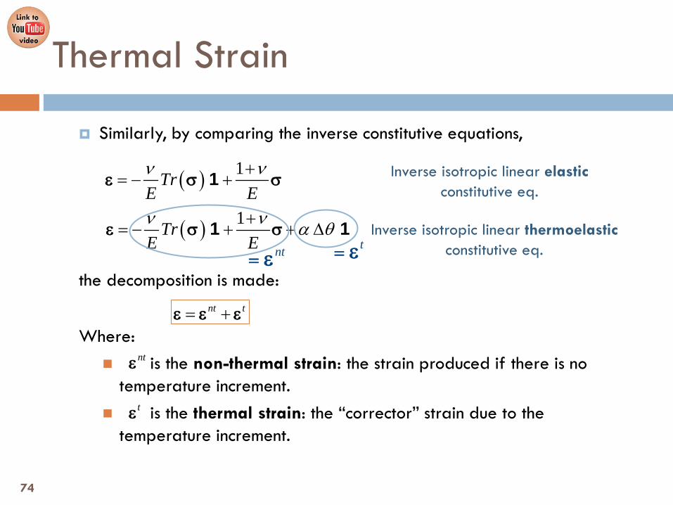
Similarly, by comparing the inverse constitutive equations,
the decomposition is made:
Where: is the non-thermal strain: the strain produced if there is no
temperature increment. is the thermal strain: the “corrector” strain due to the
temperature increment.
Thermal Strain
( ) 1TrE Eν ν α θ+
= − + + ∆ε σ σ1 1
( ) 1TrE Eν ν+
= − +ε σ σ1
Inverse isotropic linear thermoelastic constitutive eq.
Inverse isotropic linear elastic constitutive eq.
nt= εt= ε
nt t= +ε ε ε
ntε
tε
74

The thermal components appear when thermal processes are considered.
TOTAL NON-THERMAL COMPONENT
THERMAL COMPONENT
Thermal Stress and Strain
nt t= +ε ε ε
nt t= −σ σ σ
nt = :Cσ ε
1nt −= :Cε σ
t θ= ∆σ β
t θ= ∆ε α
( ) 2nt Trλ µ= +σ ε ε1 t β θ= ∆σ 1
1( )nt TrE Eν ν+
= − +ε σ σ1 t α θ= ∆ε 1
Isotropic material: Isotropic material:
Isotropic material: Isotropic material:
: :nt t = = − C Cσ ε ε ε1 1nt t− − = = + : :C Cε σ σ σ
These are the equations used in FEM codes.
75

Thermal Stress and Strain
REMARK 1 In thermoelastic problems, a state of zero strain in a body does not necessarily imply zero stress.
REMARK 2 In thermoelastic problems, a state of zero stress in a body does not necessarily imply zero strain.
nt= → =0 0ε σ
t β θ= − = − ∆ ≠ 0σ σ 1
nt= → =0 0σ ε
t α θ= = ∆ ≠ 0ε ε 1
76

77
Ch.6. Linear Elasticity
6.6 Thermal Analogies
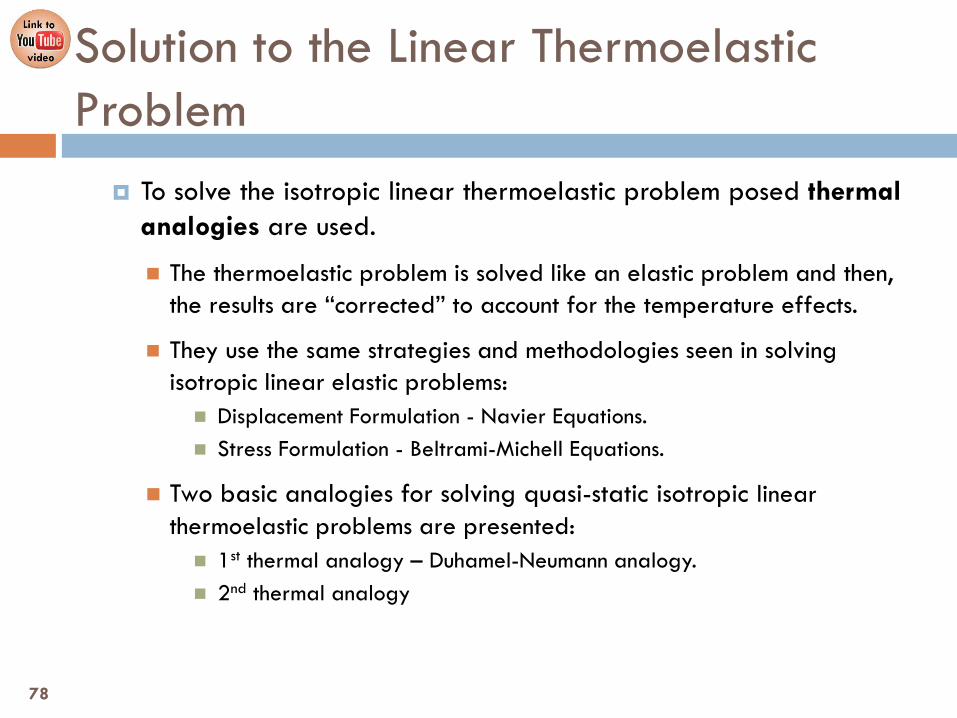
To solve the isotropic linear thermoelastic problem posed thermal analogies are used.
The thermoelastic problem is solved like an elastic problem and then, the results are “corrected” to account for the temperature effects.
They use the same strategies and methodologies seen in solving isotropic linear elastic problems: Displacement Formulation - Navier Equations. Stress Formulation - Beltrami-Michell Equations.
Two basic analogies for solving quasi-static isotropic linear thermoelastic problems are presented: 1st thermal analogy – Duhamel-Neumann analogy. 2nd thermal analogy
Solution to the Linear Thermoelastic Problem
78

1st Thermal Analogy
The governing eqns. of the quasi-static isotropic linear thermoelastic problem are:
( ) ( )0, ,t tρ⋅ + =x b x 0∇ σ
( ) ( ), ,t t β θ= − ∆x : xCσ ε 1
( ) ( ) ( )1, ,2
St t= = ⊗ + ⊗x u x u uε ∇ ∇ ∇
Equilibrium Equation
Constitutive Equation
Geometric Equation
*
*
:
:u
σ
Γ =
Γ = ⋅
u ut nσ Boundary Conditions in Space
79

1st Thermal Analogy
The actions and responses of the problem are:
( )( )( )( )
*
*
,,,
,
ttt
tθ∆
b xt x
u x
x
( )( )( )
,,,
ttt
u xxx
εσ
( ) ( )not
,I t= xAACTIONS ( ) ( )not
,I t= xRRESPONSES
Elastic model EDPs+BCs
REMARK is known a priori, i.e., it is independent of the mechanical response. This is an uncoupled thermoelastic problem.
( ), tθ∆ x
80
1st Thermal Analogy
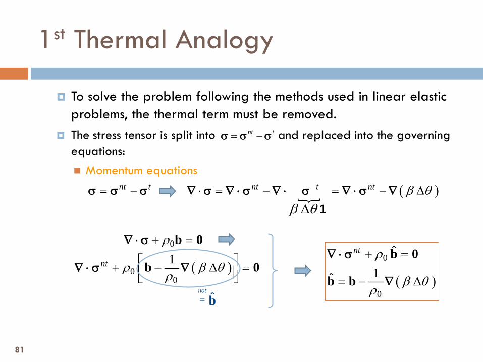
To solve the problem following the methods used in linear elastic problems, the thermal term must be removed.
The stress tensor is split into and replaced into the governing equations: Momentum equations
nt t= −σ σ σ
( )nt t nt t nt β θβ θ
= − ⋅ = − = − ∆∆
σ σ σ ∇ σ ∇ ⋅ σ ∇ ⋅ σ ∇ ⋅ σ ∇1
( )
0
0
ˆ
1ˆ
nt ρ
β θρ
+ =
= − ∆
b 0
b b
∇ ⋅ σ
∇( )
0
00
1nt
ρ
ρ β θρ
⋅ + =
+ − ∆ =
b 0
b 0
∇ σ
∇ ⋅ σ ∇
ˆnot= b
81

1st Thermal Analogy
Boundary equations:
ANALOGOUS PROBLEM – A linear elastic problem can be solved as:
0ˆnt ρ⋅ + =b 0∇ σ
( ) 2nt Trλ µ= = +:Cσ ε ε ε1
( ) ( ) ( )1, ,2
St t= = ⊗ + ⊗x u x u uε ∇ ∇ ∇
Equilibrium Equation
Constitutive Equation
Geometric Equation
0
1ˆ ( )β θρ
= − ∆b b ∇with
*
*
:ˆ:
u
ntσ
Γ =
Γ ⋅ =
u u
n tσBoundary Conditions in Space * *ˆ β θ= + ∆t t nwith
* *
*ˆ( )nt t β θ
β θ⋅ = + ⋅ = + ∆
∆ ⋅ t
n t n t nn
σ σ1
*
* *
ˆ
ˆ ( )
nt
β θ
⋅ =
= + ∆
n t
t t n
σσΓ :*
nt t= −
⋅ =n t
σ σ σ
σ*nt t⋅ − ⋅ =n n tσ σ
82
1st Thermal Analogy
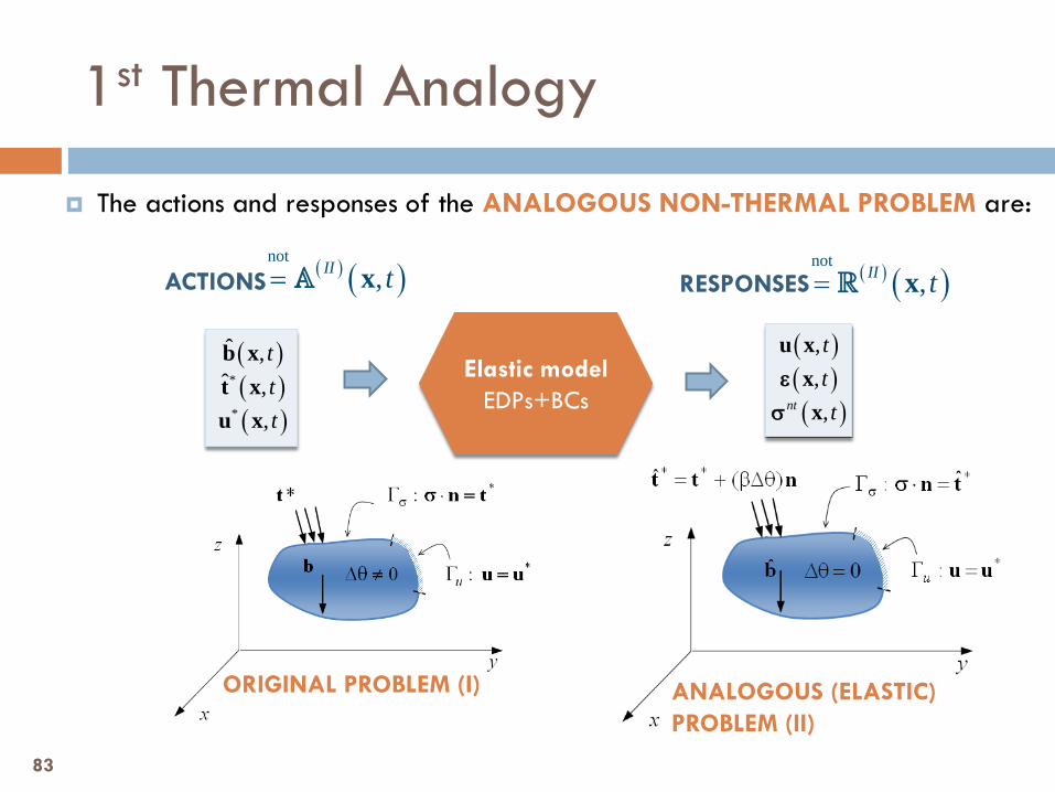
The actions and responses of the ANALOGOUS NON-THERMAL PROBLEM are:
( )( )( )
*
*
ˆ ,ˆ ,
,
ttt
b xt xu x
( )( )( )
,,,nt
ttt
u xxx
εσ
( ) ( )not
,II t= xAACTIONS ( ) ( )not
,II t= xRRESPONSES
Elastic model EDPs+BCs
ANALOGOUS (ELASTIC) PROBLEM (II)
ORIGINAL PROBLEM (I)
83

Responses are proven to be the solution of a thermoelastic problem under actions
If the actions and responses of the original and analogous problems are compared:
1st Thermal Analogy
( ) ( ) ( )( , ) ( , )def
I II III
nt nt
t tβ θ
− = − = = = − − ∆
u u 0 0x x 0 0R R Rε ε
σ σ σ σ 1
RESPONSES
ACTIONS ( ) ( )
( )
( )
( )0
* * * *
1ˆ ˆ
( , ) ( , ) ˆ ˆ
0
defI II IIIt t
β θρ
β θθ θ θ
∗ ∗
∆ − − = − = = =
− − ∆ ∆ ∆ ∆
b b b bu u 0 0x xt t t t n
A A A
∇
t= −σ
≡ b
*≡ t
84

( )t β θ
=== − = − ∆
u 00ε
σ σ 1
1st Thermal Analogy
ANALOGOUS ELASTIC
PROBLEM (II)
THERMOELASTIC ORIGINAL
PROBLEM (I)
THERMOELASTIC (TRIVIAL)
PROBLEM (III)
( )( )( )( )
*
*
,,,
,
ttt
tθ∆
b xt xu x
x
( )( )( )
,,,
ttt
u xxx
εσ
( ) ( ),I txA
( ) ( ),I txR
( ) ( ),II txA
( ) ( ),II txR
( ) ( ),III txA
( ) ( ),III txR
( ) ( )
( ) ( )( )
0* *
*
1ˆ ,
ˆ ,,0
t
tt
β θρ
β θ
θ
= − ∆
= + ∆
∆ =
b x b
t x t nu x
∇
( )( )
( )
,,
,nt
tt
t
u xx
xεσ
( )
( )
( )
0
*
1
, t
β θρ
β θ
θ
∗
= ∆
= − ∆=
∆
b
t nu 0
x
∇
86

2nd Thermal Analogy
The governing equations of the quasi-static isotropic linear thermoelastic problem are:
( ) ( )0, ,t tρ⋅ + =x b x 0∇ σ
( ) ( )-1, ,t t α θ= + ∆x : xCε σ 1
( ) ( ) ( )1, ,2
St t= = ⊗ + ⊗x u x u uε ∇ ∇ ∇
Equilibrium Equation
Inverse Constitutive Equation
Geometric Equation
*
*
:
:u
σ
Γ =
Γ = ⋅
u ut nσ Boundary Conditions in Space
87

2nd Thermal Analogy
The actions and responses of the problem are:
( )( )( )( )
*
*
,,,
,
ttt
tθ∆
b xt x
u x
x
( )( )( )
,,,
ttt
u xxx
εσ
( ) ( )not
,I t= xAACTIONS ( ) ( )not
,I t= xRRESPONSES
Elastic model EDPs+BCs
REMARK is known a priori, i.e., it is independent of the mechanical response. This is an uncoupled thermoelastic problem.
( ), tθ∆ x
88

If the thermal strain field is integrable, there exists a field of thermal
displacements, , which satisfies:
Then, the total displacement field is decomposed by defining:
2nd Thermal Analogy
( ),t tu x
( ) ( ) ( )
( )
1,2
1 , 1,2,32
t S t t t
ttjit
ij ijj i
t
uu i jx x
α θ
ε α θ δ
= ∆ = = ⊗ + ⊗
∂∂= ∆ = + ∈ ∂ ∂
x u u uε ∇ ∇ ∇1
The assumption is made that and are such that the thermal strain field is integrable (satisfies the compatibility equations).
( , )tθ∆ x ( )α x
( , ) ( , ) ( , )def
nt tt t t= −u x u x u x
REMARK The solution is determined except for a rigid body motion characterized by a rotation tensor and a displacement vector . The family of admissible solutions is . This movement can be arbitrarily chosen (at convenience).
( ) ( ) *, ,t t t ∗= + ⋅ +u x u x x c Ω
( ),t tu x∗Ω *c
nt t= +u u u89
t α θ= ∆ε 1

2nd Thermal Analogy
To solve the problem following the methods used in linear elastic problems, the thermal terms must be removed.
The strain tensor and the displacement vector splits, and are replaced into the governing equations: Geometric equations:
Boundary equations:
nt t= +ε ε ε nt t= +u u u
t
t
( )S S nt t S nt S t S nt
ntt
nt
= = + = + = +
= +
u u u u u uε ∇ ∇ ∇ ∇ ∇ ε
ε ε εεε
*nt t+ =u u u
nt S nt= uε ∇
* *: nt tuΓ = = −u u u u u
*
nt t== +
u uu u u
90
2nd Thermal Analogy
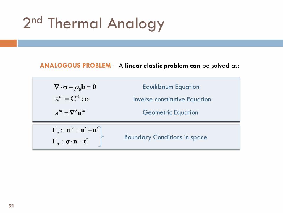
ANALOGOUS PROBLEM – A linear elastic problem can be solved as:
0ρ⋅ + =b 0∇ σ-1nt = :Cε σ
nt S nt= uε ∇
Equilibrium Equation
Inverse constitutive Equation
Geometric Equation
*
*
:
:
nt tu
σ
Γ = −
Γ ⋅ =
u u un tσ
Boundary Conditions in space
91

The actions and responses of the ANALOGOUS PROBLEM are:
( )( )
( ) ( )
*
*
,,
, ,nt t
tt
t t= −
b xt xu u x u x
2nd Thermal Analogy
( )( )
( )
,,
,
nt
nt
tt
t
u xx
xεσ
( ) ( )not
,II t= xAACTIONS ( ) ( )not
,II t= xRRESPONSES
Elastic model EDPs+BCs
ANALOGOUS PROBLEM (II) ORIGINAL PROBLEM (I)
92

If the actions and responses of the original and analogous problems are compared:
2nd Thermal Analogy
( ) ( ) ( )( , ) ( , )
nt t t
defI II IIInt tt t α θ
− = − = = ∆ =
u u u ux x
0 0R R Rε ε ε
σ σ1
RESPONSES
ACTIONS ( ) ( ) ( )
* *( , ) ( , )
0
t t defI II IIIt t
θ θ
∗ ∗
− − = − = = ∆ ∆
b b 0u u u u
x xt t 0
A A A
Responses are proven to be the solution of a thermo-elastic problem under actions
93
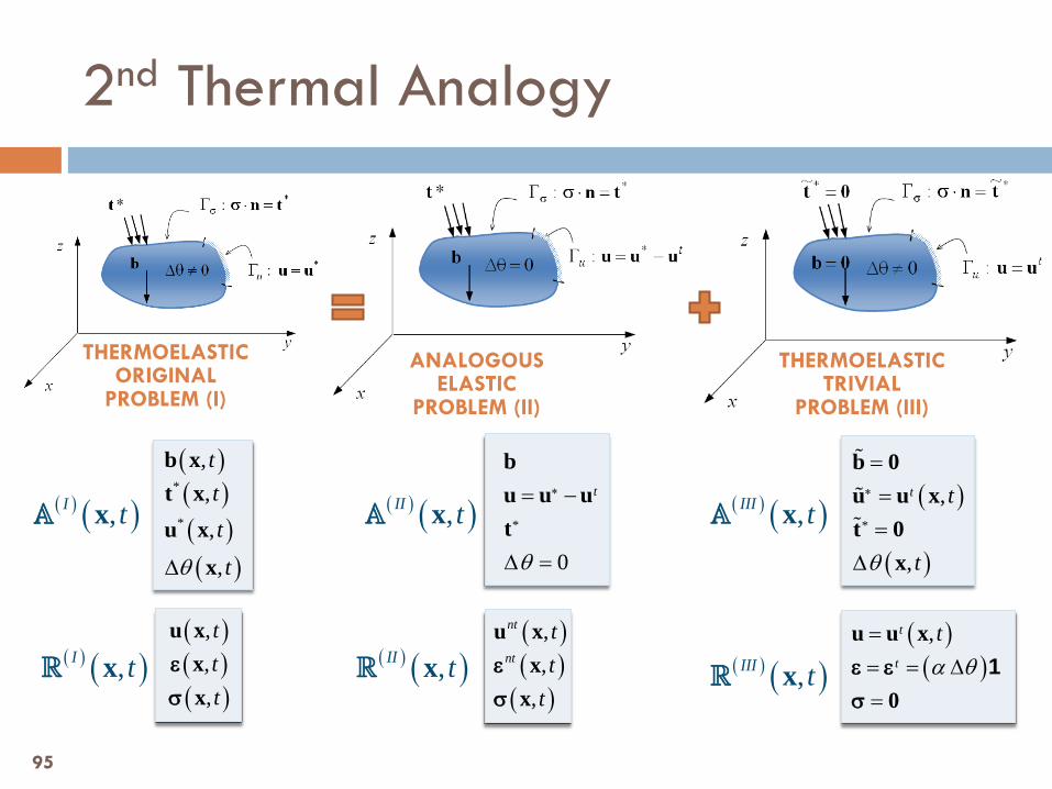
( )( ),t
t
tα θ
== = ∆=
u u x
0ε εσ
1
2nd Thermal Analogy
ANALOGOUS ELASTIC
PROBLEM (II)
THERMOELASTIC ORIGINAL
PROBLEM (I)
THERMOELASTIC TRIVIAL
PROBLEM (III)
( )( )( )( )
*
*
,,,
,
ttt
tθ∆
b xt xu x
x
( )( )( )
,,,
ttt
u xxx
εσ
( ) ( ),I txA
( ) ( ),I txR
( ) ( ),II txA
( ) ( ),II txR
( ) ( ),III txA
( ) ( ),III txR( )( )
( )
,,
,
nt
nt
tt
t
u xx
xεσ
( )
( )*
,
,
t t
tθ
∗
===
∆
b 0u u xt 0
x
*
0
t
θ
∗= −
∆ =
bu u ut
95

2nd Analogy in structural analysis
:
tx x
tx x
tu x x x
u u x
u u
α θ
ε ε α θ
α θ=
= = ∆
= = ∆
Γ = = ∆
*
0
:
ntx x
ntx x
tu x x x x
u u
u u u
ε ε
α θ=
=
=
Γ = − = − ∆
96

Although the 2nd analogy is more commonly used , the 1st analogy requires less corrections.
The 2nd analogy can only be applied if the thermal strain field is integrable. It is also recommended that the integration be simple.
The particular case Homogeneous material: Lineal thermal increment:
is of special interest because the thermal strains are: and trivially satisfy the compatibility conditions (involving second
order derivatives).
Thermal Analogies
( ) .x constα α= =ax by cz dθ∆ = + + +
t θ= α ∆ =1ε linear polinomial
97

In the particular case Homogeneous material: Constant thermal increment:
the integration of the strain field has a trivial solution because the thermal strains are constant , therefore:
The thermal displacement is:
Thermal Analogies
( ) .x constα α= =( ) .x constθ θ∆ = = ∆
.t constθ α = ∆ε =1
( ),t t α θ ∗ ∗= ∆ + ⋅ +u x x x cΩ
rigid body motion (can be chosen arbitrarily:
at convenience)
( ),t t α θ= ∆u x x ( )1t α θ α θ+ = + ∆ = + ∆x u x x x
HOMOTHECY (free thermal expansion)
98

99
Ch.6. Linear Elasticity
6.7 Superposition Principle

Linear Thermoelastic Problem
The governing eqns. of the isotropic linear thermoelastic problem are:
( ) ( )0, ,t tρ⋅ + =x b x 0∇ σ
( ) ( ), ,t t β θ= − ∆x : xCσ ε 1
( ) ( ) ( )1, ,2
St t= = ⊗ + ⊗x u x u uε ∇ ∇ ∇
Equilibrium Equation
Constitutive Equation
Geometric Equation
*
*
:
:u
σ
Γ =
Γ = ⋅
u ut nσ Boundary Conditions in space
( )( ) 0
,0
,0
=
=
u x 0
u x v
Initial Conditions
100

Linear Thermoelastic Problem
Consider two possible systems of actions:
and their responses :
( ) ( )( ) ( )( ) ( )
( ) ( )( ) ( )
1
1*
1*
1
10
,
,
,
,
t
t
t
tθ∆
b x
t x
u x
x
v x
( ) ( )( ) ( )( ) ( )
1
1
1
,
,
,
t
t
t
u x
x
x
ε
σ
( ) ( )1 , t ≡xA
( ) ( )1 , t ≡xR
( ) ( )( ) ( )( ) ( )
( ) ( )( ) ( )
2
2*
2*
2
20
,
,
,
,
t
t
t
tθ∆
b x
t x
u x
x
v x
( ) ( )2 , t ≡xA
( ) ( )( ) ( )( ) ( )
2
2
2
,
,
,
t
t
t
u x
x
x
ε
σ
( ) ( )2 , t ≡xR
101

The solution to the system of actions where and are two given scalar values, is .
This can be proven by simple substitution of the linear combination of actions and responses into the governing equations and boundary conditions.
When dealing with non-linear problems (plasticity, finite deformations, etc), this principle is no longer valid.
The response to the lineal thermoelastic problem caused by two or more groups of actions is the lineal combination of the responses caused by each action individually.
Superposition Principle
( ) ( ) ( ) ( ) ( )3 1 1 2 2λ λ= +A A A( ) ( ) ( ) ( ) ( )3 1 1 2 2λ λ= +R R R( )1λ ( )2λ
102

103
Ch.6. Linear Elasticity
6.8 Hooke’s Law in Voigt Notation

Taking into account the symmetry of the stress and strain tensors, these can be written in vector form:
Stress and Strain Vectors
x xy xz
xy y yz
xz yz z
σ τ ττ σ ττ τ σ
≡
σ
.
1 12 2
1 12 21 12 2
x xy xz
x xy xz not
xy y yz xy y yz
xz yz z
xz yz z
ε γ γε ε εε ε ε γ ε γε ε ε
γ γ ε
= =
ε
6
x
y
defz
xy
xz
yz
σσστττ
= ∈
Rσ
6
x
y
defz
xy
xz
yz
εεεγγγ
= ∈
Rε
REMARK The double contraction is transformed into the scalar (dot) product :
( )σ : ε
( )⋅σ ε
= ⋅σ : ε σ ε ij ij i iσ ε σ ε=2nd order tensors
vectors
VOIGT NOTATION
104
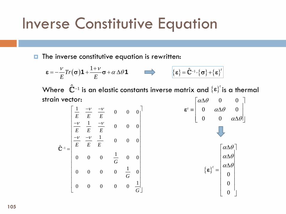
The inverse constitutive equation is rewritten:
Where is an elastic constants inverse matrix and is a thermal
strain vector:
Inverse Constitutive Equation
( ) 1TrE Eν ν α θ+
= − + + ∆ε σ σ1 1 1ˆ t−= ⋅ +Cε σ ε
1
1 0 0 0
1 0 0 0
1 0 0 0ˆ
10 0 0 0 0
10 0 0 0 0
10 0 0 0 0
E E E
E E E
E E E
G
G
G
ν ν
ν ν
ν ν
−
− −
− − − −
=
C
1ˆ −C tε
0 00 00 0
t
α θα θ
α θ
∆ ≡ ∆ ∆
ε
000
t
α θα θα θ
∆ ∆ ∆
=
ε
105
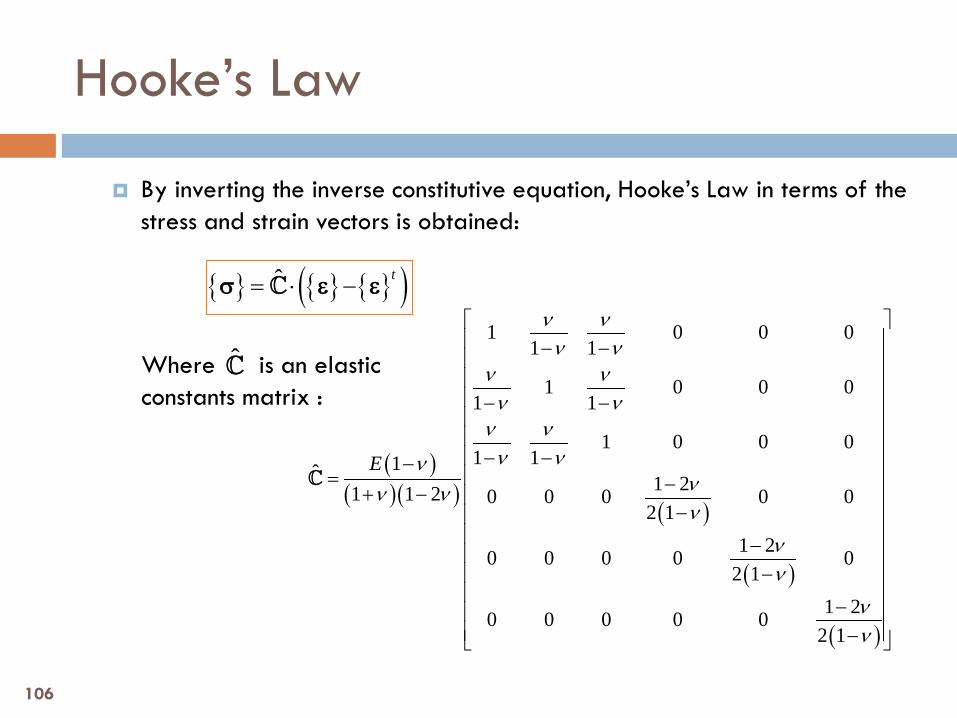
By inverting the inverse constitutive equation, Hooke’s Law in terms of the stress and strain vectors is obtained:
Where is an elastic constants matrix :
Hooke’s Law
C
( )ˆ t= ⋅ −Cσ ε ε
( )( )( )
( )
( )
( )
1 0 0 01 1
1 0 0 01 1
1 0 0 01 11ˆ 1 21 1 2 0 0 0 0 0
2 11 20 0 0 0 0
2 11 20 0 0 0 0
2 1
E
ν νν ν
ν νν ν
ν νν νν
νν νν
νν
νν
− − − − − −− = −+ −
− −
−
− −
C
106


