Chalmers Publication Library Fast Analysis of Periodic Antennas and Metamaterial-Based Waveguides This document has been downloaded from Chalmers Publication Library (CPL). It is the author´s version of a work that was accepted for publication in: Computational Electromagnetics – Recent Advances and Engineering Applications Citation for the published paper: Maaskant, R. (2014) "Fast Analysis of Periodic Antennas and Metamaterial-Based Waveguides". Computational Electromagnetics – Recent Advances and Engineering Applications pp. 75-109. http://dx.doi.org/10.1007/978-1-4614-4382-7_3 Downloaded from: http://publications.lib.chalmers.se/publication/194108 Notice: Changes introduced as a result of publishing processes such as copy-editing and formatting may not be reflected in this document. For a definitive version of this work, please refer to the published source. Please note that access to the published version might require a subscription. Chalmers Publication Library (CPL) offers the possibility of retrieving research publications produced at Chalmers University of Technology. It covers all types of publications: articles, dissertations, licentiate theses, masters theses, conference papers, reports etc. Since 2006 it is the official tool for Chalmers official publication statistics. To ensure that Chalmers research results are disseminated as widely as possible, an Open Access Policy has been adopted. The CPL service is administrated and maintained by Chalmers Library. (article starts on next page)
Transcript
Chalmers Publication Library
Fast Analysis of Periodic Antennas and Metamaterial-Based Waveguides
This document has been downloaded from Chalmers Publication Library (CPL). It is the author´s
version of a work that was accepted for publication in:
Computational Electromagnetics – Recent Advances and Engineering Applications
Citation for the published paper:Maaskant, R. (2014) "Fast Analysis of Periodic Antennas and Metamaterial-BasedWaveguides". Computational Electromagnetics – Recent Advances and EngineeringApplications pp. 75-109.
Notice: Changes introduced as a result of publishing processes such as copy-editing and
formatting may not be reflected in this document. For a definitive version of this work, please refer
to the published source. Please note that access to the published version might require a
subscription.
Chalmers Publication Library (CPL) offers the possibility of retrieving research publications produced at ChalmersUniversity of Technology. It covers all types of publications: articles, dissertations, licentiate theses, masters theses,conference papers, reports etc. Since 2006 it is the official tool for Chalmers official publication statistics. To ensure thatChalmers research results are disseminated as widely as possible, an Open Access Policy has been adopted.The CPL service is administrated and maintained by Chalmers Library.
Abstract A tailored version of the Characteristic Basis Function Method(CBFM) is presented as a matrix compression technique for the method-of-moments (MoM) to rapidly compute the impedance, radiation, and propaga-tion characteristics of large periodic structures, including antenna arrays andmetamaterial-based waveguides. The compression is achieved by employingphysics-based Characteristic Basis Functions (CBFs), which are generatednumerically and in a time-efficient manner by exploiting array symmetries.The supports of these CBFs partially overlap between electrically intercon-nected array elements to preserve the continuity of the surface current acrosscommon boundaries. The translation symmetry is also exploited to expedite
R. MaaskantChalmers University of Technology S-41296 Gothenburg, Sweden, e-mail: rob.
the meshing process of the structure, to construct the reduced matrix equa-tion, and to rapidly compute the antenna radiation patterns. The AdaptiveCross Approximation (ACA) algorithm is applied to reduce the matrix fill-time even further. The numerical examples demonstrate high accuracy andexcellent memory compressing capabilities of the considered method. Amongthe problems, we consider a very large array of nested subarray antennas em-ploying more than 1E6 low-level basis functions, which is solved directly, in-core, through a multilevel CBFM approach, and we analyze a metamaterial-based gap waveguide through a CBFM-enhanced MoM approach employingthe parallel-plate Green’s function.
1 Introduction1
Recent advances in computational electromagnetics (CEM) have enabled usto analyze large real-world antenna and scattering problems that were beyondour reach only a few years ago. In this chapter, we will provide only a limitedoverview of the literature that is closely related to the problem at hand,namely, fast analysis of large finite periodic structures, including antennaarrays and novel metamaterial-based waveguide structures analyzed throughthe Method-of-Moments (MoM, [14]).
Regarding the numerical analysis of finite periodic structures, asymptoticinfinite-array approaches with corrections for the edge truncation effects havebeen developed, which are effective when the edge behavior of an array is lo-cal, and almost independent of the array size. This is true for very large arrayswhere the center elements behave as infinite-array elements. One can thensolve for the fringe current describing the difference between the finite- andthe associated infinite-array current [33]. The advantage is that the fringecurrent can be expanded by using relatively few basis functions, derived froma diffraction analysis of canonical structures, whose use requires the solutionof only a moderately sized matrix equation. Other infinite-array-based tech-niques that expedite the finite array analysis can be found in [6, 8, 39, 44].Infinite array approaches are particularly efficient if both the structure andfields are (nearly) periodic; otherwise, the method may not be the preferredchoice. In fact, for moderate-sized arrays, and for those that require a highdegree of flexibility in terms of array lattice geometry and element shape, itis preferable to use methods that are based on analyzing finite-size arrays.
One can employ subsectional basis functions of higher-order polynomialsto reduce the size of the MoM matrix equation [11]; moreover, by employingmacro basis functions an even greater reduction in the number of unknownscan be achieved. Since macro-domain functions can be constructed as fixedcombinations of subsectional functions, these macro functions can conform to
1 This chapter is largely based upon Maaskant’s PhD dissertation [22].
Fast Analysis of Periodic Antennas and Metamaterial-Based Waveguides 3
arbitrarily shaped geometries. An additional advantage of using these macrobasis functions is that existing codes can be reused with only minor modifica-tions. These types of macro functions are sometimes referred to as aggregatedbasis functions, and have been applied to arrays of disconnected patch an-tennas in [47] and [15].
The expansion wave concept is also a method which reduces the number ofunknowns without compromising the solution accuracy or geometrical flex-ibility of the low-level basis functions. It decomposes both the incident andscattered fields to and from an isolated array element in terms of only a fewexpansion functions [46]. This concept of reducing the matrix equation anddecomposing the problem into smaller problems has been widely exploitedin recently developed iterative-free methods for large-scale problems. For in-stance, the Characteristic Basis Function Method (CBFM) [24,32,34,43,49],which has been successfully applied to a large class of scattering and ra-diation problems, the Synthetic-Functions Approach (SFX) [29], [31], theSub-Entire-Domain Basis Function Method (SED) [21], the eigencurrent ap-proach [2], which has recently been combined with the Linear Embeddingvia Green’s Operators approach (LEGO, [19]), and a subdomain multilevelapproach [41]. The objectives of these methods are similar, namely to re-duce the matrix equation by employing physics-based macro basis (and test)functions for the electric and/or magnetic surface currents.
In this chapter, we tailor the CBFM for the fast analysis of large periodicstructures. We propose a dedicated array meshing method which exploitsthe array translation symmetry and preserves the quasi-Toeplitz symmetryin the reduced MoM matrix. Special attention is devoted to the problem ofthe efficient generation of a representative set of Characteristic Basis Func-tions (CBFs), and this is only done for a few unique array elements. Also,since the array elements may be electrically interconnected to one another,a post-windowing technique is developed to shape the initially generatedCBFs in order to guarantee a piecewise continuous current flow at the in-terconnections by letting the CBFs partially overlap. This is an alternativemethod to [29], where one employs an additional independent set of “connec-tion” basis functions to ensure the electrical connectivity between adjacentantenna elements. Hence, the herein presented overlapping domain decom-position method (DDM) requires less unknowns and therefore enables us tosolve larger problems, although the method in [29] may provide a bettercontinuity of the current in the interconnection regions.
We point out that the savings realized in CBFM, in terms of both memoryand computation time, are significant; the solution time (for direct solvers)scales as O(N3), where N now becomes a relatively small number associ-ated with the total number of CBFs. The proportionality constant, however,slightly increases because of the additional time that is required to generateCBFs. The construction time of the reduced matrix scales as O(N2), whereN still represents the relatively large number of subsectional basis functionsmaking up the CBFs, so that the fill-time of the reduced matrix governs
the total execution time. A number of hybrid methods have been proposedto reduce the matrix-fill time. For instance, in [40] the reaction integral be-tween the macro basis and testing functions is computed using a suitableapproximation. A generalization of this approach has led to the introductionof the Fast Multipole Method (FMM) for the rapid computation of thesereactions [7], [11]. Alternatively, the Adaptive Integral Method (AIM) hasalso been applied to compute these reduced matrix entries efficiently [48], [3].In the present chapter we generate the reduced matrix in a time-efficientmanner by hybridizing the CBFM with the Adaptive Cross Approximation(ACA) algorithm. The ACA algorithm was originally developed for the rapidconstruction of the rank-deficient off-diagonal MoM matrix blocks [1,18,50];however, it will be shown that the algorithm is also suited to compute the off-diagonal MoM blocks of the CBF-reduced matrix in a time-efficient manner.The ACA algorithm is purely algebraic in nature, kernel independent andrelatively easy to implement. Furthermore, the algorithm does not require apriori knowledge of each MoM submatrix.
The above-described mathematical framework is supplemented with amethodology to rapidly compute the radiation and port impedance char-acteristics, and the multilevel CBFM is described as a generalization of themonolevel CBFM afterwards.
The accuracy of the method is assessed for a 7×1 array of Tapered Slot An-tennas (TSAs). Their analyses constitutes a challenging numerical problem,since the outer edges of the TSA fins are (entirely) connected to the adjacentelements as a result of which the analysis of the entire array problem cannotbe localized to the analysis of a single isolated TSA element. Following this,the numerical results are presented on the CBFM–ACA hybridization. Thisis followed up by the extremely large problem of solving large antenna arraysof nested disjoint subarrays, whose solution is found through the multilevelCBFM. Finally, we consider a low-loss low-cost novel class of waveguides: theso-called gap waveguides. Gap waveguides are metameterial-based waveg-uides employing periodic textures of small metallic objects to emulate anartificial magnetic conductor, thereby exhibiting superior propagation char-acteristics to the more conventional waveguides. It is shown that the CBFMcan handle these fine-feature structures with relative ease, even if the problemgrows very large.
2 The Characteristic Basis Function Method (CBFM)
For the sake of completeness, we briefly review the CBFM in this section,though the method has also been discussed in a number of other chapters inthis book for a variety of other problems for different applications, e.g., RCScomputation and analysis of microwave integrated circuits.
In algebraic terms, the objective of CBFM is to solve the large system oflinear equations
ZI = V (1)
for the unknown coefficient vector I in an iteration-free and time-efficientmanner. The complex symmetric matrix Z is of size N×N and assumed largeenough to pose a severe computational burden on the memory storage andmatrix fill times, let alone on the numerical solution of (1). This limitationcan be overcome by CBFM, which is capable of solving the system directly formultiple right-hand-sides (MRHS) and in-core for N upwards of one million,or even larger, depending upon the computational platform.
The degrees of freedom (DoFs) of the solution vector I in (1) isN . However,the solution vector tends to lie in a much smaller subspace for most practicalEM problems that are solved through the method of moments (MoM) em-ploying a fine discretization scheme. For instance, for a transmitting dipoleantenna, the solution vector I – representing the current in terms of N subsec-tional basis functions – most likely resembles a cosine-type of function. Theactual dipole current can therefore be represented rather accurately througha very low number of linearly independent solution vectors, or macro basisfunctions – called Characteristic Basis Functions (CBFs) – resembling thecos-type of functions. Hence, the key feature of CBFM is to reduce the DoFsof I by two-to-three orders through a physics-based expansion such as:
I =
Q∑q=1
ICBFq JCBF
q (2)
where JCBFq are the Q CBFs (Q N), and ICBF
q are the correspondingCBF expansion coefficients. Substituting (2) in (1), yields
Q∑q=1
ICBFq ZJCBF
q = V (3)
after which the error R can be defined as R =∑Qq=1 I
CBFq ZJCBF
q −V. Weight-
ing this error to zero using Q testing vectors JCBFp Qp=1 that are identical to
where the symmetric dot-product 〈a,b〉 = aTb, and where the superscriptT denotes the transposition operator. Eq. (4) represents a reduced matrixequation ZredICBF = Vred, where Zred is of size Q×Q, whose matrix elementZredpq = 〈JCBF
p ,ZJCBFq 〉, and where the pth element of the N × 1 RHS vector
Vredp = 〈JCBF
p ,V〉.Two major questions remain: (i) how to generate a representative set of
CBFs (to be discussed in Sec. 2.2), and; (ii) how to rapidly generate thereduced matrix equation (4). Indeed, Eq. (4) contains computationally ex-pensive matrix-vector products, and also requires constructing the originalmoment matrix Z, both of which are both time-consuming tasks.
We can alleviate the burden of the matrix-vector multiplications as fol-lows. Consider the example of a 7 × 1 singly-polarized TSA array in Fig. 1.The entire surface S supporting the surface current is triangulated, after
Jp
S
Sq
Jq
Sp
Zredpq = 〈Jp,ZpqJq〉
Fig. 1 Reduced matrix element Zredpq ; the dot product between the (observation)
CBF Jp and the excitation vector ZpqJq due to the (source) CBF Jq.
which pairs of triangles form N Rao-Wilton-Glisson (RWG) basis func-tions for modeling the current [35]. To rapidly compute the matrix elementZredpq = 〈JCBF
p ,ZJCBFq 〉 in (4), we note from Fig. 1 that if the supports of the
CBFs are local – in this case about the size of a single antenna element – theCBFs will contain many zeros. Indeed, when squeezing out the zero entries,i.e., JCBF
p 7→ Jp and JCBFq 7→ Jq, effectively only the matrix block Zpq of Z rep-
resenting the interactions between the group pair of RWGs on the subdomainsSp and Sq need be computed, and we can write Zred
pq = 〈Jp,ZpqJq〉. Similarly,
the zero entries in V on the RHS can be discarded, so that Vredq = 〈Jp,Vp〉
in (4), where Vp is a subset of V pertaining to the local support Sp.The final reduced matrix equation can be written as
Fast Analysis of Periodic Antennas and Metamaterial-Based Waveguides 7〈J1,Z11J1〉 〈J1,Z12J2〉 · · · 〈J1,Z1LJL〉〈J2,Z21J1〉 〈J2,Z22J2〉 · · · 〈J2,Z2LJL〉
......
. . ....
〈JL,ZL1J1〉 〈JL,ZL2J2〉 · · · 〈JL,ZLLJL〉
ICBF1
ICBF2
...
ICBFL
=
〈J1,V1〉〈J2,V2〉
...
〈JL,VL〉
(5)
where we now have assumed that the subdomain Sp can generally support
more than one, say Qp, CBFs, so that the Qp columns in the matrix ICBFp are
the expansion coefficient vectors for the CBFs on the pth subdomain. Thetotal number of employed CBFs is therefore the sum of all the CBFs persubdomain, thus Q =
∑Lp=1Qp, where L is the total number of subdomains.
We observe that the CBFM can be thought of as a domain decomposi-tion method (DDM), since the CBFs have a local support and need to begenerated only for a smaller subproblem as detailed in the next section.
2.2 Generation of CBFs
Note that the supports of the CBFs in Fig. 1 slightly extend beyond the size ofa single TSA element, so that the subdomains partially overlap. Such partialoverlapping preserves the continuity of the surface current across the commonboundaries between interconnected TSAs when CBFs are superimposed toform the spurious-free solution for I in (1). This specific implementation isreferred to as an overlapping DDM, although non-overlapping DDMs can beimplemented as well that employ additional subsectional basis functions inorder to mitigate the interface glitch effects [30].
While [24] presents a generic technique to generate the CBFs for arraysof electrically interconnected antenna elements, only the most widely usedversion of this technique will be considered hereafter. The procedure for gen-erating the CBFs is explained in four stages below for the example depictedin Fig. 2.
Step I: Mesh generationOnly a single TSA element is triangulated and replicated at various elementpositions throughout the array lattice by means of geometrical translations.While rapidly generating the entirely meshed structure, the partitioning ofRWGs is kept identical for each array element and the polarity of the RWGsthat electrically interconnect the antenna elements is chosen consistently,and such that the entirely meshed array facilitates a one-to-one mapping ofpartially overlapping CBFs. This mapping of CBFs has been visualized inthe transition from Step III to Step IV (see also Sec. 3.1 for more details).
Step II Generation of primary CBFsThree subarrays are extracted from the entirely meshed array to generatethe CBFs, i.e., two corner elements and one central element along with theirelectrically interconnected adjacent element(s). Since we are here interested
Fig. 2 Step I: fully meshed 7x1 TSA array; Step II: extraction of 3 subarrays forgenerating the CBFs; Step III: truncation of the subarray induced currents to formthe CBFs; Step IV: mapping of CBFs onto the fully meshed array, constructing thereduced matrix equation (5), and the final synthesized surface current solution forbroadside scan.
in computing the antenna impedance matrix and radiation patterns, we con-sider the problem on transmit, so that the primary CBFs are also generatedon transmit to achieve an accurate representation of the current. These aregenerated by exciting each accessible port of the three subarrays sequen-tially. As a result, the number of primary generated CBFs equals the numberof accessible ports for each subarray.
More specifically, suppose that for one of the subarrays in Step II, thecurrent on a subarray is expanded into Nsub RWG basis functions, then thesubarray currents are found by solving a small matrix equation for the MRHSN ×K column-augmented excitation matrix Vsub, i.e.,
Fast Analysis of Periodic Antennas and Metamaterial-Based Waveguides 9
Isub = Z−1subVsub (6)
where Zsub is the moment matrix of the corresponding subarray RWGs, andthe K columns of the matrix Isub are the induced currents when exciting theports of the subarrays. As a result, two primary CBFs are generated on theouter two subarrays, while three CBFs are generated on the inner subarray.
It should be pointed out that, when analyzing the entire structure as ascattering problem, one is typically interested in its response to a series ofplane waves incident from various directions. Hence, it is natural to also leta plane-wave spectrum (PWS) be incident on each subarray for generatingthe initial set of CBFs. Although this is an obvious choice for scatteringproblems, antenna array problems have been analyzed successfully using thePWS-generated CBFs as well, both for the receive and transmit cases [23].
Step IIIa Truncation and Post-Windowing of CBFsNext, we apply a trapezoidal windowing function Λ to each of the sets ofCBFs that were generated for the subarrays in Fig. 2, Step II, in order toarrive at Step III, where the spurious edge-singular currents arising fromsubarray truncation effects have been eliminated [24]. In particular, we willemploy a pulse windowing function to reduce the support of each CBF tothe size of one antenna element only, while retaining possible “connection”RWGs. Note the one-cell overlap in Step III at connecting boundaries whereindeed no edge truncation effects are visible.
For each subarray, the final windowed set of CBFs Jsub (Step III, Fig. 2)is thus computed as
Jsub = ΛIsub = ΛZ−1subVsub (7)
where the diagonal matrix Λ post-multiplies the RWGs in the initial set ofCBFs Isub either by 0, 1/2, or 1, depending upon whether they are in theexternal, overlap, or internal region of the resulting truncated subdomain,respectively. Note that the “connection” RWGs in the overlap region arecolored bluish as a result of weighting these RWGs by 1/2, while the zeros inJsub are discarded to truncate the support. The RWGs are weighted by 1/2to make sure that, when adjacent CBFs are superimposed, the sum of theweights of each pair of overlapping RWGs amounts to unity again. If threeconductors are connected, one has to multiply by 1/3, and so on.
Step IIIb Reducing the number of CBFs by using the SVDTo obtain a well-conditioned reduced moment matrix in (5), it is necessarythat the CBFs be linearly independent, which can be assured through aSingular Value Decomposition (SVD) operation as this renders the CBFsorthogonal.
Let the matrix Jq be of size Nq ×Kq, where Nq and Kq denote the totalnumber of RWGs and the number of initially generated CBFs on the qthsubdomain, respectively. Upon invoking the SVD, Jq is decomposed as
where U is an Nq×Kq matrix with orthonormal columns/CBFs [45, p. 27]; Qis a Kq×Kq unitary matrix; and, D is a Kq×Kq diagonal matrix of the formdiag(σ1, σ2, . . . , σKq
). The non-negative real-valued diagonal entries of D canbe required to be ordered as σ1 ≤ σ2 ≤ . . . ≤ σKq
and are the singular valuesof Jq. The presence of singular values of zero, or near-zero, indicates thatthe matrix is singular or ill-conditioned. Therefore, to improve this conditionnumber, a thresholding procedure is used on the normalized singular values
Rn =σnσmax
n = 1, 2, . . . ,Kq. (9)
Each of these normalized quantities is compared to an appropriate threshold,and the corresponding singular value is set to zero if this level is smallerthan the specified threshold. Suppose this happens for n > Nσ, then the firstNσ left singular vectors of U forms the orthonormal set of CBFs that areretained.
Step IIIc Generation of Secondary CBFsThe accuracy of the final solution for the current can be increased further byaccounting for the mutually coupled subdomains in a more detailed mannerthrough employing additional higher-order CBFs. Then, the primary CBFsJq, which are supported by the qth subdomain are, in turn, used as distantcurrent sources to the subarrays shown in Step II (Fig. 2) to mimic possiblesurface currents on neighboring array elements that are located within acertain electrical distance from the subarray under excitation. Following (6),the currents Jsub on a subarray are then computed as
Isub = Z−1subVsub = Z−1subZsub,qJq (10)
where Zsub,q is the moment matrix block between the RWGs on the qth sourcedomain, which supports a set of primary source CBFs Jq, and the RWGs onthe subarray under excitation. Accordingly, the CBF support is truncatedby using (7), appended to the existing set of primary CBFs, and then wefollow this up with an SVD orthogonalization-thresholding procedure. If thecombined set of initially generated primary and secondary CBFs is sufficientlysmall, it is suffiecient to perform the SVD only once. However, a multi-stageSVD procedure has been found to be more efficient in most cases, also forscattering problems where the primary CBFs are typically generated by usinga PWS approach [10].
The total number of initially-generated secondary CBFs depends uponthe total number of distant subdomains that are considered within a certainradius from the subarray under excitation. To increase the number of CBFs,one can also generate tertiary CBFs from the primary and secondary ones.However, at some point the SVD prevents us from adding more CBFs that arenot sufficiently independent of the existing set of CBFs. Hence, convergence
Fast Analysis of Periodic Antennas and Metamaterial-Based Waveguides 11
of the solution depends upon the final solution accuracy desired, and this iscontrollable through the choice of the SVD threshold.
Step IV Mapping of CBFs and solving for the currentAfter retaining a relatively small set of CBFs for each truncated subdo-main (Step III, Fig. 2), the CBFs are mapped onto the various subdomainsthroughout the entire array (Step IV, Fig. 2). Afterwards, the reduced ma-trix equation in Eq. (5) is constructed and solved directly for MRHS withoutresorting to iterative techniques. The resulting surface current for the 7 × 1TSA array is shown in Fig. 2 for a broadside scan, when all the elements areexcited by a voltage source across the slotline section.
3 Fast Reduced Matrix Generation
3.1 Exploiting Array Translation Symmetry
The reduced moment matrix Zred in (5) can be constructed efficiently byexploiting the translation symmetry between CBFs. As an example, Fig. 3graphically exemplifies that the reduced matrix block Zred
pq equals Zredp+1;q+1,
because both blocks represent reactions between identical, though translated,set of CBFs. It follows that,
Zredpq = 〈Jp,ZpqJq〉 = 〈Jp+1,Zp+1;q+1Jq+1〉 = Zred
p+1;q+1 (11)
provided that both Sq and Sp [see Fig. 3(a)] support sets of CBFs that mapone-to-one onto the one-element translated subdomains Sq+1 and Sp+1 [seeFig. 3(b)], respectively, using the same translation vector. Hence, to fullyexploit translation symmetry, the periodic structure must be discretized ina specific manner to facilitate this CBF mapping and, hence, a consistenttriangulation and partitioning of the RWGs of all subdomains (and thusarray elements) is required as further clarified below.
The entire array mesh can be efficiently constructed from a few elementarymeshed array elements, called the base elements, see for instance the bowtieelement in Fig. 4 (Step I). The geometry of each base element is discretizedby a number of polygonal facets of which the outlines are described by aset of boundary nodes (black dots). Here, the bowtie base element comprisesof 3 polygonal surfaces, i.e., two triangular fins and one small port polygonconnecting the fins. Each planar polygonal facet is supplied by a non-uniformgrid of internal nodes and subsequently triangulated in a 2-D plane by usinga Delaunay meshing routine [4, 9]. The internal grid is distributed such thatthe elementary triangles are very nearly equilateral. Subsequently, nodes andtriangles are added along the boundaries to ensure that the triangulationswould be consistent with those of the electrically interconnected adjacentelements when these base elements are placed in the array environment. Next,
Fig. 3 Construction of identical reduced matrix blocks Zredpq and Zred
p+1;q+1.
triangulated base elements are equipped with the RWGs. Step I (Fig. 4)shows a possible RWG polarity distribution, visualized by vectors that jointhe common edges of each pair of triangles to form an RWG.
Step II illustrates a one-to-one replication of the discretized base elementat array element locations r1 . . . r5. Note that, at this stage, the RWGs en-suring the electrical connection between array elements have not yet beenestablished. This is accomplished in Step III, where the triangles along a con-nection line are separately equipped with RWGs and subsequently mapped(recursively) onto the various corresponding connection lines that remain tobe equipped with RWGs. For this purpose, we utilize the array symmetry asdetailed below. A pseudo Matlab code of the recursive-mapping algorithm isincluded in the appendix of [26]. Finally, a full meshing of the array geom-etry (Step IV) facilitates a one-to-one mapping of the CBFs, even thougheach supporting subdomain extends beyond the outer boundaries of an arrayelement, as shown in Fig. 3.
Next, the translation symmetry between identical pairs of CBFs can bedetermined. Following the generation of the boundary nodes for the array ina manner shown in Fig. 4, Step II, where we replicate the boundary nodes ofthe base antenna element(s) at their respective array positions, we can deter-mine which array elements are electrically interconnected. Furthermore, when
Fast Analysis of Periodic Antennas and Metamaterial-Based Waveguides 13
Fig. 4 Efficient and consistent meshing of the antenna array structure to fully exploittranslation symmetry.
using multiple base elements, such as in the case of dual-polarized arrays, onecan also keep track of the type of base element that is interconnected. Let theelement interconnection and the corresponding base element type be storedin two separate matrices. Then, for our example, using only one type of baseelement (the bowtie element in Fig. 4, Step I), we have:
1 2 0
2 1 3
3 2 4
4 3 5
5 4 0
and
1 1 0
1 1 1
1 1 1
1 1 1
1 1 0
(12)
where the first rows of the left- and right-hand matrices indicate that antennaelement 1 is connected to antenna element 2, and that they are both baseelements of type-1 (ignore the zero entries), and so forth.
Also, for each array element, one can determine the relative positions ofthe electrically interconnected elements surrounding it. Upon comparing thegroups of relative position vectors in conjunction with the corresponding
base element types (rows of second matrix), one can readily determine whichsubdomains (and therefore corresponding set of CBFs) are identical. For ourexample, subdomains 2, 3, 4; 1; and 5 form the 3 unique groups. Weneed to only generate one set of CBFs per unique subdomain, in this casefor subdomains 1, 5 and 3, where subdomain 3 is chosen from the first groupas the most central element. Elements 1, 5 and 3 are extracted from thefully meshed array, together with their neighboring array elements (withina specified radius), to form the resulting three subarrays that are used togenerate the CBFs. After windowing these CBFs, the CBFs supported bysubdomain 3 are mapped onto the subdomains 2, 3, and 4.
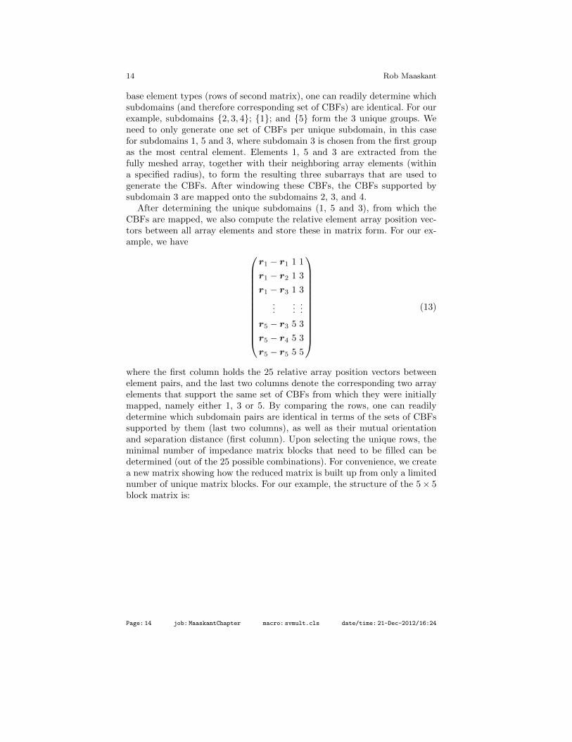
After determining the unique subdomains (1, 5 and 3), from which theCBFs are mapped, we also compute the relative element array position vec-tors between all array elements and store these in matrix form. For our ex-ample, we have
r1 − r1 1 1
r1 − r2 1 3
r1 − r3 1 3
......
...
r5 − r3 5 3
r5 − r4 5 3
r5 − r5 5 5
(13)
where the first column holds the 25 relative array position vectors betweenelement pairs, and the last two columns denote the corresponding two arrayelements that support the same set of CBFs from which they were initiallymapped, namely either 1, 3 or 5. By comparing the rows, one can readilydetermine which subdomain pairs are identical in terms of the sets of CBFssupported by them (last two columns), as well as their mutual orientationand separation distance (first column). Upon selecting the unique rows, theminimal number of impedance matrix blocks that need to be filled can bedetermined (out of the 25 possible combinations). For convenience, we createa new matrix showing how the reduced matrix is built up from only a limitednumber of unique matrix blocks. For our example, the structure of the 5× 5block matrix is:
Fast Analysis of Periodic Antennas and Metamaterial-Based Waveguides 15
Subdomain# 1 2 3 4 5
1
2
3
4
5
1 2 3 4 5
6 7 8 9
6 7 10
6 11
12
(14)
where 12 out of 25 non-redundant mutual impedance blocks have been identi-fied, since we also exploited reciprocity (only the upper triangular part of thematrix is required). Note that, for this example, the matrix entry 7 denotesthat the reactions between the CBFs supported by subdomains (antenna ele-ments) 2 and 3 are identical to the reactions between the CBFs supported bythe subdomains 3 and 4, as we can verify from Fig. 4. In conclusion, symmetrycan be exploited for arrays of electrically interconnected elements to reducethe complexity of the matrix-filling process. For the present example of aregular-spaced single-polarized antenna array (Fig. 4), it can be shown thatthe computational complexity becomes linear when the translation symmetryis exploited.
3.2 The Adaptive Cross Approximation (ACA)Algorithm
If we exploit the quasi-Toeplitz structure in Eq. (5), we would only need toconstruct relatively few of these matrix blocks and reduce the matrix fill-time. The matrix fill-time can be further reduced as explained below. It isinteresting to note that (5) suggests that a full matrix block Zpq has to bebuilt before its compressed version 〈Jp,ZpqJq〉 can be computed. Since Zpqis rank deficient, if this matrix block represents the interactions between adistant group pair of RWGs, we can write:
Zredpq = 〈Jp,ZpqJq〉 ≈ 〈Jp, ZpqJq〉 (15)
where Zpq is a low-rank decomposition of Zpq, factorized in terms of a fewrelatively small sub-matrices2.
The degree of rank deficiency of Zpq depends on the electrical distance thatseparates the observation and source groups p and q, as well as their sizesand mutual orientations [25]. The effective rank decreases for an increasinglylarger separation distance. For well-separated groups of RWGs, the voltageexcitation vector at the observation group p, produced by any source RWG,
2 Alternatively, in [48], each column of the matrix product ZpqJq is computed effi-ciently as an AIM matrix vector product.
can be expressed as a linear combination of the voltage vectors resulting fromonly a few of these source RWGs (source sampling). Likewise, the voltageexcitation vector at the observation group p produced by any source RWGcan be expressed as a linear combination of the voltage vectors of a fewof these observation RWGs (field sampling). Hence, a cross-approximationtechnique can be used to adaptively construct the subsets of relevant sourceand observation RWGs.
In this work, we employ the Adaptive Cross Approximation (ACA) al-gorithm [1, 18, 50], which is an adaptive and on-the-fly rank-revealing blockfactorization of the rank-deficient sub-matrices. The ACA algorithm is purelyalgebraic in nature, and can be used irrespectively of the nature of the kernelof the integral equation, or the the basis functions or type of integral equationformulation. This makes the ACA algorithm attractive for handling problemsinvolving arbitrary geometries and therefore suits the CBFM paradigm. Inaddition, the ACA algorithm only requires a partial knowledge of the orig-inal matrix and belongs to a large group of fast integral equation algebraicmethods (see [50], and references therein). It has been shown that for low-frequency EMC problems of moderate electrical size both the memory andCPU time requirements for the ACA algorithm scale as N4/3 logN [50].
The ACA algorithm approximates Zpq through the following block factor-ization
Zpq = UNp×rkp Vrk×Nq
q =
rk∑i=1
uNp×1i v
1×Nq
i (16)
where rk is a short-hand notation for rk(Zpq), which denotes the effective
rank of the matrix Zpq. Further, UNp×rkp is a column-augmented matrix of size
Np×rk, and Vrk×Nqq is a row-augmented matrix of size rk×Nq. The ith column
vector of U and the ith row vector of V are denoted by ui and vi, respectively.It is evident that, instead of storing the full matrix Zpq of size Np ×Nq, thealgorithm requires the storage of only (Np + Nq) × rk matrix entries. Also,the CPU time scales as O
(rk2 (Np +Nq)
). The ACA algorithm should not
be used when subdomains either overlap fully (p = q), or partially. Thisis because, for these cases, the sub-matrices are diagonally dominant and,hence, seldom rank-deficient. For these cases, the computational overhead ofthe ACA algorithm becomes too high, so that a direct matrix-fill approachis preferred.
Finally, upon combining (15) and (16), the matrix Zredpq is efficiently com-
puted by using
Zredpq ≈ 〈Jp,UpVqJq〉. (17)
Construction of the low-rank sub-matricesThe ACA algorithm constructs Up and Vq by successively selecting rowsand columns of the original matrix Zpq (source and field sampling). When
Fast Analysis of Periodic Antennas and Metamaterial-Based Waveguides 17
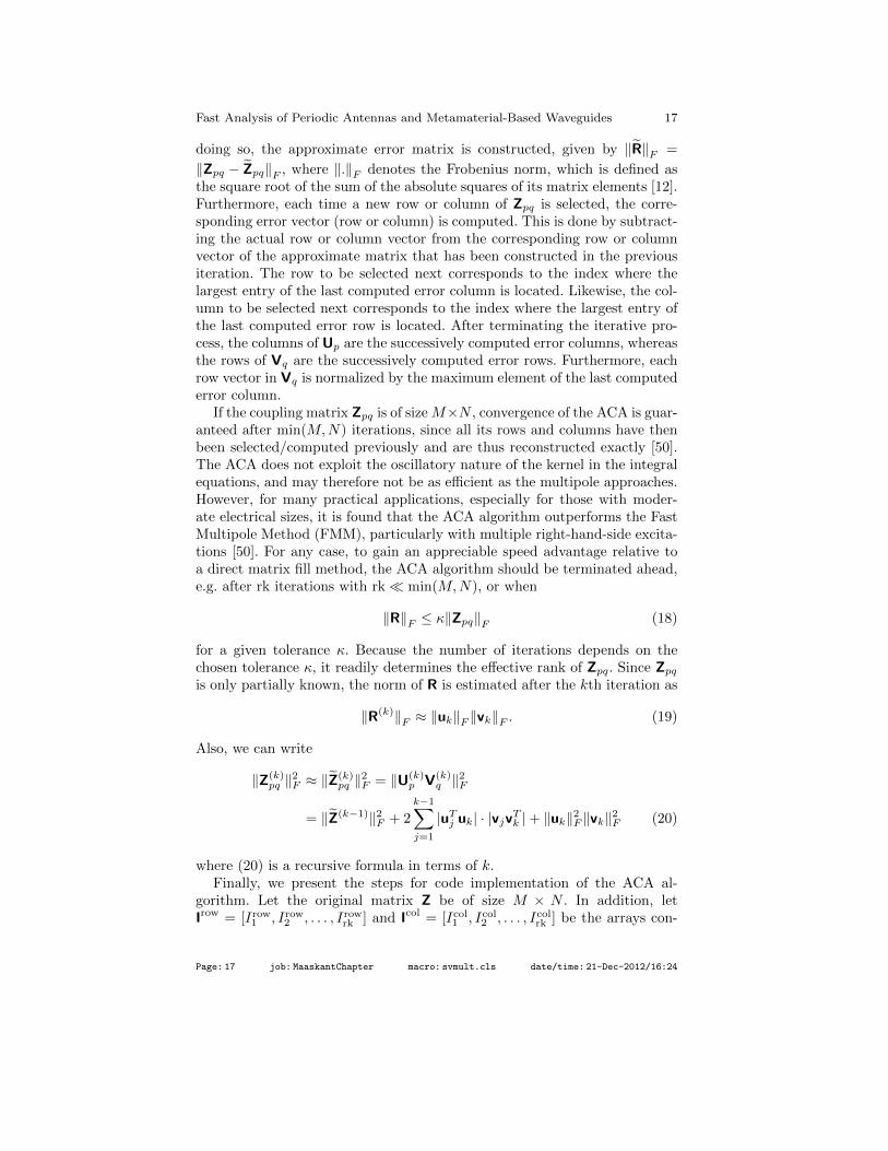
doing so, the approximate error matrix is constructed, given by ‖R‖F =
‖Zpq − Zpq‖F , where ‖.‖F denotes the Frobenius norm, which is defined asthe square root of the sum of the absolute squares of its matrix elements [12].Furthermore, each time a new row or column of Zpq is selected, the corre-sponding error vector (row or column) is computed. This is done by subtract-ing the actual row or column vector from the corresponding row or columnvector of the approximate matrix that has been constructed in the previousiteration. The row to be selected next corresponds to the index where thelargest entry of the last computed error column is located. Likewise, the col-umn to be selected next corresponds to the index where the largest entry ofthe last computed error row is located. After terminating the iterative pro-cess, the columns of Up are the successively computed error columns, whereasthe rows of Vq are the successively computed error rows. Furthermore, eachrow vector in Vq is normalized by the maximum element of the last computederror column.
If the coupling matrix Zpq is of size M×N , convergence of the ACA is guar-anteed after min(M,N) iterations, since all its rows and columns have thenbeen selected/computed previously and are thus reconstructed exactly [50].The ACA does not exploit the oscillatory nature of the kernel in the integralequations, and may therefore not be as efficient as the multipole approaches.However, for many practical applications, especially for those with moder-ate electrical sizes, it is found that the ACA algorithm outperforms the FastMultipole Method (FMM), particularly with multiple right-hand-side excita-tions [50]. For any case, to gain an appreciable speed advantage relative toa direct matrix fill method, the ACA algorithm should be terminated ahead,e.g. after rk iterations with rk min(M,N), or when
‖R‖F ≤ κ‖Zpq‖F (18)
for a given tolerance κ. Because the number of iterations depends on thechosen tolerance κ, it readily determines the effective rank of Zpq. Since Zpqis only partially known, the norm of R is estimated after the kth iteration as
‖R(k)‖F ≈ ‖uk‖F ‖vk‖F . (19)
Also, we can write
‖Z(k)pq ‖2F ≈ ‖Z(k)
pq ‖2F = ‖U(k)p V(k)
q ‖2F
= ‖Z(k−1)‖2F + 2
k−1∑j=1
|uTj uk| · |vjvTk |+ ‖uk‖2F ‖vk‖2F (20)
where (20) is a recursive formula in terms of k.Finally, we present the steps for code implementation of the ACA al-
gorithm. Let the original matrix Z be of size M × N . In addition, letIrow = [Irow1 , Irow2 , . . . , Irowrk ] and Icol = [Icol1 , Icol2 , . . . , Icolrk ] be the arrays con-
taining orderly selected row and column indices of Z, The vector uk representsthe kth column of the matrix U, and vk denotes the kth row of the matrixV. In Matlab’s notation, R(Irow1 , :) indicates the Irow1 th row of matrix R. Z(k)
is the matrix Z at the kth iteration. Then, in pseudo-Matlab code, the algo-rithm is summarized as follows [50]:
Initialization (k = 1):
1. Initialize the 1st row index Irow1 = 1 and set Z = 0.
2. Initialize the 1st row of the approx. error matrix: R(Irow1 , :) = Z(Irow1 , :).
4. Update the Icolk th column of R: R(:, Icolk ) = Z(:, Icolk )−k−1∑l=1
(vl)Icolkul.
5. uk = R(:, Icolk ).
6. ‖Z(k)‖2F = ‖Z(k−1)‖2F + 2k−1∑j=1
|uTj uk||vTj vk|+ ‖uk‖2F ‖vk‖2F .
7. Check convergence, if ‖uk‖F ‖vk‖F ≤ ε‖Z(k)‖F , end iteration.
8. Find the next row index Irowk+1 : |R(Irowk+1, Icolk )| = maxi (|R(i, Icolk )|), i 6=
Irow1 , . . . , Irowk .
4 Computation of Radiation and ImpedanceCharacteristics
4.1 Input Admittance Matrix
In most MoM formulations, the input admittance matrix can be convenientlycalculated, without additional manipulations, by using the induced surfacecurrents when the ports are excited by voltage sources, while all other termi-nals are short-circuited. The mutual admittance (or impedance) between two
Fast Analysis of Periodic Antennas and Metamaterial-Based Waveguides 19
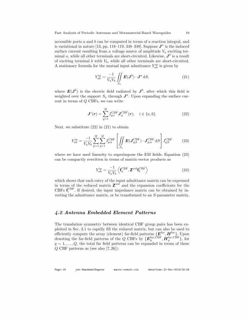
accessible ports a and b can be computed in terms of a reaction integral, andis variational in nature [13, pp. 118–119, 348–349]. Suppose Ja is the inducedsurface current resulting from a voltage source of amplitude Va exciting ter-minal a, while all other terminals are short-circuited. Likewise, Jb is a resultof exciting terminal b with Vb, while all other terminals are short-circuited.A stationary formula for the mutual input admittance Y in
ab is given by
Y inab =
−1
VaVb
∫Sa
∫E(Jb) · Ja dS, (21)
where E(Jb) is the electric field radiated by Jb, after which this field isweighted over the support Sa through Ja. Upon expanding the surface cur-rent in terms of Q CBFs, we can write
J i(r) =
Q∑q=1
ICBFq;i JCBF
q (r), i ∈ a, b. (22)
Next, we substitute (22) in (21) to obtain
Y inab =
−1
VaVb
Q∑p=1
Q∑q=1
ICBFp;a
∫Sa
∫E(JCBF
q;b ) · JCBFp;a dS
ICBFq;b (23)
where we have used linearity to superimpose the EM fields. Equation (23)can be compactly rewritten in terms of matrix-vector products as
Y inab =
−1
VaVb
⟨ICBFa ,ZredICBF
b
⟩(24)
which shows that each entry of the input admittance matrix can be expressedin terms of the reduced matrix Zred and the expansion coefficients for theCBFs ICBF
i . If desired, the input impedance matrix can be obtained by in-verting the admittance matrix, or be transformed to an S-parameter matrix.
4.2 Antenna Embedded Element Patterns
The translation symmetry between identical CBF group pairs has been ex-ploited in Sec. 3.1 to rapidly fill the reduced matrix, but can also be used toefficiently compute the array (element) far-field patterns Efar,H far. Upondenoting the far-field patterns of the Q CBFs by Efar,CBF
q ,H far,CBFq , for
q = 1, . . . , Q, the total far field patterns can be expanded in terms of theseQ CBF patterns as (see also [7, 26]):
where ICBFq is the qth expansion coefficient for the qth CBF current. The
coefficient vector ICBF is computed via the CBFM for a certain array excita-tion.
The approach outlined above is time-consuming if Q, the total numberof CBFs, is larger than the number of array elements times the number ofexcitation schemes considered. However, because many of the subdomainssupport the same set of CBFs, the respective CBF patterns are identical aswell, apart from a phase correction due to their translated position. Hence,translation symmetry can be exploited to compute the patterns pertainingto a few unique sets of CBFs only. For instance, we can write
Efar,CBFp ,H far,CBF
p = Efar,CBFq ,H far,CBF
q e−jk(rpq·r(θ,φ)) (26)
where the pth CBF pattern is derived from the qth one by accounting forthe translation vector rpq. The unit vector r(θ, φ) denotes the direction ofobservation, and k is the wavenumber of the homogenous medium. Note that,for our example (Fig. 4), we need to explicitly compute the CBF patterns forthe sets of CBFs supported only by the subdomains 1, 3 and 5. The remainingCBF patterns are simply obtained via translation.
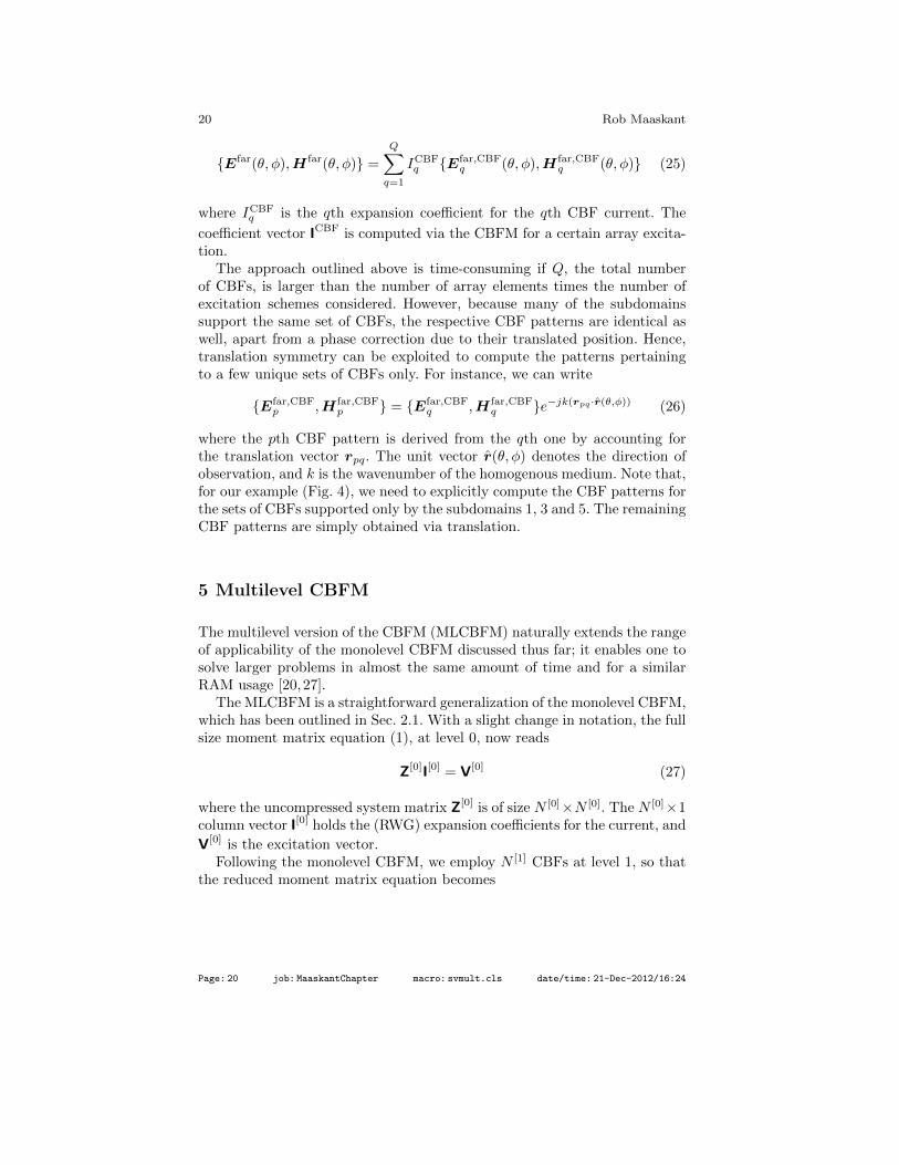
5 Multilevel CBFM
The multilevel version of the CBFM (MLCBFM) naturally extends the rangeof applicability of the monolevel CBFM discussed thus far; it enables one tosolve larger problems in almost the same amount of time and for a similarRAM usage [20,27].
The MLCBFM is a straightforward generalization of the monolevel CBFM,which has been outlined in Sec. 2.1. With a slight change in notation, the fullsize moment matrix equation (1), at level 0, now reads
Z[0]I[0] = V[0] (27)
where the uncompressed system matrix Z[0] is of size N [0]×N [0]. The N [0]×1column vector I[0] holds the (RWG) expansion coefficients for the current, and
V[0] is the excitation vector.Following the monolevel CBFM, we employ N [1] CBFs at level 1, so that
Fast Analysis of Periodic Antennas and Metamaterial-Based Waveguides 21
Z[1]I[1] = V[1], where the
sub-matrix: Z[1]mn =
⟨J[0]m ,Z
[0]mnJ[0]
n
⟩sub-vector: V[1]
m =⟨
J[0]m ,V
[0]m
⟩.
(28)
The matrix block Z[0]mn contains the interactions between a pair of RWG
groups, each of which supports a set of CBFs, e.g., J[0]m or J[0]
n , whose columnsare the RWG expansion coefficients describing a CBF on that subdomain. TheCBF-compressed matrix Z[1] is of size N [1] ×N [1]. Once the solution for I[1]
has been computed, the solution to the original problem, I[0], can be foundby using
I[0] =
N [1]∑m=1
I [1]m J[1],CBFm (29)
where
J[1],CBFm
are the entire-domain CBFs at level 1. These vectors con-
tain many zeros to make up the expansion coefficient vectors that are of sizeN [0] × 1. Next, we proceed this successive compression process for higherlevels, resulting in the following recursive scheme at level i:
Z[i]I[i] = V[i], where the
sub-matrix: Z[i]mn =
⟨J[i−1]m ,Z[i−1]
mn J[i−1]n
⟩sub-vector: V[i]
m =⟨
J[i−1]m ,V[i−1]
m
⟩.
(30)
where the solution at the lower level i−1 is expressed in terms of the solution
at level i and its set of CBFs, i.e., we can write I[i−1] =∑N [i]
m=1 I[i]mJ[i],CBF
m , fori = 1, 2, . . .
It is to be noted that a set of CBFs need to be generated at each level, andthis requires additional operations in comparison with a monolevel CBFM.In conclusion, the number of unknowns may be significantly reduced, but thespeed advantage becomes only apparent for electrically large problems [20].The numerical results section includes the challenging problem of a largearray of disjoint subarrays, where RWGs are employed at the lowest level,after which a set of CBFs is employed per antenna element at level 1, andwhere a set of CBFs is employed per subarray at level 2. We then solve theproblem at level 2, and obtain the currents at the lowest level by using therecursive scheme in (30).
6 Numerical Results
The following CBFM computations have been carried out on a 64 bit (x86-64)Linux – openSUSE (v.11.4) server equipped with 2 Intel Xeon E5640 CPUsoperating at 2.67 GHz (each CPU has 4 cores/8 threads), with access to 144
GB RAM memory and 2 TB harddisk space. The HFSS simulations wereperformed on a 64 bit Windows XP server equipped with 2 Intel Xeon 5130CPUs operating at 2 GHz (each CPU has 2 cores/2 threads), 8 GB RAM,and 300 GB harddisk space.
6.1 A 7 × 1 (Vivaldi) Tapered Slot Antenna Array
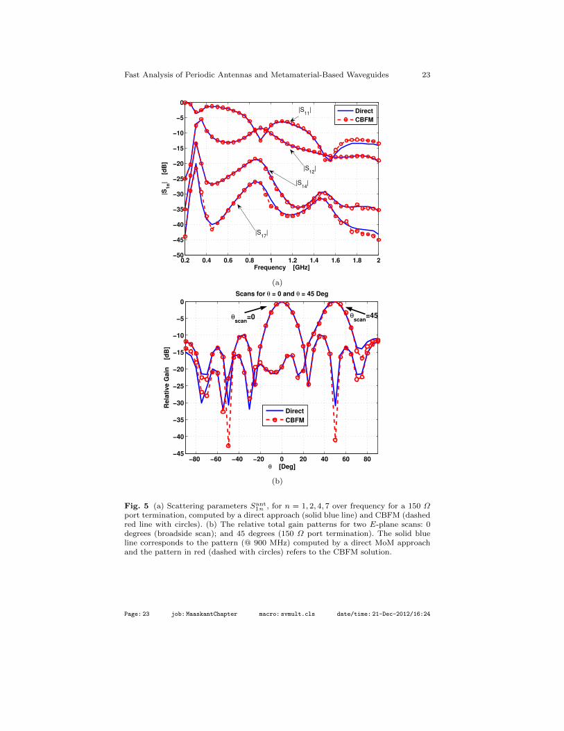
The numerical accuracy of the CBFM combined with the ACA will be as-sessed in this section for a 1-D singly-polarized array of electrically intercon-nected TSA elements3. The results are compared to a direct MoM solutionemploying RWG basis functions only. The CBFs are generated as describedin Sec. 2.2, where a threshold of 10−2 is used both for the SVD procedurein CBFM and the ACA algorithm. The radius for generating the secondaryCBFs has been chosen equal to the width of two elements, and has beenspecified to be independent of the frequency. Following the SVD procedure,only 3 CBFs are retained for the outer two corner elements and 5 CBFs forthe inner elements (@ 900 MHz). Figs. 5 and 6 show the computed resultsfor a 7× 1 array of TSAs.
In Fig. 5, one visually observes a very good agreement between the CBFMand direct solution for both the radiation and impedance characteristics.These results show that the electrical interconnection between TSA elementsis treated accurately, even though small differences are noticeable in the errorsurface current distribution JError
S [Fig. 6(b), top]. However, ‖JErrorS ‖2 is at
least 30 dB lower than the largest magnitude observed in ‖JMoMS ‖2, which is
found to be ∼ 12 dBA/m. The current is a smoothly varying function acrossthe common edge connecting both the element under excitation (#1) and itsdirect adjacent element (#2), whereas the current continuity degrades acrosscommon edges for elements farther out. This can be understood by realizingthat CBFs have been generated to accurately represent the current on theexcited element as well as on those elements that are directly adjacent (seegeneration of CBFs in Section 2.2). The all-excited array case demonstratestherefore a better continuity of the current across all the common edges.To reduce the error for the one-element excitation case, more CBFs need tobe generated to represent the rapidly varying current on the TSA elementsfarther out, at the cost of sacrificing the total execution time.
Fig. 6(b) (bottom) illustrates the average error of the RWG expansioncoefficients as a result of comparing the CBFM solution to a direct MoMsolution. This error is plotted as a function of frequency and refers to thecase that corner element 1 is excited by a voltage source while all others areshort-circuited; it is defined as
3 The accuracy of a more practical microstrip-fed 8 × 7 dual-polarized TSA arrayis discussed in [23], which involves a combination of electrodynamic and quasi-staticfield models [16].
Fast Analysis of Periodic Antennas and Metamaterial-Based Waveguides 23
0.2 0.4 0.6 0.8 1 1.2 1.4 1.6 1.8 2−50
−45
−40
−35
−30
−25
−20
−15
−10
−5
0
Frequency [GHz]
|S1
n|
[
dB
]
Direct
CBFM
|S11
|
|S12
|
|S14
|
|S17
|
(a)
−80 −60 −40 −20 0 20 40 60 80−45
−40
−35
−30
−25
−20
−15
−10
−5
0
Scans for θ = 0 and θ = 45 Deg
θ [Deg]
Re
lati
ve
Ga
in
[d
B]
θscan
=0 θscan
=45
Direct
CBFM
(b)
Fig. 5 (a) Scattering parameters Sant1n , for n = 1, 2, 4, 7 over frequency for a 150 Ω
port termination, computed by a direct approach (solid blue line) and CBFM (dashedred line with circles). (b) The relative total gain patterns for two E-plane scans: 0degrees (broadside scan); and 45 degrees (150 Ω port termination). The solid blueline corresponds to the pattern (@ 900 MHz) computed by a direct MoM approachand the pattern in red (dashed with circles) refers to the CBFM solution.
Fig. 6 (a) Magnitude of the normalized surface current distribution in [dBA/m] andport/element numbering for the direct solution and CBFM solution when element1 is excited by a voltage source and all other terminals are short-circuited (@ 900MHz). The difference between both current distributions is shown in (b), top, andthe average error between the RWG expansion coefficients over frequency is shown in(b), bottom.
Fast Analysis of Periodic Antennas and Metamaterial-Based Waveguides 25
Rel. Error =
√√√√ N∑n=1
∣∣IRWG,MoMn − IRWG,CBFM
n
∣∣2√√√√ N∑n=1
∣∣IRWG,MoMn
∣∣2 × 100%. (31)
On average, the relative error is less than 5% but may become larger asit tends to oscillate in accordance with the resonant behavior of the surfacecurrent. Obviously, near such a resonance, a small shift in frequency mayresult in a large relative error of the surface current. Resonances appearat almost constant intervals and weaken in strength as the array becomeselectrically large, resulting in a relative error that levels out below 5%. Forcompleteness, we also plot the reduced error curve when the SVD threshold islowered to 10−4. A close inspection of the corresponding current distributionreveals that the current improves globally, which also mitigates the problemof discontinuous behavior of the current across the common edges (althoughnot shown).
6.2 CBFM – ACA Hybridization Results
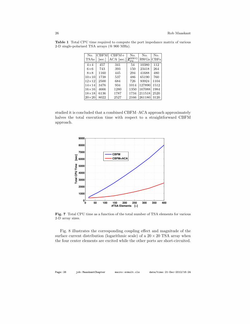
We consider the computational complexities of both the CBFM and CBFM +ACA approaches for analyzing large arrays of electrically interconnected TSAelements. The total CPU time required to compute the antenna impedancematrix of 2-D single-polarized arrays, ranging from 16 up to 400 TSA el-ements, is displayed in Table 1. The total CPU time includes the time togenerate primary and secondary CBFs, to perform the SVD, to constructand solve the reduced matrix equation, either with or without the ACA algo-rithm, and to compute the antenna impedance matrix. The total number ofmatrix blocks Zpq that need to be constructed remains relatively low. In fact,for a 400 element TSA array, 400 × 400 blocks need to be constructed butthis quantity is reduced to only 1199 (0.7%) by exploiting reciprocity andtranslation symmetry. Moreover, this number scales as O(N), where N isthe total number of TSA elements. Hence, for relatively small arrays, a largeportion of the time is devoted to the generation of CBFs, which implies thatthe speed advantage of the ACA algorithm becomes more apparent for verylarge arrays, or for arrays that exhibit little translation symmetry. Due to thefine geometrical features of a TSA element, as well as the utilized method togenerate CBFs (primaries+secondaries), the reduction factor of unknowns isquite significant (∼ 135).
For ease of comparison of the computational cost of CBFM to that of thecombined CBFM–ACA approach, the results of Table 1 have been graphicallyillustrated in Fig. 7. For the array configurations and sizes that we have
studied it is concluded that a combined CBFM–ACA approach approximatelyhalves the total execution time with respect to a straightforward CBFMapproach.
0 50 100 150 200 250 300 350 4000
1000
2000
3000
4000
5000
6000
7000
8000
9000
#TSA Elements [−]
To
tal
CP
U T
ime
[se
c]
CBFM
CBFM+ACA
Fig. 7 Total CPU time as a function of the total number of TSA elements for various2-D array sizes.
Fig. 8 illustrates the corresponding coupling effect and magnitude of thesurface current distribution (logarithmic scale) of a 20× 20 TSA array whenthe four center elements are excited while the other ports are short-circuited.
Fast Analysis of Periodic Antennas and Metamaterial-Based Waveguides 27
Fig. 8 Surface current distribution of a 20 × 20 TSA array (Magnitude in [dBA/m]@ 900 MHz). The four center elements are equally excited by voltage generators (1V) while the others are short-circuited.
6.3 Multilevel CBFM – Array of Subarray Antennas
It is conjectured that the solution for the current on the array of M disjointsubarrays can be accurately synthesized by those found on a single isolatedsubarray. If a single isolated subarray consists of N antenna elements, wefirst excite the N elements sequentially and compute the associated subar-ray currents using a monolevel CBFM approach to generate CBFs (level 1).Afterwards, these solutions so obtained/generated, are used as a set of pri-mary CBFs to synthesize the current distribution on each of the M disjointsubarrays (level 2). Hence, at the highest level we only have to solve forM × N unknown CBF expansion coefficients (per excitation), as opposedto the M × K CBFs that would be required for a monolevel CBFM (withK N), where K is the total number of CBFs needed to synthesize thecurrent on a single subarray (level 1).
The numerical accuracy and efficiency of a two-level CBFM approach, rel-ative to a monolevel one, will be evaluated in this section for an array of25 disjoint subarrays of 64 TSA elements each. These gaps may need to beintroduced for servicing purposes, so that the individual subarrays can beinstalled and/or removed as modular units. Furthermore, the transport andmanufacturability of relatively small units may offer an advantage. Addition-ally, an accurate analysis of these nested antenna arrays is important as well,since the gaps/slots between disjoint subarray tiles tend to resonate and leadto anomalous antenna impedance effects as discussed in [36,37].
Numerical computations have been performed for an SVD threshold levelof 10−2 (used to reduce and retain a minimal set of basis function at each level
of the MLCBFM). The ACA threshold, which is used to rapidly constructthe low-rank (off-diagonal) moment matrix blocks, has been set to 10−3.Numerical experiments have shown that a reduced ACA threshold level has apositive effect on the symmetry of the input impedance matrix. Furthermore,it suppresses the spurious ripples that the element radiation patterns mayexhibit, albeit at a cost of longer matrix fill-time. At level 1, the radius forgenerating the secondary CBFs has been taken equal to the width of twoantenna elements, whereas it has been enlarged at level-2 to incorporate allthe surrounding subarrays. We have also studied the case in which we bypassthe generation of secondary CBFs at level-2.
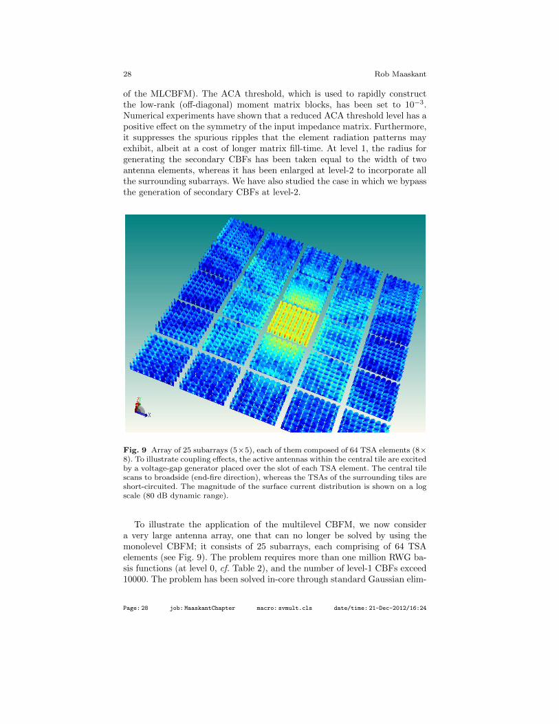
Fig. 9 Array of 25 subarrays (5×5), each of them composed of 64 TSA elements (8×8). To illustrate coupling effects, the active antennas within the central tile are excitedby a voltage-gap generator placed over the slot of each TSA element. The central tilescans to broadside (end-fire direction), whereas the TSAs of the surrounding tiles areshort-circuited. The magnitude of the surface current distribution is shown on a logscale (80 dB dynamic range).
To illustrate the application of the multilevel CBFM, we now considera very large antenna array, one that can no longer be solved by using themonolevel CBFM; it consists of 25 subarrays, each comprising of 64 TSAelements (see Fig. 9). The problem requires more than one million RWG ba-sis functions (at level 0, cf. Table 2), and the number of level-1 CBFs exceed10000. The problem has been solved in-core through standard Gaussian elim-
Fast Analysis of Periodic Antennas and Metamaterial-Based Waveguides 29
ination techniques at level-2, where the number of CBFs is as low as 3100.The total execution time is just over 11 hours, most of which is devoted tofilling the blocks of the moment matrix. Approximate times for assemblingthe reduced matrix was ∼176 min; computing the reduced set of excitationvectors ∼103 min; solving the reduced matrix at level-2 (3100 × 3100) andcomputing the antenna impedance matrix ∼22 min, and the remaining timehas been spent on the generation of the primary and secondary CBFs. It isworthwhile to point out that the mesh generation took only 18 min and 9 sec,because advantage was taken of the fact that a large degree of translationsymmetry exists at all levels for regularly-spaced antenna arrays.
Table 2 Required computational resources and execution time for a level-2 CBFMapproach.
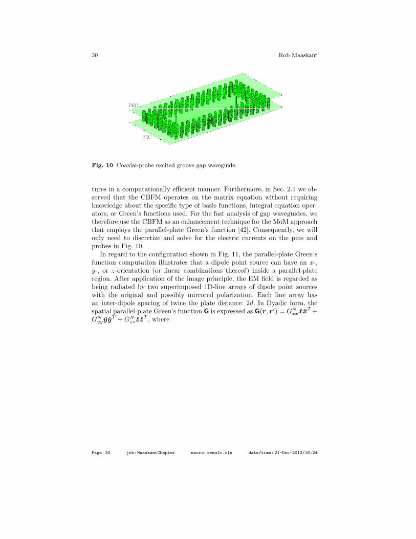
Recently, a novel class of low-loss low-cost waveguide and transmission-linetechnologies have been introduced to anticipate to future demands in high-frequency electronics. These structures utilize periodic structures for guidingthe fields along desired paths, while incorporating filtering mechanisms andtransitions to other waveguides and/or transmission lines at the same time.Furthermore, they allow for a high degree of integration with active elec-tronic components. One of the most profound examples are the recently in-vented Substrate Integrated Waveguide (SIW, [5]) and Gap Waveguide struc-tures [17]. We will focus on the latter one, whose basic structure consists ofa pair of perfect electric conducting (PEC) top and bottom ground planes inconjunction with a periodic texture of metallic objects synthesizing the meta-material. Fig. 10 depicts the so-called groove gap waveguide [28], where twocoaxial probes are used to excite the waveguide fields. The groove is borderedby only a few rows of pins which prevent the fields from leaking out (side-ways), provided that we operate in the stop band. The pins are electricallyinterconnected to the bottom PEC plate, while no electrical contact betweenthe pins and the upper PEC plate is required. The above capacitive gap in theso-called “gap waveguide” not only emulates a perfect magnetic conductor(PMC) boundary condition, but represents a mechanical advantage as well.
As explained above, the CBFM is an enhancement technique for themethod of moments and is very well suited to deal with large periodic struc-
Fig. 10 Coaxial-probe excited groove gap waveguide.
tures in a computationally efficient manner. Furthermore, in Sec. 2.1 we ob-served that the CBFM operates on the matrix equation without requiringknowledge about the specific type of basis functions, integral equation oper-ators, or Green’s functions used. For the fast analysis of gap waveguides, wetherefore use the CBFM as an enhancement technique for the MoM approachthat employs the parallel-plate Green’s function [42]. Consequently, we willonly need to discretize and solve for the electric currents on the pins andprobes in Fig. 10.
In regard to the configuration shown in Fig. 11, the parallel-plate Green’sfunction computation illustrates that a dipole point source can have an x-,y-, or z-orientation (or linear combinations thereof) inside a parallel-plateregion. After application of the image principle, the EM field is regarded asbeing radiated by two superimposed 1D-line arrays of dipole point sourceswith the original and possibly mirrored polarization. Each line array hasan inter-dipole spacing of twice the plate distance: 2d. In Dyadic form, thespatial parallel-plate Green’s function G is expressed as G(r, r′) = GNxxxx
Fast Analysis of Periodic Antennas and Metamaterial-Based Waveguides 31
x
r
PEC
PEC
J = Iℓδ(r − r′)z
r′z d
r
PEC
PECr′
J = Iℓδ(r − r′)x
(a) (b)
r
2d
zx
n = 0
n = 1
r
2d
n = 0
n = 1
(c) (d)
Fig. 11 (a) z-polarized and (b) x-polarized electric Hertzian dipole currents in be-tween two infinitely large parallel PEC plates separated by a distance d; (c) and(d), the repeated application of the image principle for both dipole polarizations,respectively.
for N →∞, and where ρ2 = (x−x′)2 + (y− y′)2. The spatial summations inEq. (32) are known to be slowly convergent, however, each summation can becomputed rapidly using the Shanks transformation [38]. This method is easyto implement and very fast if only a few digits of accuracy is required, whichis sufficient in most practical cases [42]. For example, when considering thenew series G1
xx, G2xx, . . ., the Shanks-extrapolated value for G∞xx is
G∞xx ≈GN+1xx GN−1xx −
(GNxx
)2GN+1xx − 2GNxx +GN−1xx
(33)
where N is taken sufficiently large. Numerical experiments show that the besttrade-off between the solution accuracy and the total series evaluation timeis to use the doubly repeated Shanks transformation, which only requiresN ≈ 5 terms [42].
The electric surface currents on the pins and coaxial probes, of the guidingstructure shown in Fig. 10, are expanded in terms of 37088 RWG basis func-tions. The CBFs are generated only for a single pin and for the coaxial probe.As an example, consider Fig. 12(a), where the CBFs are generated for a pinin isolation by employing 382 RWGs. We let a PWS be incident on the pinwith angular increments of ∆θi = ∆φi = 900 (and two polarizations), whichgenerates 16 currents. The generated pin currents are stored as RWG expan-sion coefficients vectors and make up the columns of the matrix Jq = UDQH ,where the right-hand side is the SVD of Jq [see also Eq. (8)]. The magnitudeof the normalized singular values in D are plotted in Fig. 12(a). With anappropriate thresholding procedure on the singular values, only the first 12column vectors of the left-singular matrix U are retained, and subsequentlyused as CBFs. The reduction in the number of unknowns per pin is therefore382/12=31.8 (@ 12 GHz). We exploit the translation symmetry to generatea set of CBFs for all the pins, since the set of CBFs is identical for eachpin, and since this allows also for a rapid construction of the reduced matrix(see Sec. 3.1). A similar CBF generation procedure is followed for the coaxialprobes.
After all the pins and probes support a set of CBFs, the reduced momentmatrix equation ZredICBF = Vred is constructed, where Vred is a result ofexciting the structure by impressed magnetic frill currents that are supportedby the coaxial apertures.
The remaining geometrical dimensions of the groove gap waveguide areas described in Fig. 12(b). Additionally, the radius and length of the coaxialprobes are 0.25 and 5 mm, respectively, and the parallel-plate separationdistance d = 7.25 mm.
To examine the numerical accuracy, the 100-Ohm S-parameters for thegap waveguide structure in Fig. 12(b) have been computed through bothCBFM and the HFSS software. In HFSS, the adaptive meshing terminatesif the relative field error is less than 1%. The computed S-parameters forCBFM and HFSS are shown in Fig. 13 and are seen to be in good agreement.
Fast Analysis of Periodic Antennas and Metamaterial-Based Waveguides 33
2 4 6 8 10 12 14 16 18 2010
−15
10−10
10−5
100
n [−]
σn/σ
ma
x
[−
]
Singular Values
Threshold
PWS
∆θi = 900
∆φi = 900
(a)
Wpin Hpin L1 L2 L3 L4
1 6.25 15.8 43.7 5.4 2
Wpin
L3
L4
dprobe
L2
L1
(b)
Fig. 12 (a) Generation of CBFs on a pin using a plane wave spectrum (PWS). Thesingular value spectrum is shown where a threshold is used to limit the maximumnumber of employed CBFs. (b) Geometrical dimensions of the Groove gap waveguidein [mm].
The solve times for this relatively small problem is 1 min. 41 sec. and 1min. 24 sec. for CBFM and HFSS, respectively. The simulation times arecomparable due to the relatively large overhead needed by the CBFM todetermine the CBFs. The CBFM employed 1112 CBFs (37088 RWGs), whileHFSS employed 42158 tetrahedra. Owing to the nature of the array structure,the meshing time is only 5 sec. for the CBFM, while it takes 3 min. 57 sec.for HFSS.
−0.03−0.02
−0.010
0.010.02
−0.01
0
0.01
0
0.005
0.01
x [m]
Magnitude of Averaged Current Distribution[dBA/m or dBV/m] at f=12GHz
y [m]
z [m
]
−27.0303
−7.0303
12.9697
32.9697
52.9697
72.9697
10 12 14 16 18 20−60
−50
−40
−30
−20
−10
0
Zo=100 Ω
Frequency [GHz]
|S|
[
dB
]
|S11| CBFM
|S21| CBFM
|S11| HFSS
|S21| HFSS
(a) (b)
Fig. 13 (left) the magnitude of the computed electric current and S-parameters of agroove gap-waveguide when excited by a pair of coaxial probes; (right) the numericalresults are computed by the CBFM employing the parallel-plate Green’s function.The numerically computed results are validated through the HFSS software.
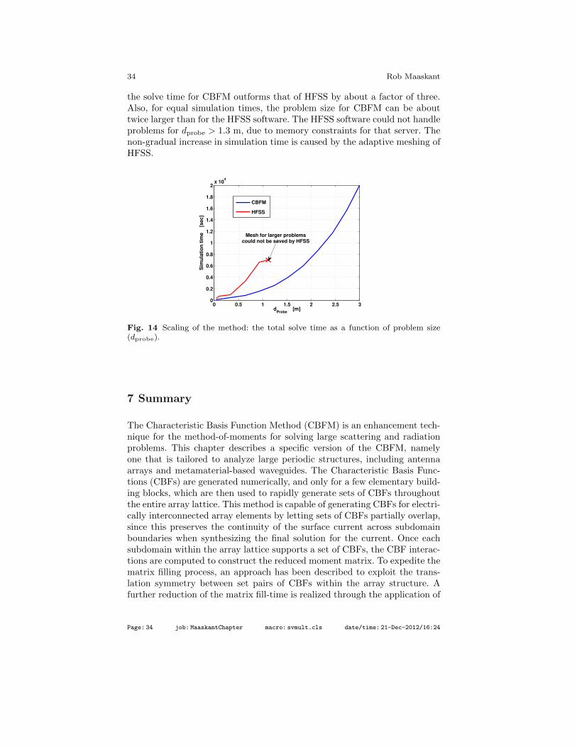
Next, by changing L2 one can examine the total solve time as a functionof the problem size. The results are shown in Fig. 14, where the scaling of
the solve time for CBFM outforms that of HFSS by about a factor of three.Also, for equal simulation times, the problem size for CBFM can be abouttwice larger than for the HFSS software. The HFSS software could not handleproblems for dprobe > 1.3 m, due to memory constraints for that server. Thenon-gradual increase in simulation time is caused by the adaptive meshing ofHFSS.
0 0.5 1 1.5 2 2.5 30
0.2
0.4
0.6
0.8
1
1.2
1.4
1.6
1.8
2x 10
4
dProbe
[m]
Sim
ula
tio
n t
ime [s
ec]
CBFM
HFSS
Mesh for larger problemscould not be saved by HFSS
Fig. 14 Scaling of the method: the total solve time as a function of problem size(dprobe).
7 Summary
The Characteristic Basis Function Method (CBFM) is an enhancement tech-nique for the method-of-moments for solving large scattering and radiationproblems. This chapter describes a specific version of the CBFM, namelyone that is tailored to analyze large periodic structures, including antennaarrays and metamaterial-based waveguides. The Characteristic Basis Func-tions (CBFs) are generated numerically, and only for a few elementary build-ing blocks, which are then used to rapidly generate sets of CBFs throughoutthe entire array lattice. This method is capable of generating CBFs for electri-cally interconnected array elements by letting sets of CBFs partially overlap,since this preserves the continuity of the surface current across subdomainboundaries when synthesizing the final solution for the current. Once eachsubdomain within the array lattice supports a set of CBFs, the CBF interac-tions are computed to construct the reduced moment matrix. To expedite thematrix filling process, an approach has been described to exploit the trans-lation symmetry between set pairs of CBFs within the array structure. Afurther reduction of the matrix fill-time is realized through the application of
Fast Analysis of Periodic Antennas and Metamaterial-Based Waveguides 35
the Adaptive Cross Approximation (ACA) algorithm. Finally, to be able toanalyze extremely large nested array structures, a multilevel version of themonolevel CBFM is described for achieving an even higher compression ofthe reduced moment matrix.
The numerical results demonstrate that the solutions for the antenna arraycurrent, the antenna input impedance matrix, and the radiation characteris-tics are in very good agreement with those obtained by using a direct MoMapproach, while the reduction factor in the number of basis functions for amonolevel CBFM approach – relative to a direct MoM approach – are sig-nificant, i.e., typically two-to-three orders in magnitude. The CBFM can beexplained as an algebraic method for solving large matrix equations and,hence, does not depend on the nature of the Green’s function. This has beendemonstrated for a metamaterial-based gap waveguide analyzed through aMoM approach employing the parallel-plate Green’s function. Very large gapwaveguides are analyzed, those that are far beyond the reach of commerciallyavailable software codes, such as HFSS, without comprising the solution ac-curacy much, as demonstrated for smaller more tractable problems.
References
1. Bebendorf, M.: Approximation of boundary element matrices. Numer. Math.86(4), 565–589 (2000)
2. Bekers, D.J., van Eijndhoven, S.J.L., van de Ven, A.A.F., Borsboom, P.P., Ti-jhuis, A.G.: Eigencurrent analysis of resonant behavior in finite antenna arrays.IEEE Trans. Microw. Theory Tech. 54(6), 2821–2829 (2006)
3. Bleszynski, E., Bleszynski, M., Jaroszewicz, T.: AIM: Adaptive integral methodfor solving large-scale electromagnetic scattering and radiation problems. RadioSci. 31(5), 1225–1251 (1996)
4. Boryssenko, A.O.: private communication (2004)5. Bozzi, M., Georgiadis, A., Wu, K.: Review of substrate-integrated waveguide
circuits and antennas. Microwaves, Antennas & Propagation, IET 5(8), 909–920(2011)
6. Civi, O.A., Pathak, P.H., Chou, H.T., Nepa, P.: A hybrid uniform geometricaltheory of diffraction – moment method for efficient analysis of electromagneticradiation/scattering from large finite planar arrays. Radio Sci. 35(2), 607–620(2000)
7. Craeye, C.: A fast impedance and pattern computation scheme for finite antennaarrays. IEEE Trans. Antennas Propag. 54(10), 3030–3034 (2006)
8. Craeye, C., Tijhuis, A.G., Schaubert, D.H.: An efficient MoM formulation forfinite-by-ininite arrays of two-dimensional antennas arranged in a three dimen-sional structure. IEEE Trans. Antennas Propag. 51(9), 2054–2056 (2003)
9. Delaunay, B.: Sur la sphere vide. Izvestia Akademii Nauk SSSR, OtdelenieMatematicheskikh i Estestvennykh Nauk 7, 793–800 (1934)
10. Delgado, C., Catedra, M.F., Mittra, R.: Efficient multilevel approach for the gen-eration of characteristic basis functions for large scatters. IEEE Trans. AntennasPropag. 56(7), 2134–2137 (2008)
11. Garcia, E., Delgado, C., de Adana, F.S., Catedra, F., Mittra, R.: Incorporat-ing the multilevel fast multipole method into the characteristic basis function
method to solve large scattering and radiation problems. In: Proc. IEEE AP-SInternational Symposium, pp. 1285–1288. Honulullu, Hawaii (2007)
12. Golub, G.H., van Loan, C.F.: Matrix Computations. 3rd ed. Baltimore, MD:Johns Hopkins, London (1996)
13. Harrington, R.F.: Time-Harmonic Electromagnetic Fields. McGraw-Hill BookCompany, New York and London (1961)
14. Harrington, R.F.: Field Computation by Moment Methods. The Macmillan Com-pany, New York (1968)
15. Heinstadt, J.: New approximation technique for current distribution in microstriparray antennas. Micr. Opt. Technol. 29, 1809–1810 (1993)
16. Ivashina, M.V., Redkina, E.A., Maaskant, R.: An accurate model of a wide-band microstrip feed for slot antenna arrays. In: Proc. IEEE AP-S InternationalSymposium, pp. 1953–1956. Hawaii, USA (2007)
17. Kildal, P.S., Alfonso, E., Valero-Nogueira, A., Rajo-Iglesias, E.: Localmetamaterial-based waveguides in gaps between parallel metal plates. IEEEAntennas Wireless Propag. Lett. 8(1), 84–87 (2009)
19. Lancellotti, V., de Hon, B.P., Tijhuis, A.G.: An eigencurrent approach to theanalysis of electrically large 3-d structures using linear embedding via green”soperators. IEEE Trans. Antennas Propag. 57(11), 3575–3585 (2009)
20. Laviada, J., Las-Heras, F., Pino, M.R., Mittra, R.: Solution of electrically largeproblems with multilevel characteristic basis functions. IEEE Trans. AntennasPropag. 57(10), 3189–3198 (2009)
21. Lu, W.B., Cui, T.J., Qian, Z.G., Yin, X.X., Hong, W.: Accurate analysis oflarge-scale periodic structures using an efficient sub-entire-domain basis functionmethod. IEEE Trans. Antennas Propag. 52(11), 3078–3085 (2004)
22. Maaskant, R.: Analysis of large antenna systems. Ph.D. thesis, Eindhoven Univer-sity of Technology, Eindhoven (2010). URL http://alexandria.tue.nl/extra2/
201010409.pdf
23. Maaskant, R., Ivashina, M.V., Iupikov, O., Redkina, E.A., Kasturi, S., Schaubert,D.H.: Analysis of large microstrip-fed tapered slot antenna arrays by combiningelectrodynamic and quasi-static field models. IEEE Trans. Antennas Propag.56(6), 1798–1807 (2011)
24. Maaskant, R., Mittra, R., Tijhuis, A.G.: Application of trapezoidal-shaped char-acteristic basis functions to arrays of electrically interconnected antenna elements.In: Proc. Int. Conf. on Electromagn. in Adv. Applicat. (ICEAA), pp. 567–571.Torino (2007)
25. Maaskant, R., Mittra, R., Tijhuis, A.G.: Fast analysis of large antenna arraysusing the characteristic basis function method and the adaptive cross approxi-mation algorithm. IEEE Trans. Antennas Propag. 56(11), 3440–3451 (2008)
26. Maaskant, R., Mittra, R., Tijhuis, A.G.: Fast solution of multi-scale antennaproblems for the square kilomtre array (SKA) radio telescope using the charac-teristic basis function method (CBFM). Applied Computational ElectromagneticsSociety (ACES) Journal 24(2), 174–188 (2009)
27. Maaskant, R., Mittra, R., Tijhuis, A.G.: Multilevel characteristic basis functionmethod (MLCBFM) for the analysis of large antenna arrays. Special Section onComputational Electromagnetics for Large Antenna Arrays, The Radio ScienceBullentin 336(336), 23–34 (2011)
28. Maaskant, R., Takook, P., Kildal, P.S.: Fast analysis of gap waveguides using thecharacteristic basis function method and the parallel-plate green’s function. In:Proc. Int. Conf. on Electromagn. in Adv. Applicat. (ICEAA), pp. 788–791. CapeTown (2012)
30. Matekovits, L., Vecchi, G., Bercigli, M., Bandinelli, M.: Synthetic-functions anal-ysis of large aperture-coupled antennas. IEEE Trans. Antennas Propag. 57(7),1936–1943 (2009)
31. Matekovits, L., Vecchi, G., Dassano, G., Orefice, M.: Synthetic function analysisof large printed structures: the solution space sampling approach. In: Proc. IEEEAP-S International Symposium, pp. 568–571. Boston, Massachusetts (2001)
32. Mittra, R., Ma, J.F., Lucente, E., Monorchio, A.: CBMOM–an iteration free MoMapproach for solving large multiscale em radiation and scattering problems. In:Proc. IEEE AP-S International Symposium, pp. 2–5. Washington DC (2005)
33. Neto, A., Maci, S., Vecchi, G., Sabbadini, M.: A truncated Floquet wave diffrac-tion method for the full wave analysis of large phased arrays – part ii: General-ization to 3-D cases. IEEE Trans. Antennas Propag. 48(3), 601–611 (2000)
34. Prakash, V., Mittra, R.: Characteristic basis function method: A new techniquefor efficient solution of method of moments matrix equations. Micr. Opt. Technol.36, 95–100 (2003)
35. Rao, S., Wilton, D., Glisson, A.: Electromagnetic scattering by surfaces of arbi-trary shape. IEEE Trans. Antennas Propag. 30(3), 409–418 (1982)
36. Schaubert, D.H., Boryssenko, A.O.: Subarrays of Vivaldi antennas for very largeapertures. In: Proc. 34th European Microwave Conference, pp. 1533–1536. Am-sterdam (2004)
37. Schaubert, D.H., Kasturi, S., Elsallal, M.W., van Cappellen, W.A.: Wide band-width Vivaldi antenna arrays – some recent developments. In: Proc. EuropeanConference on Antennas and Propag. (EuCAP), pp. 1–4. Nice, France (2006)
38. Shanks, D.: Non-linear transformation of divergent and slowly convergent se-quences. J. Math. Phys. 34, 1–42 (1955)
39. Skrivervik, A.K., Mosig, J.R.: Analysis of finite phased arrays of microstrippatches. IEEE Trans. Antennas Propag. 41(9), 1105–1114 (1993)
40. Stevanovic, I., Mosig, J.R.: Subdomain multilevel approach with fast MBF inter-actions. In: Proc. IEEE AP-S International Symposium, pp. 367–370. Monterey,California (2004)
41. Suter, E., Mosig, J.R.: A subdomain multilevel approach for the efficient MoManalysis of large planar antennas. Micr. Opt. Technol. 26(4), 270–277 (2000)
42. Takook, P., Maaskant, R., Kildal, P.S.: Comparison of parallel-plate greens func-tion acceleration techniques. In: Proc. European Conference on Antennas andPropag. (EuCAP), pp. 1–5. Prague, Czech Republic (2012)
43. Tiberi, G., Monorchio, A., Manara, G., Mittra, R.: Hybridizing asymptotic andnumerically rigorous techniques for solving electromagnetic scattering problemsusing the characterisitic basis functions (CBFs). In: Proc. IEEE AP-S Interna-tional Symposium, pp. 22–27. Columbus, Ohio (2003)
44. Tomasic, B., Hessel, A.: Analysis of finite arrays – a new approach. IEEE Trans.Antennas Propag. 47(3), 555–564 (1999)
45. Trefethen, L.N., Bau, D. (eds.): Numerical Linear Algebra. Society for Industrialand Applied Mathematics (SIAM), Philadelphia (1997)
46. Vandenbosch, G.A.E., Demuynck, F.J.: The expansion wave concept – part ii: Anew way to model mutual coupling in microstrip arrays. IEEE Trans. AntennasPropag. 46(3), 407–413 (1998)
47. Vandenbosch, G.A.E., Van de Cappelle, A.R.: Use of combined expansion schemeto analyze microstrip antennas with the method of moments. Radio Sci. 27(6),911–916 (1992)
48. Vita, P.D., Freni, A., Matekovits, L., Pirinoli, P., Vecchi, G.: A combinedAIM-SFX approach for large complex arrays. In: Proc. IEEE AP-S InternationalSymposium, pp. 3452–3455. Honulollu, Hawaii (2007)
49. Yeo, J., Prakash, V., Mittra, R.: Efficient analysis of a class of microstrip antennasusing the characteristic basis function method (CBFM). Micr. Opt. Technol. 39,456–464 (2003)
50. Zhao, K., Vouvakis, M.N., Lee, J.F.: The adaptive cross approximation algorithmfor accelerated method of moments computations of EMC problems. IEEE Trans.Electromagn. Compat. 47(4), 763–773 (2005)