92
Chanan Singh Regents Professor Department of Electrical and Computer Engineering Texas A&M University College Station, TX 77843, USA DLP : Bangkok, Dec 14, 2017

Chanan SinghRegents Professor
Department of Electrical and Computer EngineeringTexas A&M University
College Station, TX 77843, USA
DLP : Bangkok, Dec 14, 2017

Modern power systems are integration of Physical part, or primary part consisting
of current carrying components for power delivery and Cyber part or secondary part consisting of
monitoring, computing, communication and protection systems.
Human interface - power systems are not fully automated.
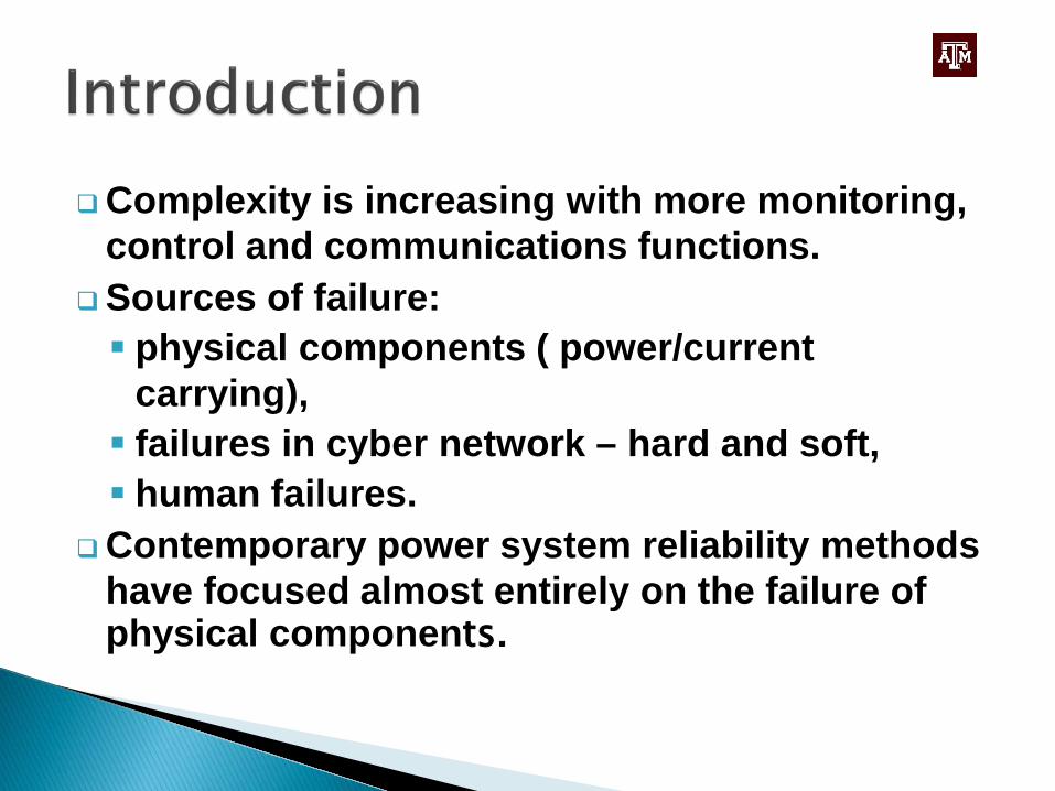
Complexity is increasing with more monitoring, control and communications functions.
Sources of failure: physical components ( power/current
carrying), failures in cyber network – hard and soft, human failures.
Contemporary power system reliability methods have focused almost entirely on the failure of physical components.


Power systems of the future are emerging to be different.
Two major factors contributing to this change: Large penetration of renewable energy sources Increasing complexity of cyber part.
Installation of hardware for interactive relationship between the supplier and consumer will add to complexity and interdependency between the cyber and physical parts.
Complexity and interdependency will introduce more sources of problems and make reliability analysis more challenging but also more essential.
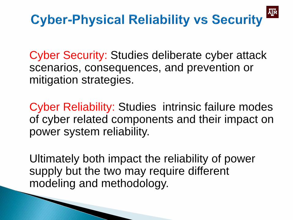
Cyber Security: Studies deliberate cyber attack scenarios, consequences, and prevention or mitigation strategies.
Cyber Reliability: Studies intrinsic failure modes of cyber related components and their impact on power system reliability.
Ultimately both impact the reliability of power supply but the two may require different modeling and methodology.

Think before you act. Analyze before you construct or implement. Analysis at the planning and design stage
leads to cost effective decisions that assure appropriate levels of reliability.
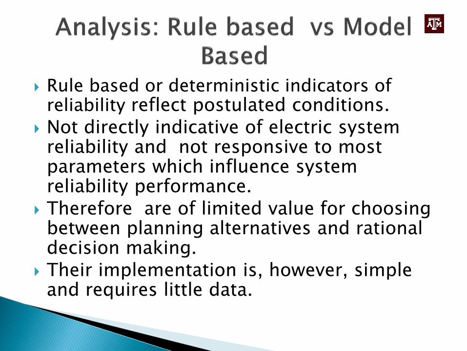
Rule based or deterministic indicators of reliability reflect postulated conditions.
Not directly indicative of electric system reliability and not responsive to most parameters which influence system reliability performance.
Therefore are of limited value for choosing between planning alternatives and rational decision making.
Their implementation is, however, simple and requires little data.
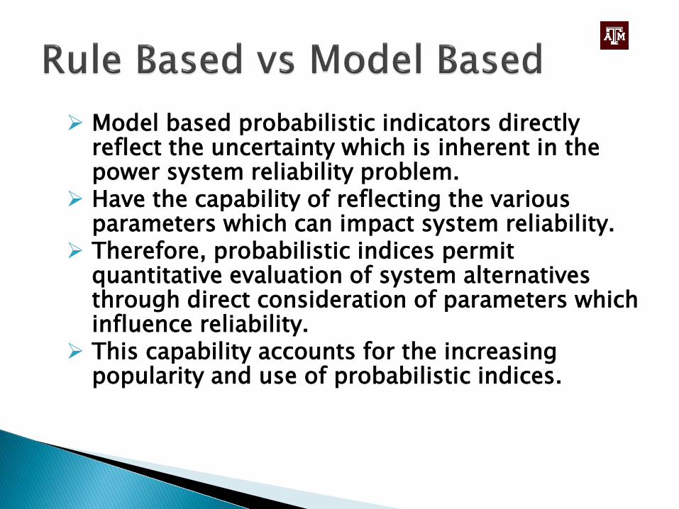
Model based probabilistic indicators directly reflect the uncertainty which is inherent in the power system reliability problem.
Have the capability of reflecting the various parameters which can impact system reliability.
Therefore, probabilistic indices permit quantitative evaluation of system alternatives through direct consideration of parameters which influence reliability.
This capability accounts for the increasing popularity and use of probabilistic indices.

System coverage: What part of the system is modeled.
Solution approaches: ◦ What models are used and◦ the mathematical methods employed for their
solution.

Generating capacity reliability evaluation(HL1): basic objective is to determine adequacy of generation to meet demand with a given probability. Single area: Transmission assumed capable of
transporting power from generation to load. Conceptually all generation and load in an area assumed connected to one bus.
Multi-area: Inter-area tie line constraints are considered. Intra-area constraints considered only indirectly.

Generation
Load
Area 1 Area 2
Area 4Area 3
Single Area Model
Multi Area Model

Composite system reliability evaluation(HL2): joint treatment of generation and bulk transmission. Constraints imposed by the capacity and impedance of
transmission lines are considered. Voltage constraints may also be considered
Distribution system reliability(HL3): given the reliability at distribution substation, determine the reliability at customer level.
Special topics: reliability of protection systems and their impact on system reliability.

Composite System Model Distribution System

Analytical methods: mostly used in single, multi-area and distribution system models.
Monte Carlo simulation; mostly used in multi-area and composite system models.
Intelligent search techniques: still in development stage for either increasing the efficiency of analytical or simulation or providing an alternative to Monte Carlo simulation.

Hybrid: mixing of different approaches for increased flexibility and strength.
Two of assumptions running through the developed models and methods :◦ independence of components.◦ cyber part is perfectly reliable and always
functions as it should.

State Selection
Evaluation
Reliability IndicesCalculation
Unit & System Models
Operating Strategies
LoadCurtailment
Success State Failure State
G1 G2 G3
G4
G5L1 L2
L3
L4

System model complexity depend upon the intended application.
For single area studies the model is fairly simple unless operating considerations are included.
For multi-area studies the system model is more complex.
Presently composite level represents the highest level of complexity. Even at this level, complicating issues like the impact
of protective relay malfunctions is generally excluded.
Load is assumed forecast and its responsiveness to market conditions and type of generation available is not modeled in detail.

Not possible to consider all system states because of dimensionality issue.
Analytical methods try to meet challenge of dimensionality by state merging, truncation and implicit enumeration.
Monte Carlo simulation meets this challenge by sampling.
Recently emerging intelligent search techniques, focus is on identifying dominant failure states.

Success States
Dominant FailedStates
Non-dominantFailed States

In any method, the selected state needs to be evaluated to determine if the objectives of the system are satisfied.
This may be simple addition or subtraction. This may need a transportation type model. Or more time consuming DC or AC power
flow model.

Non-sequential or sampling. Sequential simulation.

Sample component states proportional to their probabilities.
Construct system states from component states.
Evaluate system states. Estimate indices.

Step 1: Set the initial state of all components as UP and set the simulation time t = 0.
Step 2: For each component, draw a random decimal number between 0 and 1 and using random number and transition rate determine the time to next transition of each component.

Step 3: Find the minimum time to transition, change the state of the corresponding component q, and update the total time.
Step 4: Change the qth component’s state accordingly.
Step 5: Perform a network power flow analysis to assess system operation states. Update system-wide reliability indices.
Repeat steps 2–5 until convergence is achieved
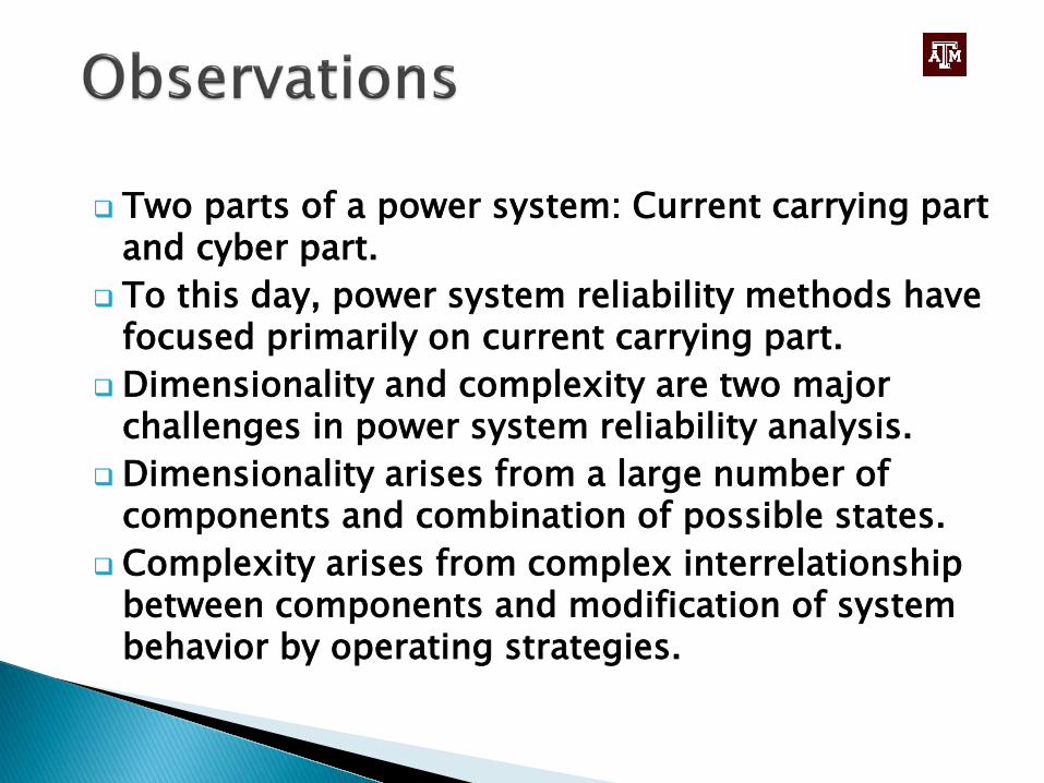
Two parts of a power system: Current carrying part and cyber part.
To this day, power system reliability methods have focused primarily on current carrying part.
Dimensionality and complexity are two major challenges in power system reliability analysis.
Dimensionality arises from a large number of components and combination of possible states.
Complexity arises from complex interrelationship between components and modification of system behavior by operating strategies.

Capacity and admittance of components distinguish power system from some other systems and increase complexity.
Demarcation of power system into hierarchical levels has been beneficial for guiding the development of reliability methods.
But it has also narrowed its focus leading to ignoring interfaces outside this framework.

Power systems of the future will be different from past.
Two major factors contributing to this change: Large penetration of renewable energy sources Smartization of grid backed by federal
government. Installation of hardware for interactive relationship
between the supplier and consumer will add to complexity and interdependency between the cyber and physical parts.
Complexity and interdependency will introduce more sources of problems and make reliability analysis more challenging.

Complexity and dimensionality make reliability analysis of the entire system in a single step computationally intractable.
Even for the current carrying part alone, it is not computationally efficient to model all the components distinctly and simultaneously.
Some consolidation at the subsystem level is generally necessary.
Also it is necessary to move sequentially in analysis.

Local impact Degradation impact Catastrophic impact

More interested in continuity of signals rather than capacity of links
Analytical methods like cut-sets or Monte Carlo could be used.
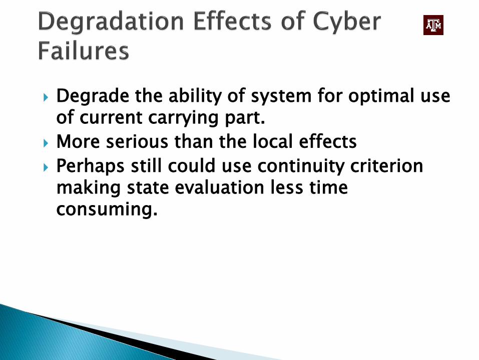
Degrade the ability of system for optimal use of current carrying part.
More serious than the local effects Perhaps still could use continuity criterion
making state evaluation less time consuming.

33© 2017 M. Sadegh Modarresi

Creating Spinning Reserve in Day Ahead Market
Using In Ground Swimming Pools

Through conventional power plants scheduling◦ Advantage: Almost a firm capacity◦ Disadvantage: Deliverability Constraint on the unit capacity
By using the flexibility of the demand itself◦ Advantage: Geographical diversity◦ Disadvantage: How much is firm capacity? Customer’s comfort
35© 2017 M. Sadegh Modarresi

© 2017 M. Sadegh Modarresi 36
Flexibility Through Residential Demand
Why swimming pool pumps was chosen by us?
Comfort Privacy Comfort Privacy

37
1-2 kW Per Pump
4-14 Hours Daily
≈1 Million pool pumps in TX
≈1.5 GW flexible capacity
10-20
=
Capacity They Can Provide:
© 2017 M. Sadegh Modarresi

38
Benefits for the Customers:
Time is important for everyone. The optimal hours a pool needs to
be filtered changes daily as a function of: Weather temperature Usage of the pool Sunlight
Giving up the control will enhance the comfort of pool owners.
© 2017 M. Sadegh Modarresi

39
Benefits for the Aggregator:
Providing a part of their ancillary service mandate using pools.
Potentially participate in the spinning reserve market.
Energy arbitrage. Capital investment? Benefits
gained from this investment?
© 2017 M. Sadegh Modarresi

Aggregator
Customers
ISO
© 2017 M. Sadegh Modarresi 40
© 2017 M. Sadegh Modarresi 41
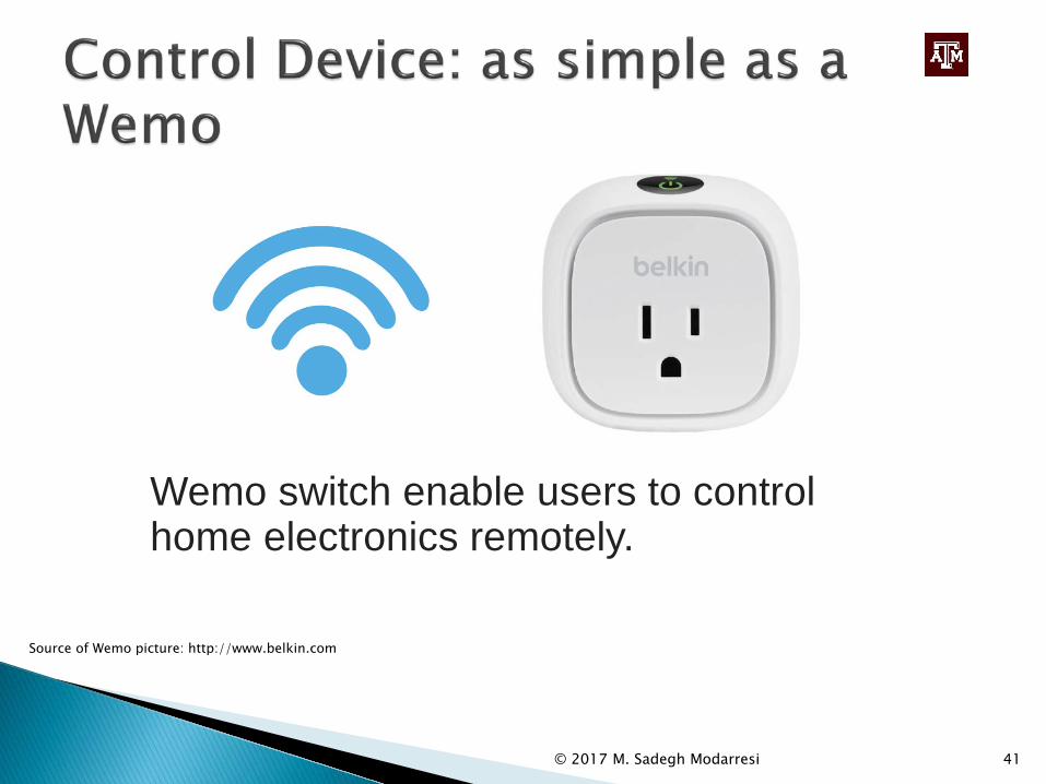
Source of Wemo picture: http://www.belkin.com
Wemo switch enable users to control home electronics remotely.

42
Communication Between the IoTSwitch and the Control Center
Control CenterCommunication links
Communication links
Communication links
© 2017 M. Sadegh Modarresi
1
ISISPP1ISP1
ISISPP1ISP N
Customer 1
Customer k1
Customer 1
Customer kN
Source of image: M. S. Modarresi, L. Xie, and C. Singh “Reserves from Controllable Swimming Pool Pumps: Reliability Assessment and Operational Planning,” in 51st Hawaii International Conference on System Sciences (HICSS), January 2018.

43
State Space Diagram of Switch and WiFi
© 2017 M. Sadegh Modarresi
Wifi up
Switch up
Wifi up
Switch down
Wifi down
Switch up
Wifi down
Switch down
λs
µs
λs
µs
λwµw λwµw
Mode A
Mode B
Source of image: M. S. Modarresi, L. Xie, and C. Singh “Reserves from Controllable Swimming Pool Pumps: Reliability Assessment and Operational Planning,” in 51st Hawaii International Conference on System Sciences (HICSS), January 2018.
• Where 𝝀𝝀𝒔𝒔 𝒂𝒂𝒂𝒂𝒂𝒂 𝝀𝝀𝒘𝒘 are failure rates of switch and WiFi respectively,
• 𝝁𝝁𝒔𝒔 𝒂𝒂𝒂𝒂𝒂𝒂 𝝁𝝁𝒘𝒘 are repair rate of the switch and WiFi network respectively
• Mode A is the state that we have access to the pump
• Mode B is the states that we do not have access to the pump

44
Probability distribution of ksuccess Each pool is accessible
(controllable) with probability 𝑷𝑷𝑴𝑴𝑴𝑴𝒂𝒂𝑴𝑴𝑴𝑴 and not controllable with (1-𝑷𝑷𝑴𝑴𝑴𝑴𝒂𝒂𝑴𝑴𝑴𝑴)
We can use Binomial distribution for k success
© 2017 M. Sadegh Modarresi
1 Customer 1
Customer g1
Customer 1
Customer gN

45
Probability Distribution of kSuccesses
© 2017 M. Sadegh Modarresi
1 Customer 1
Customer g1
Customer 1
Customer gN

© 2017 M. Sadegh Modarresi 46
Firm capacity depends on◦ Number of pools, 𝑵𝑵𝒑𝒑𝑴𝑴𝑴𝑴𝒑𝒑𝒔𝒔◦ Reliability parameters of the system◦ Threshold requirement of ISO◦ In ERCOT, Final output of the loads in 10 minutes
must be between 95% and 150% of the set-point to not-to-be punished by the market
◦ For a large number of pools, it can be shown that firm capacity can be calculated as
◦ Where D is the degrading factor

Stronger interaction between cyber and physical part and analysis is more complex.
In some situations the problem could be simplified by analyzing the cyber part and representing this through a relationship matrix.

The concepts and approaches will be explained using an example of a substation.
The problems, however, extend across the entire grid.

3 8
4 6
5 7
1
2
9
10
MU4
MU5
MU6
MU7
MU3 MU8
MU1
MU2
MU9
MU10
Process Bus
Prot. IEDProt. IEDProt. IEDProt. IED
ESProt. IEDProt. IEDProt. IEDProt. IED
ESProt. IEDProt. IEDProt. IEDProt. IED
ESBrkr. IEDBrkr. IEDBrkr. IEDBrkr. IED
ES
Line Protection
Transformer Protection
BusProtection
Breaker Control
230 KV Bus
69 KV Bus
A
B
C
D
E
F
G
H
I
J
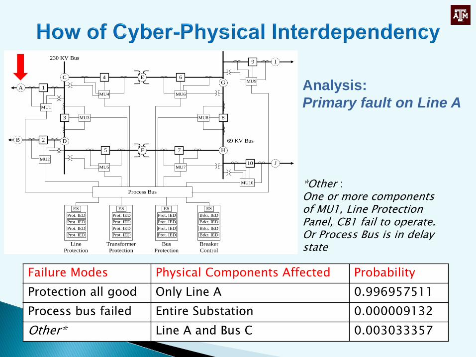
An IEC 61850 based protection system for a 230-69 kV substation
Physical Components (Power-Carrying Components):Transmission LinesPower TransformersCircuit BreakersBuses
Cyber Components:CTs/PTsMerging UnitsProcess BusEthernet SwitchesProtection IEDs
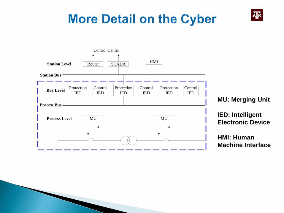
MU: Merging Unit
IED: Intelligent Electronic Device
HMI: Human Machine Interface
Control IED
Protection IED
Protection IED
Control IED
Protection IED
Control IED
MU MU
Router HMI
Control Center
Process Level
Bay Level
Station Level
Process Bus
Station Bus
SCADA

3 8
4 6
5 7
1
2
9
10
MU4
MU5
MU6
MU7
MU3 MU8
MU1
MU2
MU9
MU10
Process Bus
Prot. IEDProt. IEDProt. IEDProt. IED
ESProt. IEDProt. IEDProt. IEDProt. IED
ESProt. IEDProt. IEDProt. IEDProt. IED
ESBrkr. IEDBrkr. IEDBrkr. IEDBrkr. IED
ES
Line Protection
Transformer Protection
BusProtection
Breaker Control
230 KV Bus
69 KV Bus
A
B
C
D
E
F
G
H
I
J
Type FaultLocations
Associated Circuit Breakers
Line A Breaker 1B Breaker 2I Breaker 9J Breaker 10
Transformer E Breakers 4, 6
F Breakers 5, 7Bus C Breakers 1, 3, 4
D Breakers 2, 3, 5G Breakers 6, 8, 9H Breakers 7, 8, 10
3 8
4 6
5 7
1
2
9
10
MU4
MU5
MU6
MU7
MU3 MU8
MU1
MU2
MU9
MU10
Process Bus
Prot. IEDProt. IEDProt. IEDProt. IED
ESProt. IEDProt. IEDProt. IEDProt. IED
ESProt. IEDProt. IEDProt. IEDProt. IED
ESBrkr. IEDBrkr. IEDBrkr. IEDBrkr. IED
ES
Line Protection
Transformer Protection
BusProtection
Breaker Control
230 KV Bus
69 KV Bus
A
B
C
D
E
F
G
H
I
J
Analysis:Primary fault on Line A
Failure Modes Physical Components Affected ProbabilityProtection all good Only Line A 0.996957511Process bus failed Entire Substation 0.000009132Other* Line A and Bus C 0.003033357
*Other :One or more components of MU1, Line Protection Panel, CB1 fail to operate. Or Process Bus is in delay state
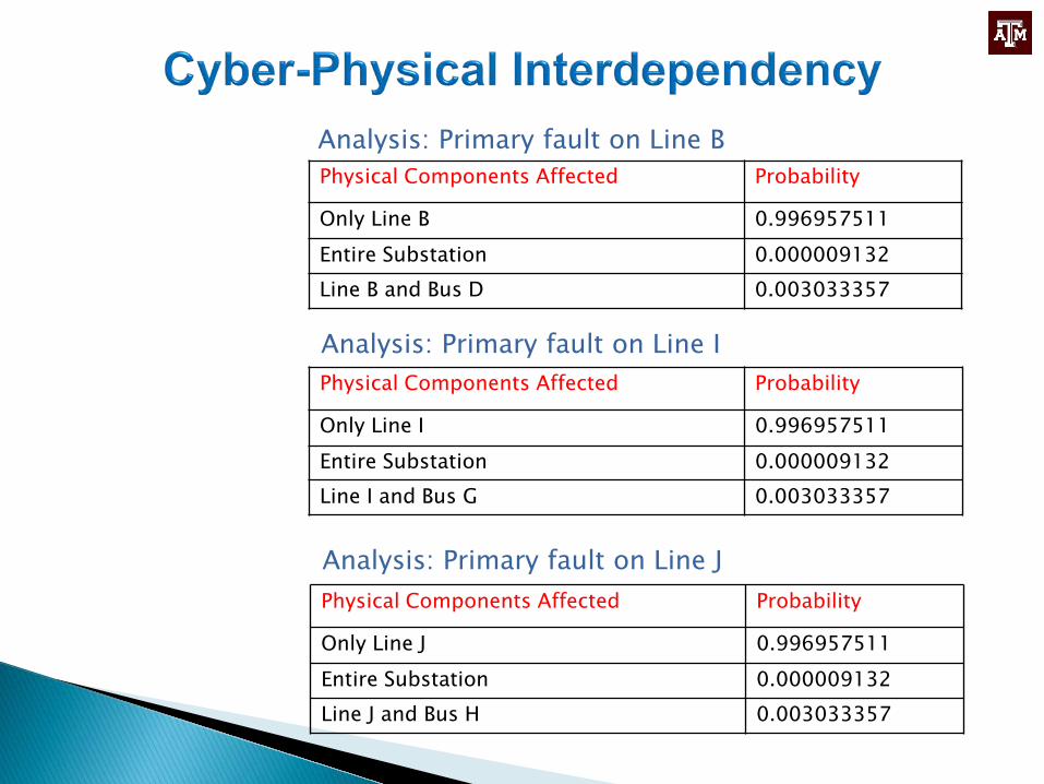
Analysis: Primary fault on Line BPhysical Components Affected Probability
Only Line B 0.996957511Entire Substation 0.000009132Line B and Bus D 0.003033357
Analysis: Primary fault on Line IPhysical Components Affected Probability
Only Line I 0.996957511Entire Substation 0.000009132Line I and Bus G 0.003033357
Analysis: Primary fault on Line JPhysical Components Affected Probability
Only Line J 0.996957511Entire Substation 0.000009132Line J and Bus H 0.003033357

3 8
4 6
5 7
1
2
9
10
MU4
MU5
MU6
MU7
MU3 MU8
MU1
MU2
MU9
MU10
Process Bus
Prot. IEDProt. IEDProt. IEDProt. IED
ESProt. IEDProt. IEDProt. IEDProt. IED
ESProt. IEDProt. IEDProt. IEDProt. IED
ESBrkr. IEDBrkr. IEDBrkr. IEDBrkr. IED
ES
Line Protection
Transformer Protection
BusProtection
Breaker Control
230 KV Bus
69 KV Bus
A
B
C
D
E
F
G
H
I
J
Analysis:Primary fault on Transformer E
PhysicalComponents Affected
Probability
Only E 0.996942336
EntireSubstation
0.000009132
E and C 0.000015174
E and G 0.000015174
E, C, and G 0.003018182

3 8
4 6
5 7
1
2
9
10
MU4
MU5
MU6
MU7
MU3 MU8
MU1
MU2
MU9
MU10
Process Bus
Prot. IEDProt. IEDProt. IEDProt. IED
ESProt. IEDProt. IEDProt. IEDProt. IED
ESProt. IEDProt. IEDProt. IEDProt. IED
ESBrkr. IEDBrkr. IEDBrkr. IEDBrkr. IED
ES
Line Protection
Transformer Protection
BusProtection
Breaker Control
230 KV Bus
69 KV Bus
A
B
C
D
E
F
G
H
I
J
Analysis:Primary fault on Bus C
PhysicalComponents Affected
Probability
Only C 0.996927163
EntireSubstation
0.000009132
A and C 0.000015174
C and D 0.000015174
C and E 0.000015174
A, C, and D 2.31*10-10
A, C, and E 2.31*10-10
C, D, and E 2.31*10-10
A, C, D, and E 0.003018182

Cyber-Physical Interface Matrix (CPIM)
Line A 0.9969575 0.0000091 0.0030334 0 ……Line B 0.9969575 0.0000091 0.0030334 0 ……Line I 0.9969575 0.0000091 0.0030334 0 ………… …… …… …… …… ……
Bus H 0.9969272 0.0000091 0.0000152 0.0000152 ……
Representing Interdependency for Reliability Analysis
Line A Event-1 Event-2 Event-3 Event-4
Line BLine I…… …… …… …… …… ……
Bus H
Consequent Events Matrix (CEM)

Composite system reliability evaluation with the use of cyber-physical interface matrix
3 8
4 6
5 7
1
2
9
10
MU4
MU5
MU6
MU7
MU3 MU8
MU1
MU2
MU9
MU10
Process Bus
Prot. IEDProt. IEDProt. IEDProt. IED
ESProt. IEDProt. IEDProt. IEDProt. IED
ESProt. IEDProt. IEDProt. IEDProt. IED
ESBrkr. IEDBrkr. IEDBrkr. IEDBrkr. IED
ES
Line Protection
Transformer Protection
BusProtection
Breaker Control
230 KV Bus
69 KV Bus
A
B
C
D
E
F
G
H
I
J
230 KV Bus
69 KV Bus
AE
FB
C
D
G
H
I
J
G1
G2
G3
G4
K
L
M
N
O
P
Q
R
Physical Part
Cyber Part

Composite system reliability evaluation with the use of cyber-physical interface matrix
230 KV Bus
69 KV Bus
AE
FB
C
D
G
H
I
J
G1
G2
G3
G4
K
L
M
N
O
P
Q
R
Step 1: Set the initial state of all components as UP and set the simulation time t = 0.
Step 2: For each individual component, draw a random decimal number zi between 0 and 1 to compute the time to the next event.
𝑻𝑻𝒊𝒊 = −𝒑𝒑𝒂𝒂(𝒛𝒛𝒊𝒊)𝝆𝝆𝒊𝒊
Depending on whether the ith component is UP or DOWN, λi or µi is used in place of ρi
Composite system reliability evaluation with the use of cyber-physical interface matrix
230 KV Bus
69 KV Bus
AE
FB
C
D
G
H
I
J
G1
G2
G3
G4
K
L
M
N
O
P
Q
R
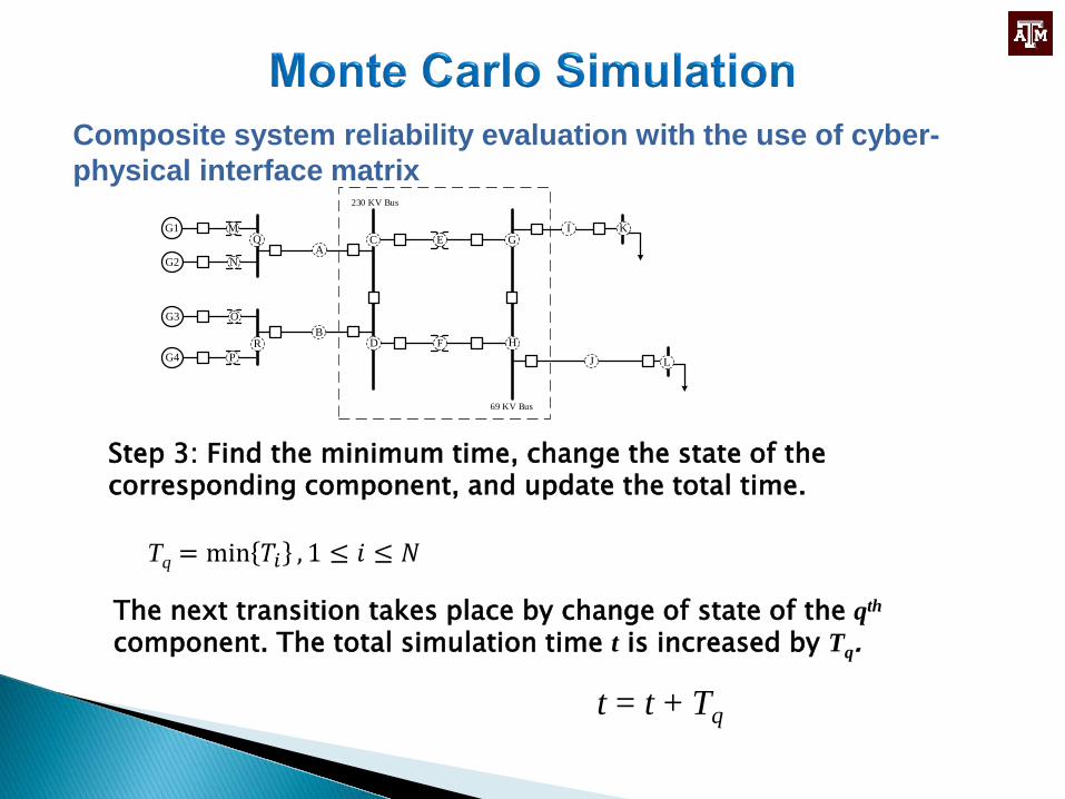
Step 3: Find the minimum time, change the state of the corresponding component, and update the total time.
The next transition takes place by change of state of the qth
component. The total simulation time t is increased by Tq.
Tq = min 𝑇𝑇𝑖𝑖 , 1 ≤ 𝑖𝑖 ≤ 𝑁𝑁
t = t + Tq

Composite system reliability evaluation with the use of cyber-physical interface matrix
230 KV Bus
69 KV Bus
AE
FB
C
D
G
H
I
J
G1
G2
G3
G4
K
L
M
N
O
P
Q
R
Step 4: Change the qth component’s state accordingly. For each component i
𝑇𝑇𝑖𝑖 = 𝑇𝑇𝑖𝑖 − Tq

Composite system reliability evaluation with the use of cyber-physical interface matrix
230 KV Bus
69 KV Bus
AE
FB
C
D
G
H
I
J
G1
G2
G3
G4
K
L
M
N
O
P
Q
R
Step 5: If the state of the qth component transits from UP to DOWN, which means a primary fault occurs on this component, then the cyber-physical interface matrix is used to determine if there are some subsequent failures causing more components out of service due to the cyber part’s malfunction.

Composite system reliability evaluation with the use of cyber-physical interface matrix
230 KV Bus
69 KV Bus
AE
FB
C
D
G
H
I
J
G1
G2
G3
G4
K
L
M
N
O
P
Q
R
Line A 0.9969575 0.0000091 0.0030334 0 ………… …… …… …… …… ……
Transformer E 0.9969423 0.0000091 0.0000152 0.0000152 ……
…… …… …… …… …… ……Bus H 0.9969272 0.0000091 0.0000152 0.0000152 ……
Draw another random decimal number y (0 < y ≤ 1)

Composite system reliability evaluation with the use of cyber-physical interface matrix
230 KV Bus
69 KV Bus
AE
FB
C
D
G
H
I
J
G1
G2
G3
G4
K
L
M
N
O
P
Q
R
𝑇𝑇𝑖𝑖 = −𝑙𝑙𝑛𝑛(𝑧𝑧𝑖𝑖)𝜌𝜌𝑖𝑖
For Transformer E, use µi in place of ρi
For Bus C, use µi,exp in place of ρi
µi,exp is an expedited repair rate, called switching rate
How to determine the next transition time of Transformer E and Bus C?

Composite system reliability evaluation with the use of cyber-physical interface matrix
230 KV Bus
69 KV Bus
AE
FB
C
D
G
H
I
J
G1
G2
G3
G4
K
L
M
N
O
P
Q
R
Step 6: Perform a network power flow analysis to assess system operation states. Update system-wide reliability indices.
Repeat steps 3–6 until convergence is achieved.

Composite system reliability evaluation with the use of cyber-physical interface matrix
230 KV Bus
69 KV Bus
AE
FB
C
D
G
H
I
J
G1
G2
G3
G4
K
L
M
N
O
P
Q
R
When the simulation finishes, system-wide reliability indices can be obtained.
𝐿𝐿𝐿𝐿𝐿𝐿𝐿𝐿 = �𝑖𝑖=1
𝑁𝑁𝑠𝑠 𝐻𝐻𝑖𝑖 ∗ 𝑡𝑡𝑖𝑖𝑡𝑡𝑡𝑡𝑡𝑡𝑡𝑡𝑡𝑡𝑡𝑡
Ns Total number of iterations simulated;Hi Equals 1 if load curtailment occurs in the ith
iteration; otherwise it equals 0; ti Simulated time in the ith iteration, with the
unit of year;ttotal Total simulated time, with the unit of year.Ri Load curtailment during the ith iteration,
with the unit of MW;
𝐸𝐸𝐸𝐸𝑁𝑁𝐸𝐸 = �𝑖𝑖=1
𝑁𝑁𝑠𝑠 𝑅𝑅𝑖𝑖 ∗ 𝑡𝑡𝑖𝑖 ∗ 8760𝑡𝑡𝑡𝑡𝑡𝑡𝑡𝑡𝑡𝑡𝑡𝑡
𝐿𝐿𝐿𝐿𝐿𝐿𝐸𝐸 = 𝐿𝐿𝐿𝐿𝐿𝐿𝐿𝐿 ∗ 8760(With the unit of hours/year )
(With the unit of MWh/year )

~
~
4
85 MW
20 MW
20 MW
40 MW
20 MW
~
~
~
~
~
~
~
~
~
LoadBus 3
LoadBus 4
LoadBus 5
LoadBus 6
GeneratingStation 1 Generating
Station 2
G1
G3
G2
G4
G5 G6
G7
G8
G9
G10
G11
1 2
3
6
5 8
7
9
The size of this system is small to permit reasonable time for extension of cyber part and development of interface matrices.But the configuration of this system is sufficiently detailed to reflect the actual features of a practical system
RBTS Test System
Illustrating the overall methodology on a standard test system
Buses 3–5 are extended with cyber configurations

~
~
4
85 MW
20 MW
20 MW
40 MW
20 MW
~
~
~
~
~
~
~
~
~
LoadBus 3
LoadBus 4
LoadBus 5
LoadBus 6
GeneratingStation 1 Generating
Station 2
G1
G3
G2
G4
G5 G6
G7
G8
G9
G10
G11
1 2
3
6
5 8
7
9
3-1
MU3-1
3-2 3-3
3-4 3-5
MU3-2
MU3-3
MU3-4
MU3-5
MU3-6
MU3-7
MU3-8
MU3-9
Process Bus
Line 1Protection
Panel
Line 4Protection
Panel
Line 5Protection
Panel
Line 6Protection
Panel
Line 6 Line 5 Line 4 Line 1
Load 3
Extend bus 3 of the RBTS Test System with substation protection configurations.
Physical part of the RBTS Extension with cyber part in Bus 3

~
~
4
85 MW
20 MW
20 MW
40 MW
20 MW
~
~
~
~
~
~
~
~
~
LoadBus 3
LoadBus 4
LoadBus 5
LoadBus 6
GeneratingStation 1 Generating
Station 2
G1
G3
G2
G4
G5 G6
G7
G8
G9
G10
G11
1 2
3
6
5 8
7
9
Extend bus 4 of the RBTS with substation protection configurations.
Physical part of the RBTS Extension with cyber part in Bus 4
4-1
MU4-1
4-2 4-3
4-4 4-5
MU4-2
MU4-3
MU4-4
MU4-5
MU4-6
MU4-7
MU4-8
MU4-9
Process Bus
Line 2Protection
Panel
Line 4Protection
Panel
Line 7Protection
Panel
Line 8Protection
Panel
Line 2 Line 8 Line 4 Line 7
Load 4

~
~
4
85 MW
20 MW
20 MW
40 MW
20 MW
~
~
~
~
~
~
~
~
~
LoadBus 3
LoadBus 4
LoadBus 5
LoadBus 6
GeneratingStation 1 Generating
Station 2
G1
G3
G2
G4
G5 G6
G7
G8
G9
G10
G11
1 2
3
6
5 8
7
9
Extend bus 5 of the RBTS with substation protection configurations.
Physical part of the RBTS Extension with cyber part in Bus 5
5-1
MU5-1
5-2
5-3 5-4
MU5-2
MU5-3
MU5-4
MU5-5
MU5-6
Process Bus
Line 5Protection
Panel
Line 8Protection
Panel
Line 9Protection
Panel
Line 5 Line 8Load 5
Line 9
MU5-7

~
~
4
85 MW
20 MW
20 MW
40 MW
20 MW
~
~
~
~
~
~
~
~
~
LoadBus 3
LoadBus 4
LoadBus 5
LoadBus 6
GeneratingStation 1 Generating
Station 2
G1
G3
G2
G4
G5 G6
G7
G8
G9
G10
G11
1 2
3
6
5 8
7
9
Generation Variation
Physical part of the RBTS
Unit No.
Bus
Rating (MW)
Failure Rate ( /year)
MRT (hours)
1 1 40 6.0 452 1 40 6.0 453 1 10 4.0 454 1 20 5.0 455 2 5 2.0 456 2 5 2.0 457 2 40 3.0 608 2 20 2.4 559 2 20 2.4 5510 2 20 2.4 5511 2 20 2.4 55
Load VariationThe hourly load profile is created based on the information in Tables 1, 2, and 3 of the IEEE Reliability Test System*.
*IEEE Committee Report, “IEEE reliability test system,” IEEE Trans. Power App. and Syst., vol. PAS-98, no. 6, pp. 2047–2054, Nov./Dec. 1979.

3-1
MU3-1
3-2 3-3
3-4 3-5
MU3-2
MU3-3
MU3-4
MU3-5
MU3-6
MU3-7
MU3-8
MU3-9
Process Bus
Line 1Protection
Panel
Line 4Protection
Panel
Line 5Protection
Panel
Line 6Protection
Panel
Line 6 Line 5 Line 4 Line 1
Load 3
Analyze the cyber failure modes and consequent events and obtain the Cyber-Physical Interface Matrices (CPIM) for Buses 3-5.
𝑝𝑝1,1 𝑝𝑝1,2𝑝𝑝2,1 𝑝𝑝2,2
⋯𝑝𝑝1,𝑛𝑛𝑝𝑝2,𝑛𝑛
⋮ ⋱ ⋮𝑝𝑝𝑚𝑚,1 𝑝𝑝𝑚𝑚,2 ⋯ 𝑝𝑝𝑚𝑚,𝑛𝑛

Results: The CPIM and CEM of Bus 3
Fault Location Probabilities
Line 1 0.996899850569 0.000009132337 0.000027312491 0.000027312491 0.003036392112Line 4 0.996899850569 0.000009132337 0.000027312491 0.000027312491 0.003036392112Line 5 0.996899850569 0.000009132337 0.000027312491 0.000027312491 0.003036392112Line 6 0.996899850569 0.000009132337 0.000027312491 0.000027312491 0.003036392112
Fault Location Events
Line 1 100000000000 100111000000 100100000000 100000000100 100100000100Line 4 000100000000 100111000000 000110000000 100100000000 100110000000Line 5 000010000000 100111000000 000011000000 000110000000 000111000000Line 6 000001000000 100111000000 000001000100 000011000000 000011000100
The Cyber-Physical Interface Matrix (CPIM) of Bus 3
The Consequent Event Matrix (CEM) of Bus 3

Results: The CPIM and CEM of Bus 4
The Cyber-Physical Interface Matrix (CPIM) of Bus 4
The Consequent Event Matrix (CEM) of Bus 4
Fault Location Probabilities
Line 2 0.996899850569 0.000009132337 0.000027312491 0.000027312491 0.003036392112Line 4 0.996899850569 0.000009132337 0.000027312491 0.000027312491 0.003036392112Line 7 0.996899850569 0.000009132337 0.000027312491 0.000027312491 0.003036392112Line 8 0.996899850569 0.000009132337 0.000027312491 0.000027312491 0.003036392112
Fault Location Events
Line 2 010000000000 010100110000 010000000010 010000010000 010000010010Line 4 000100000000 010100110000 000100010000 000100100000 000100110000Line 7 000000100000 010100110000 000100100000 000000100010 000100100010Line 8 000000010000 010100110000 010000010000 000100010000 010100010000
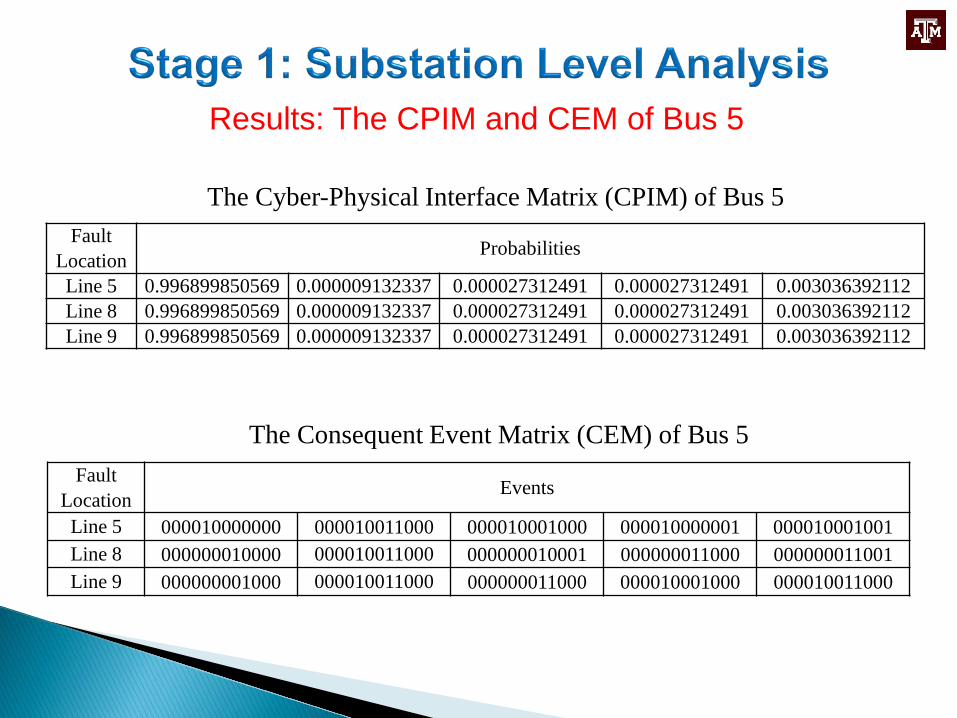
Results: The CPIM and CEM of Bus 5
The Cyber-Physical Interface Matrix (CPIM) of Bus 5
The Consequent Event Matrix (CEM) of Bus 5
Fault Location Probabilities
Line 5 0.996899850569 0.000009132337 0.000027312491 0.000027312491 0.003036392112Line 8 0.996899850569 0.000009132337 0.000027312491 0.000027312491 0.003036392112Line 9 0.996899850569 0.000009132337 0.000027312491 0.000027312491 0.003036392112
Fault Location Events
Line 5 000010000000 000010011000 000010001000 000010000001 000010001001Line 8 000000010000 000010011000 000000010001 000000011000 000000011001Line 9 000000001000 000010011000 000000011000 000010001000 000010011000

~
~
4
85 MW
20 MW
20 MW
40 MW
20 MW
~
~
~
~
~
~
~
~
~
LoadBus 3
LoadBus 4
LoadBus 5
LoadBus 6
GeneratingStation 1 Generating
Station 2
G1
G3
G2
G4
G5 G6
G7
G8
G9
G10
G11
1 2
3
6
5 8
7
9
Utilize the results of the interface matrices, perform a Monte-Carlo simulation for the composite system, and obtain numerical results of system-wide reliability indices.

~
~
4
85 MW
20 MW
20 MW
40 MW
20 MW
~
~
~
~
~
~
~
~
~
LoadBus 3
LoadBus 4
LoadBus 5
LoadBus 6
GeneratingStation 1 Generating
Station 2
G1
G3
G2
G4
G5 G6
G7
G8
G9
G10
G11
1 2
3
6
5 8
7
9
Objective: 𝑦𝑦 = 𝑀𝑀𝑖𝑖𝑛𝑛∑𝑖𝑖=1𝑁𝑁𝑏𝑏 𝐶𝐶𝑖𝑖
subject to:
�𝐵𝐵𝜃𝜃 + 𝐺𝐺 + 𝐶𝐶 = 𝐿𝐿𝐺𝐺 ≤ 𝐺𝐺𝑚𝑚𝑡𝑡𝑚𝑚
𝐶𝐶 ≤ 𝐿𝐿𝐷𝐷𝐷𝐷𝜃𝜃 ≤ 𝐹𝐹𝑚𝑚𝑡𝑡𝑚𝑚
−𝐷𝐷𝐷𝐷𝜃𝜃 ≤ 𝐹𝐹𝑚𝑚𝑡𝑡𝑚𝑚
𝐺𝐺,𝐶𝐶 ≥ 0𝜃𝜃1 = 0𝜃𝜃2…𝑁𝑁𝑏𝑏 unrestricted
Nb Number of busesC 𝑁𝑁𝑏𝑏 × 1 vector of bus load
curtailmentsCi Load curtailment at bus i�𝐵𝐵 𝑁𝑁𝑏𝑏 × 𝑁𝑁𝑏𝑏 augmented node
susceptance matrixG 𝑁𝑁𝑏𝑏 × 1 vector of bus actual
generating powerGmax 𝑁𝑁𝑏𝑏 × 1 vector of bus
maximum generating availability
L 𝑁𝑁𝑏𝑏 × 1 vector of bus loadsD 𝑁𝑁𝑡𝑡 × 𝑁𝑁𝑡𝑡 diagonal matrix of
transmission line susceptances, with Nt the number of transmission lines
A 𝑁𝑁𝑡𝑡 × 𝑁𝑁𝑏𝑏 line-bus incidence matrix
θ 𝑁𝑁𝑏𝑏 × 1 vector of bus voltage angles
Fmax 𝑁𝑁𝑡𝑡 × 1 vector of transmission line power flow capacities
Variables: θ, G, and C
Total number of variables: 3Nb

Brief Results
EENS (MWh/year)Δ
If protection systems are perfectly reliable Considering protection malfunctions
Bus 1 0 0 N/ABus 2 1.862 2.655 42.59%Bus 3 2.828 8.597 204.00%Bus 4 1.950 10.095 417.69%Bus 5 2.145 3.729 73.85%Bus 6 103.947 116.104 11.70%
Overall System 112.732 141.180 25.24%
Impact on Expected Energy Not Served (EENS)

G1
G4
MU1-1
MU1-3
MU1-2
ES 1-1 ES 1-2
ES 1-3
S1-L5
MU2-1
MU2-2
MU2-3
ES 2-1 ES 2-2
ES 2-3
S2-L6
Line 5
Line 2
Line 1
Line 6
Line 3
Line 4
Line 7Line 8
S1-L1 S1-L2 S2-L3 S2-L1
Bus 1 Bus 2
Bus 3 Bus 4
MU3-2
MU3-1
MU3-3
ES 3-1 ES 3-2
ES 3-3
S3-L4 S3-L7 S3-L2
MU4-2
MU4-1
MU4-3
ES 4-1 ES 4-2
ES 4-3
S4-L3 S4-L8 S4-L4

Two types of cyber link failures:(a) A link is unavailable
due to packet delay resulting from traffic congestion or queue failure;
(b) A link is physically damaged.
Failure type (b) is relatively rare and thus only failure type (a) is considered in this research
G1
G4
MU1-1
MU1-3
MU1-2
ES 1-1 ES 1-2
ES 1-3
S1-L5
MU2-1
MU2-2
MU2-3
ES 2-1 ES 2-2
ES 2-3
S2-L6
Line 5
Line 2
Line 1
Line 6
Line 3
Line 4
Line 7Line 8
S1-L1 S1-L2 S2-L3 S2-L1
Bus 1 Bus 2
Bus 3 Bus 4
MU3-2
MU3-1
MU3-3
ES 3-1 ES 3-2
ES 3-3
S3-L4 S3-L7 S3-L2
MU4-2
MU4-1
MU4-3
ES 4-1 ES 4-2
ES 4-3
S4-L3 S4-L8 S4-L4
MU1-1
MU1-3
MU1-2ES 1-1 ES 1-2
ES 1-3
S1-L5 S1-L1 S1-L2
1
2
34
5
67
8 9
1011
12
13
14
15
16
17
1819
20
21
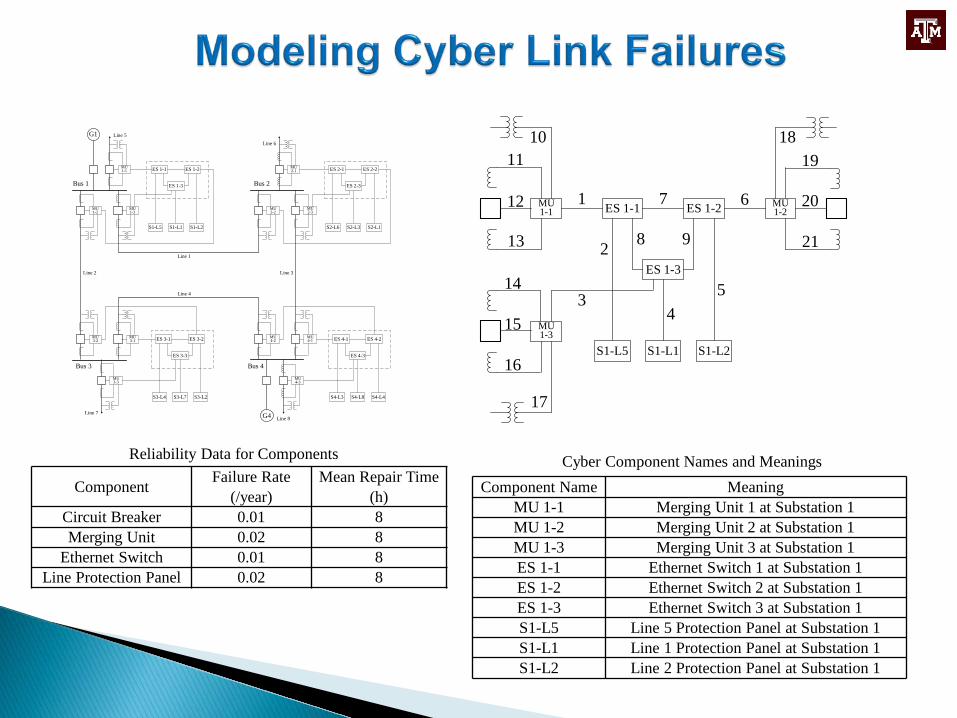
Component Name MeaningMU 1-1 Merging Unit 1 at Substation 1MU 1-2 Merging Unit 2 at Substation 1MU 1-3 Merging Unit 3 at Substation 1ES 1-1 Ethernet Switch 1 at Substation 1ES 1-2 Ethernet Switch 2 at Substation 1ES 1-3 Ethernet Switch 3 at Substation 1S1-L5 Line 5 Protection Panel at Substation 1S1-L1 Line 1 Protection Panel at Substation 1S1-L2 Line 2 Protection Panel at Substation 1
Component Failure Rate (/year)
Mean Repair Time (h)
Circuit Breaker 0.01 8Merging Unit 0.02 8
Ethernet Switch 0.01 8Line Protection Panel 0.02 8
Cyber Component Names and MeaningsReliability Data for Components
MU1-1
MU1-3
MU1-2ES 1-1 ES 1-2
ES 1-3
S1-L5 S1-L1 S1-L2
1
2
34
5
67
8 9
1011
12
13
14
15
16
17
1819
20
21
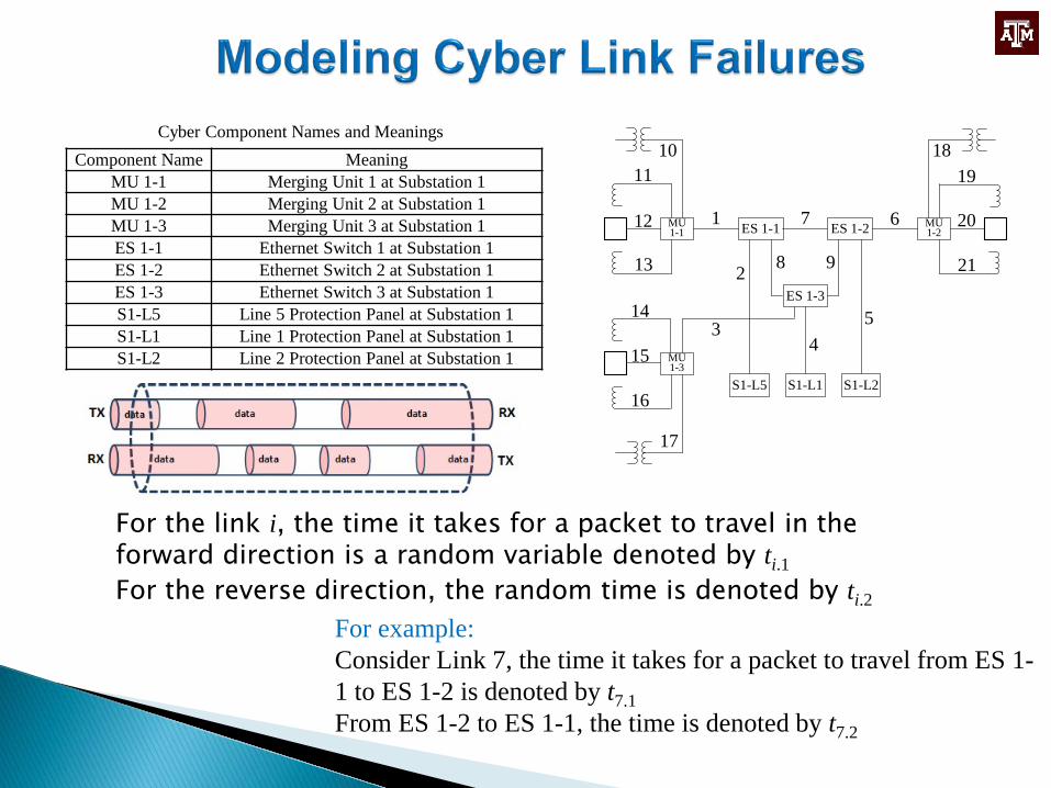
Component Name MeaningMU 1-1 Merging Unit 1 at Substation 1MU 1-2 Merging Unit 2 at Substation 1MU 1-3 Merging Unit 3 at Substation 1ES 1-1 Ethernet Switch 1 at Substation 1ES 1-2 Ethernet Switch 2 at Substation 1ES 1-3 Ethernet Switch 3 at Substation 1S1-L5 Line 5 Protection Panel at Substation 1S1-L1 Line 1 Protection Panel at Substation 1S1-L2 Line 2 Protection Panel at Substation 1
Cyber Component Names and Meanings
For the link i, the time it takes for a packet to travel in the forward direction is a random variable denoted by ti.1For the reverse direction, the random time is denoted by ti.2
For example:Consider Link 7, the time it takes for a packet to travel from ES 1-1 to ES 1-2 is denoted by t7.1From ES 1-2 to ES 1-1, the time is denoted by t7.2

MU1-1
MU1-3
MU1-2ES 1-1 ES 1-2
ES 1-3
S1-L5 S1-L1 S1-L2
1
2
34
5
67
8 9
1011
12
13
14
15
16
17
1819
20
21
Component Name MeaningMU 1-1 Merging Unit 1 at Substation 1MU 1-2 Merging Unit 2 at Substation 1MU 1-3 Merging Unit 3 at Substation 1ES 1-1 Ethernet Switch 1 at Substation 1ES 1-2 Ethernet Switch 2 at Substation 1ES 1-3 Ethernet Switch 3 at Substation 1S1-L5 Line 5 Protection Panel at Substation 1S1-L1 Line 1 Protection Panel at Substation 1S1-L2 Line 2 Protection Panel at Substation 1
Cyber Component Names and Meanings
Consider the communication from MU 1-1 to S1-L1. There are two possible paths: 1-8-4 and 1-7-9-4.
𝑝𝑝𝑓𝑓𝑡𝑡𝑖𝑖𝑡𝑡 = Pr[ 𝑡𝑡1.1 + 𝑡𝑡8.1 + 𝑡𝑡4.1 > 𝑇𝑇𝑡𝑡𝑡𝑡𝑡𝑡 𝑎𝑎𝑛𝑛𝑎𝑎 (𝑡𝑡1.1 + 𝑡𝑡7.1 + 𝑡𝑡9.1 + 𝑡𝑡4.1 > 𝑇𝑇𝑡𝑡𝑡𝑡𝑡𝑡)]
where Ttsd is a predefined threshold delay value for the two paths.

MU1-1
MU1-3
MU1-2ES 1-1 ES 1-2
ES 1-3
S1-L5 S1-L1 S1-L2
1
2
34
5
67
8 9
1011
12
13
14
15
16
17
1819
20
21 𝑝𝑝𝑓𝑓𝑡𝑡𝑖𝑖𝑡𝑡= Pr[ 𝑡𝑡1.1 + 𝑡𝑡8.1 + 𝑡𝑡4.1 > 𝑇𝑇𝑡𝑡𝑡𝑡𝑡𝑡 𝑎𝑎𝑛𝑛𝑎𝑎 (𝑡𝑡1.1 + 𝑡𝑡7.1+ 𝑡𝑡9.1 + 𝑡𝑡4.1 > 𝑇𝑇𝑡𝑡𝑡𝑡𝑡𝑡)]
Similarly, with any two components specified as the two ends of a communication path, the path failure probability can be computed from the cyber link level parameters
From MU 1-1 to S1-L1

MU1-1
MU1-3
MU1-2ES 1-1 ES 1-2
ES 1-3
S1-L5 S1-L1 S1-L2
1
2
34
5
67
8 9
1011
12
13
14
15
16
17
1819
20
21The detailed procedures are based on queueing theory and are beyond the scope of this research. These probabilities can be assumed directly at the path level.
From To Forward Path Failure Probability Reverse Path Failure ProbabilityMU 1-1 S1-L5 0.002 0.002MU 1-1 S1-L1 0.001 0.001MU 1-1 S1-L2 0.001 0.001MU 1-2 S1-L5 0.001 0.001MU 1-2 S1-L1 0.001 0.001MU 1-2 S1-L2 0.002 0.002MU 1-3 S1-L5 0.001 0.001MU 1-3 S1-L1 0.002 0.002MU 1-3 S1-L2 0.001 0.001

G1
G4
MU1-1
MU1-3
MU1-2
ES 1-1 ES 1-2
ES 1-3
S1-L5
MU2-1
MU2-2
MU2-3
ES 2-1 ES 2-2
ES 2-3
S2-L6
Line 5
Line 2
Line 1
Line 6
Line 3
Line 4
Line 7Line 8
S1-L1 S1-L2 S2-L3 S2-L1
Bus 1 Bus 2
Bus 3 Bus 4
MU3-2
MU3-1
MU3-3
ES 3-1 ES 3-2
ES 3-3
S3-L4 S3-L7 S3-L2
MU4-2
MU4-1
MU4-3
ES 4-1 ES 4-2
ES 4-3
S4-L3 S4-L8 S4-L4
Results
Primary Fault
LocationProbabilities of Consequent Events
Line 1 0.9919152 0.0040342 0.0040342 0.0000164Line 2 0.9919152 0.0040342 0.0040342 0.0000164Line 3 0.9919152 0.0040342 0.0040342 0.0000164Line 4 0.9919152 0.0040342 0.0040342 0.0000164Line 5 0.9959494 0.0040506 0 0Line 6 0.9959494 0.0040506 0 0Line 7 0.9959494 0.0040506 0 0Line 8 0.9959494 0.0040506 0 0
The Cyber-Physical Interface Matrix
Primary Fault
LocationConsequent Events
Line 1 10000000 11001000 10100100 11101100Line 2 01000000 11001000 01010010 11011010Line 3 00100000 10100100 00110001 10110101Line 4 00010000 01010010 00110001 01110011Line 5 00001000 11001000 00000000 00000000Line 6 00000100 10100100 00000000 00000000Line 7 00000010 01010010 00000000 00000000Line 8 00000001 00110001 00000000 00000000
The Consequent Event Matrix

Stage 1: Substation Level Analysis
The results of CPIMs and CEMs can be directly utilized.Monte-Carlo simulation performed in this stage is generic and applicable for large power systems.
Analysis at this stage can be performed locally at each substation and the computations can be performed offline.
Stage 2: Composite System Level Analysis
The CPIM decouples the 2 stages of analysis, making the overall analysis more tractable.

Cyber-Physical Interactions◦ This is only starting point◦More detailed models need to be developed.◦We need to consider inter-substation interactions◦ Consider the interaction of physical on the cyber as well◦Where ever there is cyber-physical interaction there could be a potential problem.

Computational Methods◦ Generally non-sequential Monte Carlo
Simulation is preferred as a more efficient method of for reliability evaluation.◦ Several variance reduction techniques like
importance sampling have been developed to make it even faster, especially those incorporating the concept of cross-entropy.◦ The efficiency of non-sequential MCS is
based on the assumption of independence between the components, although limited dependence can be accommodated.

IEEE RTS – Reliability Test System has served as a resource for the researchers and developers to test their algorithms and compare their results with others.
Additional information about distribution has since been added.
This test system does not have information on the related cyber part.
A taskforce under the Reliability, Risk and Probability Applications Subcommittee (RRPA) is investigating adding configurations and data on the cyber part.

◦ Because of interdependence introduced by cyber part it becomes difficult to use non-sequential MC and the associated variance reduction techniques. So we have used sequential MCS.◦We have also proposed a non-sequential MCS technique to solve this problem but more work is needed in this direction.

1. C. Singh, A. Sprintson, “Reliability Assurance of Cyber-Physical Power Systems”, IEEE PES General Meeting, July 2010.
2. Yan Zhang, Alex Sprintson, and Chanan Singh, “An Integrative Approach to Reliability Analysis of an IEC 61850 Digital Substation“, IEEE PES General Meeting, July 2012.
3. H. Lei, C. Singh, and A. Sprintson, “Reliability modeling and analysis of IEC 61850 based substation protection systems,” IEEE Transactions on Smart Grid, vol. 5, no. 5, pp. 2194–2202, September 2014.
4. H. Lei and C. Singh, “Power system reliability evaluation considering cyber-malfunctions in substations,” Electric Power Systems Research, vol. 129, pp. 160-169, December 2015.
5. M. S. Modarresi, L. Xie, and C. Singh “Reserves from Controllable Swimming Pool Pumps: Reliability Assessment and Operational Planning,” in 51st Hawaii International Conference on System Sciences (HICSS), January 2018

Presenter’s email: [email protected]


