Change in trade wind inversion frequencyimplicated in the decline of an alpine plantKrushelnycky et al.

Krushelnycky et al. Climate Change Responses (2016) 3:1 DOI 10.1186/s40665-016-0015-2

Krushelnycky et al. Climate Change Responses (2016) 3:1 DOI 10.1186/s40665-016-0015-2

RESEARCH Open Access

Change in trade wind inversion frequencyimplicated in the decline of an alpine plant

Paul D. Krushelnycky1*, Forest Starr2, Kim Starr2, Ryan J. Longman3, Abby G. Frazier3, Lloyd L. Loope4,5

and Thomas W. Giambelluca3

Abstract

Background: Detailed assessments of species responses to climate change are uncommon, owing to the limitednature of most ecological and local climate data sets. Exceptions, such as the case of the Haleakalā silversword, canprovide important insights into the complexity of biological responses to changing climate conditions. We presenta time series of decadal population censuses, combined with a pair of early population projections, which togetherspan the past 80 years of demographic history for this alpine plant.

Results: The time series suggests a strong population recovery from the 1930s through the 1980s, likely owing atleast in part to management actions taken on its behalf. In contrast, the population is estimated to have suffered adecline of approximately 60 % since the early 1990s. Fine-scale estimates of rainfall within silversword habitat arestrongly correlated with these decadal-scale population changes over the past 50 years, with rainfall estimated tobe substantially lower on average during the two most recent inter-census periods (after 1991). The reversal in thesilversword population trajectory, and declines in rainfall in silversword habitat, coincide with an abrupt increase inthe frequency of occurrence of the trade wind inversion (TWI) in Hawaiʻi around 1990.

Conclusions: The shift in TWI incidence, which is linked to stronger subsidence in the Hadley circulation, has led todrier conditions in high elevation ecosystems in Hawaiʻi and appears to be eliciting ecological responses. Otherregions influenced by the TWI could be similarly affected. The silversword case study reveals additional unexpectedoutcomes, such as the likely initial retraction from wetter, rather than drier, portions of the range in response todrying conditions. This pattern may stem in part from variation in drought tolerance across the range, highlightingthe importance of detailed ecological and climatic information for making accurate predictions about climatechange responses.

Keywords: Climate change ecology, Trade wind inversion, Silversword, Alpine plants, Population declines,Argyroxyphium sandwicense

BackgroundEmpirical evidence of species response to recent climatechange is usually fragmentary, owing to a shortage oflong-term, comprehensive data sets. Range shifts areoften estimated from limited survey data, most com-monly comparing two points in time and encompassingonly a portion of a species’ range [1], and informationon changes in population size that may or may notaccompany such shifts is often lacking. At the sametime, species responses to climate change are increasingly

* Correspondence: pauldk@hawaii.edu1Department of Plant and Environmental Protection Sciences, University ofHawaiʻi at Mānoa, Honolulu, HI 96822, USAFull list of author information is available at the end of the article

© 2016 Krushelnycky et al. Open Access ThisInternational License (http://creativecommonsreproduction in any medium, provided you gthe Creative Commons license, and indicate if(http://creativecommons.org/publicdomain/ze

recognized and predicted to be more complex than simplepoleward or upslope migration [2–5], and the incompletenature of much ecological information likely hinders abetter understanding of this complexity. This may beespecially true in situations where precipitation is a keydeterminant of distributions and demographics, becausechanges to regional precipitation may be driven by com-plicated alterations to global circulation patterns com-bined with the influence of local features [6, 7], andchanges in precipitation frequently act in opposition tochanges in temperature [2, 3, 8].Analyses of response patterns among large numbers

of species in regional or global floras and faunas canbe highly insightful and help overcome some of the

article is distributed under the terms of the Creative Commons Attribution 4.0.org/licenses/by/4.0/), which permits unrestricted use, distribution, andive appropriate credit to the original author(s) and the source, provide a link tochanges were made. The Creative Commons Public Domain Dedication waiverro/1.0/) applies to the data made available in this article, unless otherwise stated.

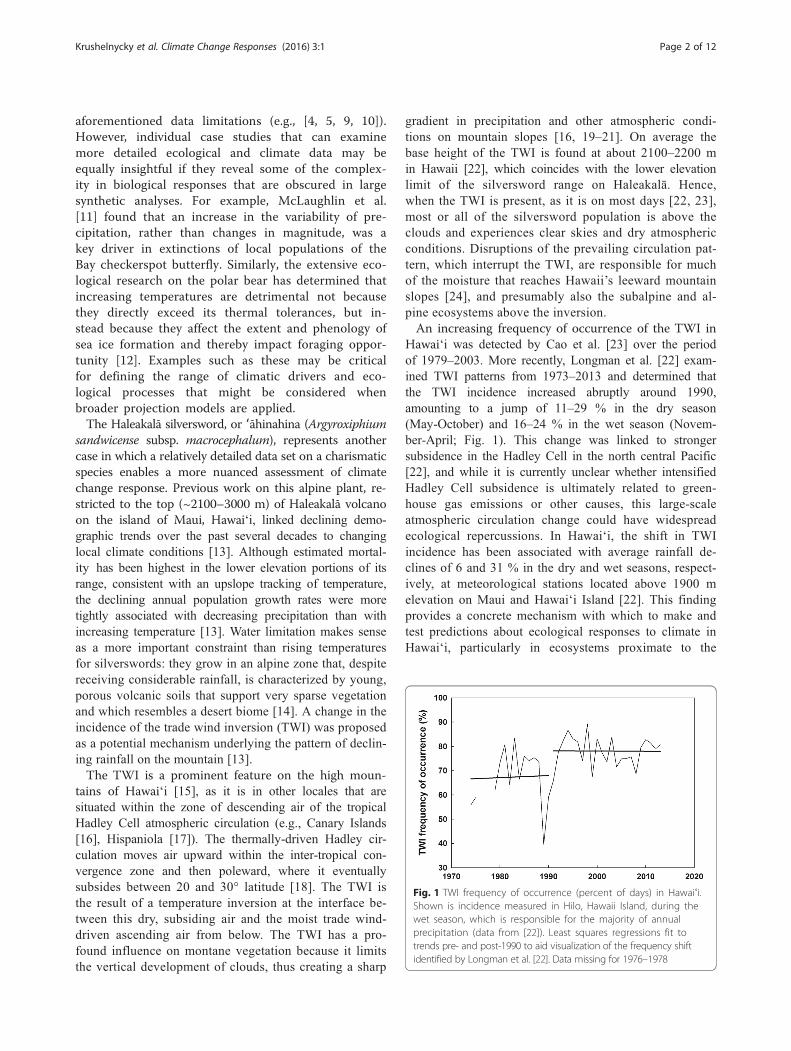
Fig. 1 TWI frequency of occurrence (percent of days) in Hawaiʻi.Shown is incidence measured in Hilo, Hawaii Island, during thewet season, which is responsible for the majority of annualprecipitation (data from [22]). Least squares regressions fit totrends pre- and post-1990 to aid visualization of the frequency shiftidentified by Longman et al. [22]. Data missing for 1976–1978

Krushelnycky et al. Climate Change Responses (2016) 3:1 Page 2 of 12

aforementioned data limitations (e.g., [4, 5, 9, 10]).However, individual case studies that can examinemore detailed ecological and climate data may beequally insightful if they reveal some of the complex-ity in biological responses that are obscured in largesynthetic analyses. For example, McLaughlin et al.[11] found that an increase in the variability of pre-cipitation, rather than changes in magnitude, was akey driver in extinctions of local populations of theBay checkerspot butterfly. Similarly, the extensive eco-logical research on the polar bear has determined thatincreasing temperatures are detrimental not becausethey directly exceed its thermal tolerances, but in-stead because they affect the extent and phenology ofsea ice formation and thereby impact foraging oppor-tunity [12]. Examples such as these may be criticalfor defining the range of climatic drivers and eco-logical processes that might be considered whenbroader projection models are applied.The Haleakalā silversword, or ʻāhinahina (Argyroxiphium

sandwicense subsp. macrocephalum), represents anothercase in which a relatively detailed data set on a charismaticspecies enables a more nuanced assessment of climatechange response. Previous work on this alpine plant, re-stricted to the top (~2100–3000 m) of Haleakalā volcanoon the island of Maui, Hawaiʻi, linked declining demo-graphic trends over the past several decades to changinglocal climate conditions [13]. Although estimated mortal-ity has been highest in the lower elevation portions of itsrange, consistent with an upslope tracking of temperature,the declining annual population growth rates were moretightly associated with decreasing precipitation than withincreasing temperature [13]. Water limitation makes senseas a more important constraint than rising temperaturesfor silverswords: they grow in an alpine zone that, despitereceiving considerable rainfall, is characterized by young,porous volcanic soils that support very sparse vegetationand which resembles a desert biome [14]. A change in theincidence of the trade wind inversion (TWI) was proposedas a potential mechanism underlying the pattern of declin-ing rainfall on the mountain [13].The TWI is a prominent feature on the high moun-

tains of Hawaiʻi [15], as it is in other locales that aresituated within the zone of descending air of the tropicalHadley Cell atmospheric circulation (e.g., Canary Islands[16], Hispaniola [17]). The thermally-driven Hadley cir-culation moves air upward within the inter-tropical con-vergence zone and then poleward, where it eventuallysubsides between 20 and 30° latitude [18]. The TWI isthe result of a temperature inversion at the interface be-tween this dry, subsiding air and the moist trade wind-driven ascending air from below. The TWI has a pro-found influence on montane vegetation because it limitsthe vertical development of clouds, thus creating a sharp

gradient in precipitation and other atmospheric condi-tions on mountain slopes [16, 19–21]. On average thebase height of the TWI is found at about 2100–2200 min Hawaii [22], which coincides with the lower elevationlimit of the silversword range on Haleakalā. Hence,when the TWI is present, as it is on most days [22, 23],most or all of the silversword population is above theclouds and experiences clear skies and dry atmosphericconditions. Disruptions of the prevailing circulation pat-tern, which interrupt the TWI, are responsible for muchof the moisture that reaches Hawaii’s leeward mountainslopes [24], and presumably also the subalpine and al-pine ecosystems above the inversion.An increasing frequency of occurrence of the TWI in

Hawaiʻi was detected by Cao et al. [23] over the periodof 1979–2003. More recently, Longman et al. [22] exam-ined TWI patterns from 1973–2013 and determined thatthe TWI incidence increased abruptly around 1990,amounting to a jump of 11–29 % in the dry season(May-October) and 16–24 % in the wet season (Novem-ber-April; Fig. 1). This change was linked to strongersubsidence in the Hadley Cell in the north central Pacific[22], and while it is currently unclear whether intensifiedHadley Cell subsidence is ultimately related to green-house gas emissions or other causes, this large-scaleatmospheric circulation change could have widespreadecological repercussions. In Hawaiʻi, the shift in TWIincidence has been associated with average rainfall de-clines of 6 and 31 % in the dry and wet seasons, respect-ively, at meteorological stations located above 1900 melevation on Maui and Hawaiʻi Island [22]. This findingprovides a concrete mechanism with which to make andtest predictions about ecological responses to climate inHawaiʻi, particularly in ecosystems proximate to the

Krushelnycky et al. Climate Change Responses (2016) 3:1 Page 3 of 12

TWI (e.g., [25, 26], and may have relevance to other loca-tions strongly influenced by the TWI.Previously reported population trends in the Haleakalā

silversword were derived from a group of demographyplots, combined with range-wide patterns in recent mor-tality that were inferred from a single population survey[13]. In the present study, we build on these resultsusing a time series of population-wide censuses con-ducted roughly every decade since 1971, in addition to apair of earlier projections from regional counts, whichtogether span the past 80 years of demographic historyfor this species. We first use this data set to create aclearer picture of population recovery from ananthropogenically-caused low point in the early 20th

century, which is thought to have represented adrastic reduction relative to the 19th century [27].This history provides a backdrop against which wethen examine the role of changing climate, includinga shift in the incidence of the TWI, in influencingspatiotemporal patterns in more recent silverswordpopulation trajectories.

ResultsDecadal census resultsThe total census counts for the five censuses, as well astotal counts adjusted for differences in spatial coverageamong censuses, are presented in Table 1. Of 111 countsectors demarcating the silversword population, onlyone appears to have lost all plants since the censuseswere initiated. The aggregation of plants in this sectorlocated on the range periphery was last verified to be ex-tant in the 1991 census, when it numbered 106 individ-uals; no live plants could be found in 2001 or 2013. Thecoefficients of variation (CV), measured across censuses,for counts corresponding to each of 19 larger regionscommon to all five censuses had a wide range, from 0.16to 1.12, indicating that the degree of temporal variationdiffered strongly among regions. The CV for counts onKa Moa o Pele cinder cone from 1971–2013 was rela-tively low (0.34) and similar to that for the adjustedpopulation totals for the same period (0.29). Counts forthis cone and the adjusted population totals were also

Table 1 Total population estimates from each of the fivedecadal censuses. Actual census totals and totals adjusted fordifferences in spatial coverage among censuses are shown

Census year Total census count Adjusted total census count

1971 43,325 49,750

1982 47,640 54,096

1991 64,724 73,951

2001 49,498 54,455

2013 30,709 30,709

fairly strongly correlated with one another for the fivecensuses (Pearson r = 0.812, p = 0.095, n = 5). Plants onthis cone therefore appear to fluctuate in a similar fash-ion to that of the entire population, and two early countson this cone may be relatively good indicators of totalpopulation size at those times. Based on the number ofplants counted on Ka Moa o Pele in 1935, combinedwith the range in the proportion of plants on this conerelative to the total population count in the fivecomplete censuses (1971–2013), the population size in1935 is projected to have been between 11,587 and18,329. The population size in 1962, using the samemethod, is projected to have been between 17,719 and28,029. Our estimate for 1935 is several times higherthan the prior estimate of 4000 plants calculated by pro-jecting the number of flowering plants on Ka Moa o Pelecone as a proportion of the total number of floweringplants in 1935 [28].The estimated population trend over time, including

the two early projections, is depicted in Fig. 2. Thepopulation appeared to rebound strongly until 1991, butthe two most recent censuses in 2001 and 2013 recordedstrong population declines (Fig. 2a). Temporal trendsover the five census periods, separated by elevation zone,are shown in Fig. 2b,c. The lower portion of the silver-sword range encompasses the vast majority of plants,and thus showed a trend very similar to the overallpopulation, including strong declines since 1991 (Fig. 2b).In contrast, the upper portion, which supports relativelyfew plants, has continued to increase over the entire rec-ord. Trends depicted on a relativized scale suggest thatrates of population growth in the two elevation zoneswere very similar up to 1991, but diverged sometimearound this date, and that the continued growth in thehigher elevation areas has slowed since 2001 (Fig. 2c).

Count error rates and estimated true population sizeFor 18 count sectors, the ratio of the original countto a second more accurate ‘true’ count ranged from0.32 to 0.96. This indicates that all original observa-tions undercounted the actual number of plants inthe sector by varying degrees. This count error rate,which has smaller values with greater error, wasnegatively related to the log(observation distance)(r2 = 0.544, p < 0.001), and positively related to thelog(original count) (r2 = 0.417, p = 0.004). The latterrelationship was unexpected, but likely simply indi-cates that this proportional error rate is more sensi-tive to smaller numbers/aggregations of plants.However, these smaller aggregations contribute lessto the population total, making the higher errorrates less important. A multiple regression model in-cluding both log(observation distance) and log(origi-nal count) explained the most variation in the count

Fig. 2 Estimated Haleakalā silversword population trend over time. Adjusted census totals for the entire population from 1971 to 2013 shown in(a), along with population size estimates for 1935 and 1962, with lower and upper bounds projected from counts on a single cinder cone (seeMethods). Population trends for lower and upper elevation zones, calculated from 19 regions surveyed in all five censuses, plotted by (b) numberof plants, and (c) number of plants relativized by highest totals in each zone

Krushelnycky et al. Climate Change Responses (2016) 3:1 Page 4 of 12

error rate (r2 = 0.619, p = 0.001, Table 2), even thoughlog(original count) was only marginally significantwhen accounting for log(observation distance). Weused the fitted regression with both explanatory vari-ables to predict the count error rates, true counts,and the 95 % prediction intervals for all 111 countsectors in the 2013 census. This resulted in an esti-mated true total population size in 2013 of 39,355

Table 2 Multiple regression model for the count error rate in18 count sectors censused in 2013. Total model r2 = 0.619,p = 0.001

Term Coefficient SE t p

intercept 0.622 0.358 1.74 0.103

log(observation distance) −0.219 0.078 −2.82 0.013

log(original count) 0.217 0.126 1.72 0.106

plants (95 % prediction interval: 26,257–84,806). Be-cause the reported prediction interval was actually asummation of the 111 individual prediction intervals,the large range includes scenarios in which most orall of the counts were subject to the widest range oferrors around their individual predictions. We there-fore regard the large outer bounds of the interval tobe extremely conservative and highly unlikely.

Influence of climate on decadal trendsDecadal-scale population change was significantly andpositively correlated with average rainfall totals forthe dry (May-Oct) and wet (Nov-Apr) seasons andfor the water year (Nov-Oct) during the inter-censusperiods (linear regression r2 = 0.815, p = 0.036 for dry;r2 = 0.880, p = 0.018 for wet; r2 = 0.919, p = 0.010 forannual; n = 5 for each). For wet season and annual

Krushelnycky et al. Climate Change Responses (2016) 3:1 Page 5 of 12

rainfall averages, these relationships were best fit withquadratic equations, and the strongest relationshipexisted between percent population change per dec-ade and the average annual rainfall over the wateryear during the inter-census period (Fig. 3a; r2 =0.991, p = 0.009). Relationships between decadal-scalepopulation change and average air temperatures dur-ing the inter-census periods were negative but notstatistically significant (linear regression r2 = 0.546, p= 0.154 for dry season; r2 = 0.475, p = 0.198 for wetseason; r2 = 0.548, p = 0.153 for annual; n = 5 foreach). Quadratic equations did not improve the fit fortemperature. The negative relationship betweendecadal-scale population change and average TWI fre-quency during the inter-census periods was statisti-cally significant for the dry season (linear regressionr2 = 0.918, p = 0.042; n = 4; Fig. 3b) but not for thewet season (r2 = 0.663, p = 0.186; n = 4).

Fig. 3 Relationships between decadal-scale population change and climateseveral climate measures, including (a) average annual rainfall during the inTWI frequency of occurrence during the inter-census periods (r2 = 0.918, p =

On an annual scale, estimated rainfall in silverswordhabitat was significantly and negatively related toTWI frequency of occurrence from 1973 to 2013 inboth the dry (r2 = 0.289, p = 0.001; n = 38) and wet (r2

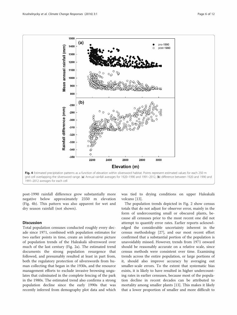
= 0.371, p < 0.001; n = 37) seasons, although there wasconsiderable variance around these relationships. Fordecadal averages, wet season rainfall was significantlyand negatively associated with wet season incidenceof the TWI (r2 = 0.946, p = 0.027; n = 4), but dry sea-son rainfall was not significantly related to dry seasonTWI incidence (r2 = 0.359, p = 0.401; n = 4). Plots ofaverage annual rainfall in silversword habitat acrosselevation show that precipitation was considerablylower after 1990 than before 1990, and that precipita-tion generally decreased with increasing elevation dur-ing both periods (Fig. 4a). However, differencesbetween the periods displayed a distinct nonlinear,threshold-type relationship with elevation, wherein the

. Silversword population change was significantly associated withter-census periods (r2 = 0.991, p = 0.009), and (b) average dry season0.042)

Fig. 4 Estimated precipitation patterns as a function of elevation within silversword habitat. Points represent estimated values for each 250 mgrid cell overlapping the silversword range. (a) Annual rainfall averages for 1920–1990 and 1991–2012, (b) difference between 1920 and 1990 and1991–2012 averages for each cell

Krushelnycky et al. Climate Change Responses (2016) 3:1 Page 6 of 12

post-1990 rainfall difference grew substantially morenegative below approximately 2350 m elevation(Fig. 4b). This pattern was also apparent for wet anddry season rainfall (not shown).

DiscussionTotal population censuses conducted roughly every dec-ade since 1971, combined with population estimates fortwo earlier points in time, create an informative pictureof population trends of the Haleakalā silversword overmuch of the last century (Fig. 2a). The estimated trenddocuments the strong population resurgence thatfollowed, and presumably resulted at least in part from,both the regulatory protection of silverswords from hu-man collecting that began in the 1930s, and the resourcemanagement efforts to exclude invasive browsing ungu-lates that culminated in the complete fencing of the parkin the 1980s. The estimated trend also confirms a strongpopulation decline since the early 1990s that wasrecently inferred from demography plot data and which

was tied to drying conditions on upper Haleakalāvolcano [13].The population trends depicted in Fig. 2 show census

totals that do not adjust for observer error, mainly in theform of undercounting small or obscured plants, be-cause all censuses prior to the most recent one did notattempt to quantify error rates. Earlier reports acknowl-edged the considerable uncertainty inherent in thecensus methodology [27], and our most recent effortconfirmed that a substantial portion of the population isunavoidably missed. However, trends from 1971 onwardshould be reasonably accurate on a relative scale, sincecensus methods were consistent over time. Examiningtrends across the entire population, or large portions ofit, should also improve accuracy by averaging outsmaller-scale errors. To the extent that systematic biasexists, it is likely to have resulted in higher undercount-ing rates in earlier censuses, because most of the popula-tion decline in recent decades can be attributed tomortality among smaller plants [13]. This makes it likelythat a lower proportion of smaller and more difficult to

Krushelnycky et al. Climate Change Responses (2016) 3:1 Page 7 of 12

observe plants existed at the times of the most recentcensuses. In this respect, the 58.5 % estimated decline inpopulation size from 1991 to 2013 may be viewed asconservative. Using an independent method and datasource, Krushelnycky et al. [13] arrived at a similar esti-mate of the magnitude of population declines over thepast two decades in the lower portion of the silverswordrange, which encompasses the vast majority of thepopulation.Average annual rainfall was very strongly correlated

with decadal-scale changes for the population as a whole(Fig. 3a). This also supports the findings of Krushelnyckyet al. [13], which documented a negative relationshipbetween annual population growth rates in demographyplots and annual and seasonal measures of rainfall. Thecongruence between these results measured at two dif-ferent spatial and temporal scales strengthens the inter-pretation that declines in the Haleakalā silverswordpopulation since the early 1990s have been caused bychanges in climate patterns. There are no obvious alter-nate explanations for the increase in plant mortality anddecline in seedling recruitment during this period [13],such as plant diseases, invasive pests, or loss of pollina-tors [29]. Unlike rainfall, air temperature was not foundto be significantly correlated with population changes ei-ther on the decadal scale evaluated here, or on the an-nual scale assessed by Krushelnycky et al. [13]. However,statistical power to detect such relationships was low inthe present study, and temperature is often linked toother climate variables on a regional scale, includingrainfall. This can make it difficult to separate their ef-fects, especially when sample sizes are small. In real-ity, it is likely that a suite of climate variables wereaffected by the increased frequency of the TWIaround 1990 [22, 30].The synchrony between the upward shift in TWI inci-

dence and the abrupt reversal in the silversword popula-tion trajectory is striking, and makes this climatic shift acompelling mechanism that may be responsible, at leastin part, for strengthening water deficits in the alpinehabitat and for causing deteriorating silversword demo-graphic trends. TWI incidence was negatively correlatedwith rainfall totals in silversword habitat on both annualand decadal time scales, most consistently during thewet season. Coefficients of determination were relativelylow (but highly statistically significant) on the annualscale, suggesting that additional factors are important indetermining the magnitude of rainfall from year to year.For instance, TWI incidence may be strongly tied to thefrequency of precipitation events above its base height,but may be more loosely linked to precipitation totals.Beyond precipitation, TWI presence affects other climatevariables that also influence plant water status. Forexample, on upper Haleakalā, trends since 1990

indicate conditions that have undoubtedly promotedgreater water stress for silverswords and other plants,including decreases in rainfall, relative humidity andcloud attenuation of sunlight, and associated increasesin solar radiation, vapor pressure deficit and potentialevapotranspiration [30, 31]. Ultimately, TWI incidenceduring the dry season was a significant predictor ofdecadal-scale silversword population changes (Fig. 3b),while wet season TWI incidence was not. However,as previously noted, a longer time series could resultin stronger statistical relationships between wet seasonand/or annual TWI incidence and silversword populationgrowth rates.Differences in population trends across elevation also

point to a heterogeneous spatial response to the chan-ging conditions described above. Although we detectedconsiderable variation among census regions in the de-gree to which they fluctuated over time, a coherent di-vergence in trajectories was apparent when grouping thelower and upper portions of the population (Fig. 2b,c).The decadal censuses, therefore, confirmed a gradient inmortality across elevation that was previously and inde-pendently inferred from spatial patterns of live and deadplants [13]. The divergence among lower and upper por-tions of the population occurred around 1990, whenlower elevation areas began their decline while upperelevation areas continued to grow rapidly until around2000, at which point this rate of growth slowed. Relevantto this pattern, spatial rainfall estimates indicate thatwhile there was greater rainfall at low elevations than athigh elevations both before and after 1990 (Fig. 4a), themagnitude of change in rainfall across this temporalinflection point was distinctly non-linear with respectto elevation. Specifically, areas below approximately2350 m experienced notably larger precipitation de-clines than areas above this elevational threshold(Fig. 4b). The zone below the threshold correspondsto the area that is typically directly above the TWIbase height, suggesting that an increase in TWI inci-dence impacts precipitation directly above it moststrongly, by more frequently restricting upward flowof moist air that would otherwise ascend higher onthe mountain. It is unknown whether this magnitudeof intensified precipitation decline is ecologically mean-ingful for silverswords, but it may underestimate the ac-tual degree of moisture reduction for plants in this zone.A lower frequency of clouds rising above the average TWIbase height would also reduce the opportunity for foginterception, which is thought to be an important sourceof water for silverswords [32].Differences in silversword mortality across elevation

may therefore be tied to spatial differences in precipita-tion change, rather than to spatial differences in absoluteprecipitation. Such a pattern could arise in several ways.

Krushelnycky et al. Climate Change Responses (2016) 3:1 Page 8 of 12

One possibility is that variation in drought tolerance ex-ists across the population. Specifically, plants located athigher elevations, which are almost always situatedabove the TWI, may have acquired a greater tolerance towater stress by virtue of local adaptation or a phenotypicresponse to development in more arid conditions. Incomparison, plants in lower elevation/higher precipitationzones have experienced greater mortality from rainfall re-ductions despite receiving more rainfall, contemporan-eously, than higher elevation plants. Inherent differencesin drought tolerance across elevation and rainfall gradientshave been suggested in other plants, including tropical al-pine rosette species [33–36]. Alternatively, the magnitudeof deviation from the norm may be more important than,or act synergistically with, any possible differences indrought tolerance. For example, greater dieback in lowelevation populations that experience more intense waterstress during episodes of severe drought has been docu-mented for other plants [37–39]. Identifying the relativeimportance of these mechanisms as causes of differentialsilversword mortality is the subject of current research.The long-term census record shows that, given protec-

tion from collection and grazing and with sufficientrainfall, silverswords are capable of relatively rapid popu-lation growth, as occurred in the 1960s and again in the1980s. If the rate of undercounting we measured in themost recent census is typical or even conservative, it islikely that the population reached or exceeded 95,000plants by the late 1980s. Even the current estimate of ap-proximately 40,000 plants represents a considerable im-provement over the estimated number of plants aroundthe 1930s, which proved to be an adequate remnant forsuccessful recovery later in the century. However, thestrong links between population growth rates andclimate conditions mean that future persistence or re-covery will be dependent on a wetter climate regime,particularly as temperatures rise and potentially lead tohigher rates of evapotranspiration. Unfortunately, recentdownscaled climate projections for Hawaiʻi predict ahigher frequency and lower base height for the TWI[40], as well as decreased precipitation in both the wetand dry seasons for upper Haleakalā under future warm-ing scenarios [7].

ConclusionsThis case study provides several illustrations of how theincorporation of greater climatic and organismal detailcan better characterize the range of possible ecologicalresponses to climate change [41]. First, while the gen-eral pattern of intensified mortality at the lower end ofthe silversword range matches simple predictions of up-slope tracking of rising temperatures, closer examin-ation indicates that silverswords are likely respondingto a combination of changes in precipitation, insolation,

and evaporative demand (which is influenced bytemperature). These changes appear to be mediated lo-cally by a shift in the TWI prevalence, and perhapsmore broadly by alterations to larger atmosphericcirculation patterns, rather than by steadily rising airtemperatures.Second, predictions of climate change impacts on

montane biota have commonly focused on changes inthe base height of the TWI [21, 26, 42–45], as well as onchanges in the lifting condensation level, which corre-sponds to the cloud base height [46, 47], because of theobvious repercussions on montane cloud forests.Changes in the base height of the TWI in Hawaiʻi arenot yet apparent [22], but our results strongly suggestthat changes in TWI incidence alone can have severeecological impacts.Finally, although very little climate-related range re-

duction has occurred for silverswords thus far, the pat-tern of mortality indicates that the wetter, rather thandrier, portions of the current range will likely be the firstto see retractions in response to drying conditions. Thiscounterintuitive outcome may be a consequence of aninteraction between regional differences in drought tol-erance, the distribution of such differences relative toprecipitation and temperature gradients on the moun-tain, and the way in which atmospheric circulationchanges have altered these gradients. Unexpected spatialresponses such as this have been predicted in situationswhere species have locally-adapted populations, becausethe narrower climate envelopes of constituent popula-tions render projections based on species-wide toler-ances inaccurate [48, 49]. Continued monitoring andphysiological research on the Haleakalā silversword mayprovide documentation of this type of complex distribu-tional effect of climate change.

MethodsStudy site and speciesThe Haleakalā silversword, Argyroxyphium sandwicensesubsp. macrocephalum (A. Gray) Meyrat, is a federally-listed threatened taxon in the family Asteraceae thatoccurs only on East Maui, Hawaiʻi. The Mauna Keasilversword (Argyroxyphium sandwicense subsp. sand-wicense (A. Gray) Meyrat), is sister to the Haleakalāsilversword, and is a federally-listed endangered subspe-cies growing at high elevations on Mauna Kea volcano,Hawaiʻi Island. Two additional silversword taxa grow onWest Maui and Mauna Loa, Hawaiʻi Island. Unspecifiedreferences to silversword plants in this study refer to theHaleakalā subspecies.The Haleakalā silversword is a long-lived (estimated

20–90 year, [50]), monocarpic, acaulescent rosette plantthat today grows on the largely barren cinder cones,cinder flats, and rocky cliffs in a broad geographic

Krushelnycky et al. Climate Change Responses (2016) 3:1 Page 9 of 12

area spanning the central to western portions ofHaleakalā crater up to the summit, in the alpine zonefrom 2150 to 3050 m elevation (roughly 2300 ha).Long-term averages of annual rainfall across thesilversword range are estimated to vary from 1018 to1352 mm [51], with approximately 70 % of this fallingin the wet season (November-April, [13]. Silversword dis-tributions within the total range on upper Haleakalāvolcano are clumped, with distinct aggregations often sep-arated by large areas devoid of individuals. These aggrega-tions were first comprehensively mapped and censused byH. Kobayashi in 1971 [32]. Following Kobayashi’s recom-mendations, a total population census was subsequentlyrepeated approximately every decade (see below).Early accounts suggest that the silversword population

underwent a dramatic decline around the turn of the19th century, owing to ungulate browsing and humanvandalism [27]. Anecdotal descriptions by several visitorsto Haleakalā crater in the 1800s imply a large abundanceof plants, including the description of “thousands of sil-verswords … making the hillside look like winter ormoonlight” in 1873 [52]. By the 1920s, however, seriousconcern arose among National Park staff and local resi-dents, as it was apparent that the population had beendecimated by feral goats and cattle and by zealous over-collection by people [27]. As before, no numbers wereattached to these observations, with the exception of anestimate of “barely 100 plants” for the entire populationmade by a botanist in 1927 [53]. This was almost cer-tainly a drastic underestimate, as a careful count ofplants on one cinder cone, Ka Moa o Pele, in 1935 re-corded 1470 plants [27]. This 1935 count, and a re-peated count of the same cone in 1962, are the onlyreliable figures for silversword abundances prior to 1971.The 1935 count was previously used to estimate a totalpopulation of approximately 4000 in that year [28], byprojecting the proportion of flowering plants on Ka Moao Pele (88 of 1470) onto the entire population (in which217 flowering plants were counted). In response to theaforementioned concern regarding silversword persist-ence, rigorous protections against plant collection wereinstituted by the National Park Service in the 1930s, andferal ungulates were controlled through hunting andwere eventually completely excluded in the 1980s with afence encircling the park [27].

Census proceduresTotal population censuses were conducted in 1971,1982, 1991, 2001 and 2013. In all censuses prior to 2013,one to three observers attempted to count all plants dur-ing a two to four week period. For this purpose, thesilversword range was divided into 82 sectors that corre-sponded to a combination of known silversword aggre-gations and topographical features such as cinder cones

or portions of cinder cones, and observers visited asmany of these sectors as possible during each census.Total number of plants in each sector was estimated bycounting all visible live plants with either the nakedeye or with binoculars, depending on the observer’sdistance. Observation distances are known to havevaried tremendously, from several meters or tens ofmeters in flat regions that can be traversed on foot,to several hundreds of meters in regions situated onsteep cinder cone faces or on distant cliffs. However, theseobservation distances and/or vantage points were not re-corded. Methods of earlier censuses are also reported inKobayashi [32] and Loope & Crivellone [27].In the 2013 census, the procedure was modified to

allow comparison with prior censuses while improvingmethods for future censuses. Four observers completedthe census between October 2013 and March 2014,using the same methods described above. However, thecount sectors were modified to more accurately repre-sent current boundaries of silversword aggregations, ra-ther than relying more heavily on topographic features,and the resulting 111 sectors were mapped in GIS(Geographic Information Systems) to allow more ac-curate relocation and delineation in future censuses(Additional file 1: Figure S1). In addition, observationdistances were estimated for each region, either byestimating average distances to plants in regions thatwere walked through, or by using ArcGIS™ 10.2.2(ESRI, Redlands, CA, USA) to measure the distancesfrom observer vantage points to the midpoints of sec-tors in cases where binoculars were used. Finally,more effort was expended in the 2013 census, com-pared to prior censuses, to visit all previously re-ported locations supporting silverswords, making itthe most thorough census to date.

Census comparisons over timeBecause each census counted plants in a slightly differ-ent subset of sectors, and because these sectors weremodified somewhat in 2013, we delineated 19 regionsthat were fully counted in all five censuses, groupingmultiple sectors within each region, to enable compari-son between censuses (Additional file 1: Figure S1).Sectors were generally grouped by cinder cone orcontiguous lava flows. These 19 regions comprisedfrom 86.7 to 99.6 % of the actual total counts in eachcensus, with the lowest percentage (86.7 %) corre-sponding to 2013, the most spatially complete census.Therefore, the summed totals of the 19 regions incommon for each census were subsequently dividedby 0.867 to calculate an adjusted total count for eachcensus, which accounted for areas missed and madethe censuses directly comparable. This procedure as-sumes that the small minority of areas not counted in

Krushelnycky et al. Climate Change Responses (2016) 3:1 Page 10 of 12

the 1971 to 2001 censuses fluctuated in the samemanner as the remainder of the population.Counts of plants on Ka Moa o Pele cinder cone were

1470 in 1935 and 2248 in 1962 [32]. This coneaccounted for between 8.0 and 12.7 % of the fiveadjusted census totals (1971–2013). We therefore usedthis range to calculate a rough estimate of the lower andupper bounds for the total population in 1935 and 1962,by dividing the Ka Moa o Pele counts in those years by0.127 and 0.080. We feel that this is likely to be a moreaccurate method for estimating the total population sizethan the one used previously, in which the proportion ofplants flowering on the cone was projected to the entirepopulation [28]. This is because proportions of plantsflowering are known to vary considerably from region toregion in a given year, much more so than the magni-tude of variation observed in the proportion of plants onKa Moa o Pele cone relative to the estimated populationtotal over the five censuses.Related work has suggested that silverword population

declines over the past two decades have been mostsevere in lower elevation portions of the range [13]. Toassess whether the decadal censuses have recorded asimilar pattern, the 19 common geographic regions de-scribed above, which spanned an elevation of approxi-mately 2200 m to 2700 m, were split into two evenelevation zones (2200–2450 m, 2450–2700 m), and tem-poral trends between 1971 and 2013 were compared ineach zone. We took this approach of lumping plantnumbers across large geographic areas, rather than relat-ing percent population change within each region to itselevation, because strong temporal variation and/orcounting error in smaller geographic units led to veryhigh and probably unrealistic variation in the resultantpercent population changes, making spatial patterns dif-ficult to detect.

Assessment of count error rate and true total populationestimateFor 18 of the 111 count sectors in the 2013 census, weperformed a second ‘true’ count, in which every liveplant was individually approached and coordinates wererecorded using a Garmin eTrex Legend H GPS unit(Garmin Ltd., Olathe, KS, USA). The ratios of the initialcounts to the second true counts were used as estimatesof count error rates for these sectors. Error rates werethen regressed against the log-transformed observationdistance and the log-transformed initial count (numberof plants). These relationships were subsequently usedto estimate count error rates (and 95 % prediction inter-vals) and to predict the true plant numbers for all 111sectors in the 2013 census, based on the observation dis-tances and number of plants estimated for each of thesesectors. To avoid negative as well as unreasonably high

predictions, we bounded the lower ends of the 95 % pre-diction intervals for the count error rates to 0.1, whichseems reasonable given that the lowest measured counterror rate was 0.32 (see Results). The resultant predictedtrue counts and 95 % intervals were summed to estimatethe true total population size in 2013.

Influence of climate on decadal trendsWe examined the explanatory power of patterns in rain-fall, air temperature and the frequency of occurrence ofthe TWI on the magnitude and direction of decadal-scale population changes. For rainfall, we used a data-base of spatially-explicit (250 m grid cell resolution)hind-casted monthly rainfall estimates for the island ofMaui from 1920 through 2012 [54]. We extracted allgrid cells coinciding with the silversword distribution,and used these to calculate the average dry season(May-October), wet season (November-April) and annual(by water year, November-October) rainfall across thesilversword range during each inter-census period. Rainfalldata for 2012–2013 were taken from the average of sixweather stations installed across the silversword range in2010. Monthly mean air temperature data through 2010were taken from the Haleakalā Ranger Station locatedat the park headquarters, 2125 m elevation (NationalClimatic Data Center). Air temperature data from2010 to 2013 were taken from HaleNet station 151,also located at the Haleakalā NP headquarters [55].We used the combined data to calculate average dryseason, wet season, and annual air temperatures foreach inter-census period. Frequency of occurrence ofthe TWI was calculated from atmospheric soundingdata collected daily at 2 pm HST in Hilo, HawaiʻiIsland, from 1973 to 2013; these data are maintainedby the University of Wyoming and can be accessed athttp://weather.uwyo.edu/upperair/sounding/html. TWIpresence was determined according to the methods inLongman et al. [22], and frequency of daily occur-rence (%) was calculated for all dry seasons, wet sea-sons and water years possessing at least 75 % of dailyreadings. This resulted in TWI data gaps during the1971–1982 inter-census period: for the dry seasonand wet season, respectively, 64 and 54 % of seasonshad available data, while only 45 % of water yearshad available data during this period. We thereforechose to not use the water year data, and only calcu-lated average dry season and wet season TWI fre-quency of occurrence for each inter-census period.There were no gaps in the TWI data after the 1970s.We used the above inter-census climate averages as

explanatory variables in simple linear regressions withpercent decadal change in population size as the re-sponse variable. For the latter, we used the adjusted cen-sus totals, and standardized the percent population

Krushelnycky et al. Climate Change Responses (2016) 3:1 Page 11 of 12

change between each census to ten year periods. Becausethere are only four inter-census periods, we added a fifthperiod, 1962–1971, to increase sample size, by using theaverage of the lower and upper bounds of the 1962total population estimate (however, only rainfall andtemperature data were available for this earlierperiod). Because non-linearity was suggested in someof the fitted relationships, we also attempted quad-ratic regressions against the rainfall and temperaturedata, but not against the TWI data which only hadfour data points. Due to the small sample sizes andintercorrelations, we did not fit multiple regressionsusing combinations of explanatory climate variables.To test the influence of the TWI on rainfall pat-

terns in Haleakalā silversword habitat, we regressedseasonal rainfall totals against TWI frequency of oc-currence for all years with available data between1973 and 2013 (n = 38 and 37 for dry and wet sea-sons, respectively); we also regressed the decadal aver-ages of dry and wet season rainfall on decadalaverages of TWI incidence (n = 4 for each). We fur-ther examined graphically how the reported shift inTWI frequency around 1990 may have differentiallyaffected rainfall across elevation within silverswordhabitat. To do this, we plotted the mean estimated annualrainfall for the periods 1920–1990 and 1991–2012, foreach 250 m grid cell within silversword habitat (n = 377),as a function of elevation. We also plotted the differencebetween these two time periods (pre- and post-1990) rela-tive to elevation.

Additional file

Additional file 1: Figure S1. Map of the top of Haleakala volcano,showing census counting areas. Red polygons indicate 111 count sectors,black polygons indicate the 19 larger regions that were surveyed in allfive censuses. (PDF 371 kb)

Competing interestsThe authors declare that they have no competing interests.

Authors’ contributionsStudy design was conceived by PDK, FS, KS and LLL. Data were collected byFS, KS, LLL, RJL, AGF, TWG and PDK, and analyzed by PDK, RJL and AGF.Manuscript was drafted by PDK, RJL, AGF and TWG. All authors read andapproved the final manuscript.

AcknowledgementsWe would like to acknowledge and thank Herbert Kobayashi for laying thefoundation for Haleakalā silversword population mapping, monitoring, andecological research, and for inspiring the continuation of this work. JesseFelts provided assistance in the most recent census. We are grateful toHaleakalā National Park for financial and logistical support. Funding was alsoprovided by the Pacific Islands Climate Change Cooperative, the PacificIslands Climate Science Center, and the Hauʻoli Mau Loa Foundation.Haleakalā NP and US Fish and Wildlife Service provided research permits.

Author details1Department of Plant and Environmental Protection Sciences, University ofHawaiʻi at Mānoa, Honolulu, HI 96822, USA. 2Pacific Cooperative Studies Unit,

University of Hawaiʻi at Mānoa, Honolulu, HI 96822, USA. 3Department ofGeography, University of Hawaiʻi at Mānoa, Honolulu, HI 96822, USA. 4PacificIsland Ecosystems Research Center, US Geological Survey, Honolulu, HI96813, USA. 5Present address: 751 Pelenaka Pl., Makawao, HI 96768, USA.

Received: 1 September 2015 Accepted: 8 January 2016

References1. Parmesan C. Ecological and evolutionary responses to recent climate

change. Annu Rev Ecol Syst. 2006;37:637–69.2. Crimmins SM, Dobrowski SZ, Greenberg JA, Abatzoglou JT, Mynsberge AR.

Changes in climatic water balance drive downhill shifts in plant species’optimum elevations. Science. 2011;331:324–7.

3. Tingley MW, Koo MS, Moritz C, Rush AC, Beissenger SR. The push and pullof climate change causes heterogeneous shifts in avian elevational ranges.Glob Change Biol. 2012;18:3279–90.

4. VanDerWal J, Murphy HT, Kutt AS, Perkins GC, Bateman BL, Perry JJ, et al.Focus on poleward shifts in species’ distribution underestimates thefingerprint of climate change. Nat Clim Chang. 2012;3:239–43.

5. Gillings S, Balmer DE, Fuller RJ. Directionality of recent bird distribution shiftsand climate change in Great Britain. Glob Chang Biol. 2015;21:2155–68.

6. IPCC. Summary for policymakers. In: Stocker TF et al., editors. Climatechange 2013: The physical science basis. Contribution of working group I tothe Fifth Assessment Report of the Intergovernmental Panel on ClimateChange. Cambridge: Cambridge University Press; 2013.

7. Elison Timm O, Giambelluca TW, Diaz HF. Statistical downscaling of rainfallchanges in Hawaiʻi based on the CMIP5 global model projections.J Geophys Res-Atmos. 2015;120:92–112.

8. Dobrowski SZ, Abatzoglou J, Swanson AK, Greenberg JA, Mynsberge AR,Holden ZA, et al. The climate velocity of the contiguous United Statesduring the 20th century. Glob Chang Biol. 2013;19:241–51.

9. Parmesan C, Yohe G. A globally coherent fingerprint of climate changeimpacts across natural systems. Nature. 2003;421:37–42.

10. Root TL, Price JT, Hall KR, Schneider SH, Rosenzweig C, Pounds JA.Fingerprints of global warming on wild animals and plants. Nature.2003;421:57–60.

11. McLaughlin JF, Hellmann JJ, Boggs CL, Ehrlich PR. Climate changehastens population extinctions. Proc Natl Acad Sci U S A.2002;99:6070–4.

12. Stirling I, Derocher AE. Effects of climate warming on polar bears: a reviewof the evidence. Glob Chang Biol. 2012;18:2694–706.

13. Krushelnycky PD, Loope LL, Giambelluca TW, Starr F, Starr K, Drake DR, et al.Climate-associated population declines reverse recovery and threaten futureof an iconic high-elevation plant. Glob Chang Biol. 2013;19:911–22.

14. Leuschner C, Schulte M. Microclimatological investigations in the tropicalalpine scrub of Maui, Hawaiʻi: evidence for a drought-induced alpinetimberline. Pac Sci. 1991;45:152–68.

15. Giambelluca TW, Nullet D. Influence of the trade-wind inversion on theclimate of a leeward mountain slope in Hawai‘i. Clim Res. 1991;1:207–16.

16. Fernández-Palacios JM, de Nicolás JP. Altitudinal pattern of vegetationvariation on Tenerife. J Veg Sci. 1995;6:183–90.

17. Martin PH, Fahey TJ. Mesoclimatic patterns shape the striking vegetationmosaic in the Cordillera Central, Dominican Republic. Arct Antarct Alp Res.2014;46:755–65.

18. Diaz HF, Bradley RS. The Hadley circulation: present, past and future.Dordrecht: Kluwer; 2004.

19. Kitayama K, Mueller-Dombois D. Vegetation of the wet windward slope ofHaleakala, Maui, Hawaii. Pac Sci. 1992;46:197–220.

20. Crausbay SD, Hotchkiss SC. Strong relationships between vegetation andtwo perpendicular climate gradients high on a tropical mountain in Hawaiʻi.J Biogeogr. 2010;37:1160–74.

21. Martin PH, Fahey TJ, Sherman RE. Vegetation zonation in a neotropicalmontane forest: environment, disturbance and ecotones. Biotropica.2010;43:533–43.

22. Longman RJ, Diaz HF, Giambelluca TW. Sustained increases in lowertropospheric subsidence over the central tropical North Pacific drives adecline in high elevation rainfall in Hawaiʻi. J Clim. 2015;28:8743–59.

23. Cao G, Giambelluca TW, Stevens DE, Schroeder TA. Inversion variability inthe Hawaiian trade wind regime. J Clim. 2007;20:1145–60.

Krushelnycky et al. Climate Change Responses (2016) 3:1 Page 12 of 12

24. Giambelluca TW, Schroeder TA. The physical environment: climate. In: JuvikSP, Juvik JO, editors. Atlas of Hawaiʻi. 3rd ed. Honolulu: University of HawaiʻiPress; 1998. p. 49–59.

25. Banko PC, Camp RJ, Farmer C, Brinck KW, Leonard DL, Stephens RM.Response of palila and other subalpine Hawaiian forest bird species toprolonged drought and habitat degradation by feral ungulates. BiolConserv. 2013;157:70–7.

26. Crausbay SD, Frazier AG, Giambelluca TW, Longman RJ, Hotchkiss SC.Moisture status during a strong El Nino explains a tropical montane cloudforest’s upper limit. Oecologia. 2014;175:273–84.

27. Loope LL, Crivellone CF. Status of the Haleakalā silversword: past andpresent. Technical report CNPRSU-58. Honolulu: University of Hawaiʻi; 1986.

28. USFWS. Recovery plan for the Maui plant cluster. Portland: US Fish andWildlife Service; 1997.

29. Krushelnycky PD. Evaluating the interacting influences of pollination, seedpredation, invasive species and isolation on reproductive success in athreatened alpine plant. PLoS ONE. 2014;9(2):e88948. doi:10.1371/journal.pone.0088948.

30. Longman RJ, Giambelluca TW, Nullet MA, Loope LL. Climatology ofHaleakalā. Technical report CNPRSU-193. Honolulu: University of Hawaiʻi;2015.

31. Longman RJ, Giambelluca TW, Alliss RJ, Barnes ML. Temporal solar radiationchange at high elevations in Hawaiʻi. J Geophys Res-Atmos. 2014;119.doi:10.1002/2013JD021322.

32. Kobayashi HK. Ecology of the silversword, Argyroxiphium sandwicense DC.(Compositae), Haleakalā Crater, Hawaiʻi. PhD Thesis. Honolulu: University ofHawaiʻi; 1973.

33. Baruch Z. Elevational differentiation in Espeletia schultzii (Compositae), agiant rosette plant of the Venezuelan Paramos. Ecology. 1979;60:85–98.

34. Meinzer FC, Goldstein GH, Rundel PW. Morphological changes along analtitude gradient and their consequences for an Andean giant rosette plant.Oecologia. 1985;65:278–83.

35. Zhang H, DeWald LE, Kolb TE, Koepke DF. Genetic variation inecophysiological and survival responses to drought in two native grasses:Koeleria macrantha and Elymus elymoides. West N Am Naturalist.2011;71:25–32.

36. Vasques A, Chrino E, Vilagrosa A, Vallejo VR, Keizer JJ. The role of seedprovenance in the early development of Arbutus unedo seedlings undercontrasting watering conditions. Environ Exp Bot. 2013;96:11–9.

37. Allen CD, Breshears DD. Drought-induced shift of a forest-woodlandecotone: rapid landscape response to climate variation. Proc Natl Acad SciU S A. 1998;95:14839–42.

38. McDowell NG, Allen CD, Marshall L. Growth, carbon-isotope discrimination,and drought-associated mortality across a Pinus ponderosa elevationaltransect. Glob Chang Biol. 2010;16:399–415.

39. Worrall JJ, Egeland L, Eager T, Mask RA, Johnson EW, Kemp PA, et al. Rapidmortality of Populus tremuloides in southwestern Colorado. USA Forest EcolManag. 2008;255:686–96.

40. Lauer A, Zhang C, Elison-Timm O, Wang Y, Hamilton K. Downscaling ofclimate change in the Hawaiʻi Region using CMIP5 results: on the choice ofthe forcing fields. J Clim. 2013;26:10006–30.

41. Helmuth B, Russell BD, Connell SD, Dong Y, Harley CDG, Lima FP, et al.Beyond long-term averages: making biological sense of a rapidly changingworld. Clim Chang Responses. 2014;1:6.

42. Loope LL, Giambelluca TW. Vulnerability of island tropical montane cloudforests to climate change, with special reference to East Maui, Hawaiʻi. ClimChang. 1998;39:503–17.

43. Sperling FN, Washington R, Whittaker RJ. Future climate change of thesubtropical North Atlantic: implications for the cloud forests of Tenerife.Clim Chang. 2004;65:103–23.

44. Lloret F, González-Mancebo JM. Altitudinal distribution patterns ofbryophytes in the Canary Islands and vulnerability to climate change. Flora.2011;206:769–81.

45. Harter DEV, Irl SDH, Seo B, Steinbauer MJ, Gillespie R, Triantis KA, et al.Impacts of global climate change on the floras of oceanic islands –Projections, implications and current knowledge. Perspect Plant Ecol.2015;17:160–83.

46. Pounds JA, Fogden MPL, Campbell JH. Biological response to climatechange on a tropical mountain. Nature. 1999;398:611–5.

47. Foster P. The potential negative impacts of global climate change ontropical montane cloud forests. Earth-Sci Rev. 2001;55:73–106.

48. O’Neill GA, Hamann A, Wang T. Accounting for population variationimproves estimates of the impact of climate change on species’ growthand distribution. J Appl Ecol. 2008;45:1040–9.

49. Kuo ESL, Sanford E. Geographic variation in the upper thermal limits of anintertidal snail: implications for climate envelope models. Mar Ecol-Prog Ser.2009;388:137–46.

50. Rundel PW, Witter MS. Population dynamics and flowering in a Hawaiianalpine rosette plant, Argyroxiphium sandwicense. In: Rundel PW, Smith AP,Meinzer FC, editors. Tropical alpine environments: plant form and function.New York: Cambridge Univ. Press; 1994. p. 295–306.

51. Giambelluca TW, Chen Q, Frazier AG, Price JP, Chen Y-L, Chu P-S, et al.Online Rainfall Atlas of Hawaiʻi. B Am Meteorol Soc. 2013;94:313–6.doi:10.1175/BAMS-D-11-00228.1.

52. Bird IL. Six months in the Sandwich Islands. London: John Murray; 1890.53. Degener O. Plants of Hawaiʻi National Parks. Ann Arbor: Braum-Blumfield;

1930.54. Frazier AG, Giambelluca TW, Diaz HF, Needham HL. Comparison of

geostatistical methods to spatially interpolate month-year rainfall for theHawaiian Islands. Int J Climatol. 2015. doi:10.1002/joc.4437.

55. HaleNet. HaleNet Haleakalā climate network. 2015. http://climate.socialsciences.hawaii.edu/HaleNet/HaleNet.htm. Accessed 15 March 2015.

• We accept pre-submission inquiries

• Our selector tool helps you to find the most relevant journal

• We provide round the clock customer support

• Convenient online submission

• Thorough peer review

• Inclusion in PubMed and all major indexing services

• Maximum visibility for your research

Submit your manuscript atwww.biomedcentral.com/submit

Submit your next manuscript to BioMed Central and we will help you at every step: