Department of Economics and Business Aarhus University Fuglesangs Allé 4 DK-8210 Aarhus V Denmark Email: [email protected]Tel: +45 8716 5515 Changes in persistence, spurious regressions and the Fisher hypothesis Robinson Kruse, Daniel Ventosa-Santaulària and Antonio E. Noriega CREATES Research Paper 2013-11
Changes in persistence, spurious regressions and the Fisher
hypothesis
Robinson Kruse, Daniel Ventosa-Santaulària
and Antonio E. Noriega
CREATES Research Paper 2013-11
Changes in persistence, spurious regressions
and the Fisher hypothesis ∗
Robinson Kruse† Daniel Ventosa-Santaularia‡ Antonio E. Noriega§
April 16, 2013
Abstract
Declining inflation persistence has been documented in numerous studies. When such series are ana-lyzed in a regression framework in conjunction with other persistent time series, spurious regressionsare likely to occur. We propose to use the coefficient of determination R2 as a test statistic to distinguishbetween spurious and genuine regressions in situations where time series possibly (but not necessar-ily) exhibit changes in persistence. To this end, we establish some limit theory for the R2 statisticand conduct a Monte Carlo study where we investigate its finite-sample properties. Finally, we applythe test to the Fisher equation for the U.S. and Mexico. Contrary to a rejection using cointegrationtechniques, the R2-based test offers strong evidence favourable to the Fisher hypothesis.
Key Words: Changes in persistence, Spurious regression, Fisher hypothesis.
JEL classification: C12, C22, E31, E43
1 Introduction
Structural breaks in autoregressive models have been studied widely, see Perron (2006) for a comprehen-sive survey on the recent developments in this field. A special kind of a structural break is a change in∗Participants at the 20th Annual Symposium of the Society for Nonlinear Dynamics and Econometrics in Istanbul, Turkey and
at the Statistical Week 2012 in Vienna, Austria provided useful comments. Moreover, the authors thank Matei Demetrescu andMichael Massmann for helpful discussions on an earlier draft of the paper. Part of this research was carried out while the secondauthor was visiting CREATES at Aarhus University, Denmark; their kind hospitality is greatly appreciated. Robinson Krusegratefully acknowledges support from CREATES - Center for Research in Econometric Analysis of Time Series (DNRF78),funded by the Danish National Research Foundation.
†Leibniz University Hannover [School of Economics and Management, Institute of Statistics, Konigsworther Platz 1, D-30167 Hannover, Germany] and CREATES, Aarhus University [Department of Economics and Business, Fuglesangs Alle 4,DK-8210 Aarhus V, Denmark. E-mail: [email protected].]
‡Centro de Investigacion y Docencia Economicas, CIDE [Carretera Mexico-Toluca 3655, Col. Lomas de Sta Fe, Del. AlvaroObregon, Mexico D.F, C.P. 01210. E-mail address: [email protected] ]
§Banco de Mexico [Direccion General de Emision, Legaria 691, Col. irrigacion, Mexico D.F., Mexico. E-mail address:[email protected] ] and Universidad de Guanajuato [Department of Economics and Finance, Cerro El Establo S/N,Guanajuato, Gto. Mexico.]
1
persistence. It is characterized by a change in the order of integration of a time series. For instance, afirst-order autoregressive (AR) model exhibits a change in persistence if the AR parameter equals oneduring the pre-break sample and less than unity (in absolute value) after the breakpoint. Persistence de-clines in the sense that the process switches from being I(1) to I(0). Main contributions to this topic areKim (2000), Leybourne, Kim, Smith, and Newbold (2003), Busetti and Taylor (2004), Kurozumi (2005),Harvey, Leybourne, and Taylor (2006), Leybourne, Kim, and Taylor (2007) and Leybourne, Taylor, andKim (2007) inter alia. As Perron (2006) points out, changing persistence has been an important featureof economic time series. In particular, inflation rates are typically found to display declines in persis-tence, see e.g. O’Reilly and Whelan (2005), Kumar and Okimoto (2007), Halunga, Osborn, and Sensier(2008), Noriega and Ramos-Francia (2009), Kang, Kim, and Morley (2009), Kejriwal (2012) and Koure-tas and Wohar (2012). It is a natural approach to investigate the consequences of changing persistencein a regression framework, which has not been conducted yet (at least to our best knowledge). Importantregressions involving inflation series are the Fisher equation, Taylor rules and the Phillips curve amongstothers. Asymptotic theory is well known and established for the case of stable persistence, but there is alack of it when it comes to structural changes in the persistence of time series.
This paper studies the asymptotic properties of standard regression techniques under changes in per-sistence. It turns out that the problem of spurious regressions becomes important. Spurious regressionshave been considered, since its reappraisal in Granger and Newbold (1974), as a pervasive problem intime series econometrics. It occurs when “[. . . ] a pair of independent series, but with strong temporalproperties, is found apparently related according to standard inference [. . . ].1” The theoretical frameworkprovided by Phillips (1986) explained the phenomenon using non-standard asymptotics. Spurious regres-sion may indeed occur under a wide array of data generating processes, whether these are stationary ornot: driftless unit roots (Phillips 1986), higher-order integrated processes (Marmol 1995, Marmol 1996)],unit root with drifts (Entorf 1997), stationary processes (Granger, Hyung, and Jeon 2001), long-memoryprocesses, stationary or not (Marmol 1998, Tsay and Chung 2000), trend stationary processes, with andwithout breaks and combinations thereof.2
Our large-sample results show that the estimation of regression models can lead to spurious inferencewhen at least one of the variables possesses a change in persistence. Indeed, the t-ratios associated to theestimates diverge, whether the variables are truly linearly related or not; such a result is quite intuitive.Nevertheless, our results also provide a clear suggestion for testing whether the relationship is spuriousor meaningful. This paper proposes the coefficient of determination R2 as a test statistic. It is shown thatthe R2 exhibits a non-standard limit distribution depending on the unknown breakpoints when no relationbetween the variables exists. Under the alternative hypothesis of a meaningful linear relationship, the R2
converges to unity. Critical values of the R2 statistic are obtained via simulations. Empirical size andpower properties of the test are investigated in a Monte Carlo study. It appears that the test performs wellunder a relatively vast array of alternative DGPs and situations.
1Granger, Hyung, and Jeon (2001).2See Noriega and Ventosa-Santaularia (2007). A brief survey of the literature concerning spurious regression can be found in
Ventosa-Santaularia (2009).
2
As an empirical application, we study the Fisher equation for Mexico and the United States. Whilestandard econometric tools like cointegration analysis do not lead to supportive results, the situation isdifferent when applying the R2 test: We find strong evidence for the empirical validity of the Fisher effect.Our approach is related to many previous studies in this field. Most of them consider unit root tests,cointegration techniques and structural breaks. Our study complements the literature by considering theconsequences of changing inflation persistence for testing the Fisher effect as a novelty. Importantly, wepropose a simple OLS regression-based test for the Fisher hypothesis which is a long standing issue inmonetary economics. In direct connection, the persistence properties of inflation and nominal (and real)interest rates are analyzed.
An important early contribution is Barsky (1987), who studies the effect of changing inflation per-sistence in relation to the Fisher hypothesis and forecastability of inflation.3 Koustas and Serletis (1999)apply unit root and stationarity tests to inflation and interest rates and test for cointegration amongst thesevariables in order to test for the Fisherian link. Rapach and Weber (2004) re-examine and extend a studyby Rose (1988) by using advanced unit root and cointegration techniques. Lanne (2006) suggests a non-linear bivariate mixture autoregressive model for interest rates and inflation. A nonlinear cointegrationapproach is taken by Christopoulos and Leon-Ledesma (2007). Panel cointegration methods for testingthe Fisher hypothesis are proposed in Westerlund (2008). Recently, Tsong and Lee (2013) apply quantilecointegration methods. Jensen (2009) investigates the consequences of fractionally integrated processesfor tests of the Fisher hypothesis. Structural breaks in deterministic terms (i.e. intercept and trend) inrelation to the Fisher effect are studied in Malliaropulos (2000), Rapach and Wohar (2005), Lai (2008)and Haug, Beyer, and Dewald (2011). A Markov switching analysis of the US real interest rate has beenput forward by Garcia and Perron (1996). These studies underline the importance of integration ordersand structural breaks for testing the Fisher hypothesis.
The remaining body of the paper is organized as follows. Section 2 presents the setup and the asymp-totic results together with simulated critical values. In Section 3, the Monte Carlo simulation study isdescribed and results are presented. Empirical applications are given in Section 4. Finally, conclusionsare drawn in Section 5. Mathematical proofs are provided in the Appendix.
2 Setup and asymptotic results
This article reconsiders the problem of spurious regressions in a bivariate setup were variables (y,x) areallowed to exhibit a single structural break in their order of integration. The focus lies on the bivariate setupto illustrate the problem and the suggested testing procedure. Clearly, the methodology can be extended tomultiple regressors without further complications. We study the asymptotic behaviour of OLS estimationand inference under a variety of possible situations. If changes in persistence are neglected, spuriousregressions are likely to occur. By I(1/0), we denote a variable that exhibits a decline in persistence atsome breakpoint λ. The case of increasing persistence, i.e. I(0/1), is treated analogously. We analyze
3A detailed survey is provided by Neely and Rapach (2008).
3
Case DGP for y DGP for x Remarks
y,x are independentM1 I(1) I(1) Both series are constant I(1) processesM2 I(1/0) I(1) y exhibits a decline in persistence, x is a constant I(1) processM3 I(1) I(1/0) y is a constant I(1) process, x exhibits a decline in persistenceM4 I(1/0) I(1/0) Both series exhibit a decline in persistence at the same breakpointM4’ I(1/0) I(1/0) Both series exhibit a decline in persistence at different breakpointsM5 I(d) I(d) Both series are fractionally integrated (of the same order)M5’ I(dy) I(dx) Both series are fractionally integrated (of different orders)
y,x are dependentM6 I(1) I(1) Both series are cointegrated, no change in persistence occursM7 I(1/0) I(1/0) Both series are first cointegrated, then related (after the breakpoint)
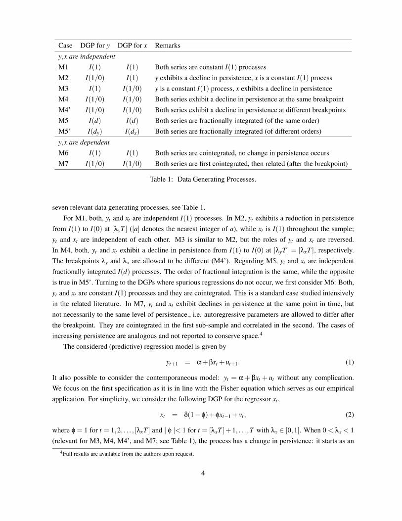
Table 1: Data Generating Processes.
seven relevant data generating processes, see Table 1.For M1, both, yt and xt are independent I(1) processes. In M2, yt exhibits a reduction in persistence
from I(1) to I(0) at [λyT ] ([a] denotes the nearest integer of a), while xt is I(1) throughout the sample;yt and xt are independent of each other. M3 is similar to M2, but the roles of yt and xt are reversed.In M4, both, yt and xt exhibit a decline in persistence from I(1) to I(0) at [λyT ] = [λxT ], respectively.The breakpoints λy and λx are allowed to be different (M4’). Regarding M5, yt and xt are independentfractionally integrated I(d) processes. The order of fractional integration is the same, while the oppositeis true in M5’. Turning to the DGPs where spurious regressions do not occur, we first consider M6: Both,yt and xt are constant I(1) processes and they are cointegrated. This is a standard case studied intensivelyin the related literature. In M7, yt and xt exhibit declines in persistence at the same point in time, butnot necessarily to the same level of persistence., i.e. autoregressive parameters are allowed to differ afterthe breakpoint. They are cointegrated in the first sub-sample and correlated in the second. The cases ofincreasing persistence are analogous and not reported to conserve space.4
The considered (predictive) regression model is given by
yt+1 = α+βxt +ut+1. (1)
It also possible to consider the contemporaneous model: yt = α+ βxt + ut without any complication.We focus on the first specification as it is in line with the Fisher equation which serves as our empiricalapplication. For simplicity, we consider the following DGP for the regressor xt ,
xt = δ(1−φ)+φxt−1 + vt , (2)
where φ = 1 for t = 1,2, . . . , [λxT ] and | φ |< 1 for t = [λxT ]+1, . . . ,T with λx ∈ [0,1]. When 0 < λx < 1(relevant for M3, M4, M4’, and M7; see Table 1), the process has a change in persistence: it starts as an
4Full results are available from the authors upon request.
4
I(1) process at the beginning of the sample and becomes I(0) after the breakpoint. When λx = 1 (relevantfor M1, M2, and M6), there is no change in persistence and the process behaves as a random walk alongthe whole sample. As for the DGP of yt , we envisage two informative alternatives:
1. The process is independent of xt and in particular,
yt+1 = µ(1−ρ)+ρyt + et+1 (3)
where ρ = 1 for t = 1,2, . . . , [λyT ] and | ρ |< 1 for t = [λyT ]+1, . . . ,T ; λy ∈ [0,1]. The persistenceproperties are analogous to the ones discussed for the regressor xt above.
2. The variables are allowed to be linearly related to each other. In this case, the DGP of yt correspondsto equation (1). Note that, if xt has a change in persistence in [λxT ], the variables are cointegratedduring the period t = 1 to t = [λxT ]. Afterwards, althhough there is not anymore a long-run equi-librium relationship, xt and yt remain correlated (Model M7).
Some remarks on notation are in order. In the following Theorem 1, convergence in distribution isdenoted as D→, and Wz is a standard Wiener process, i.e., Wz(r) is normally distributed for every r in [0,1];that is Wz(r) ∼ N (0,r). To simplify notation, all integrals are understood to be taken with respect tothe Lebesgue measure, i.e., integrals such as
∫ 10 Wz,
∫ 10 W 2
z ,∫
λ
0 Wz, and∫
λ
0 WxWy are short for∫ 1
0 Wz(r)dr,∫ 10 W 2
z (r)dr,∫
λ
0 Wz(r)dr, and∫
λ
0 WxWy(r)dr, respectively.5 As with the properties of et and vt , we assumethey satisfy Hamilton’s (1994, p. 505) standard assumption, that is:
Assumption 1 Let zt = Ψ(L)εzt = ∑∞j=0 Ψz, jεz,t− j for z = e,v, where ∑
∞j=0 j |Ψz, j |< ∞ and {εz,t} is and
i.i.d sequence with mean zero, variance σ2z , and finite fourth moment.
The derivations in this work hold under more general data generating processes (in particular linearprocesses with stationary martingale difference innovations), but these assumptions are sufficient to giveinsight into the behaviour of the coefficient of determination in the case of a possibly spurious regressionunder changes in persistence.
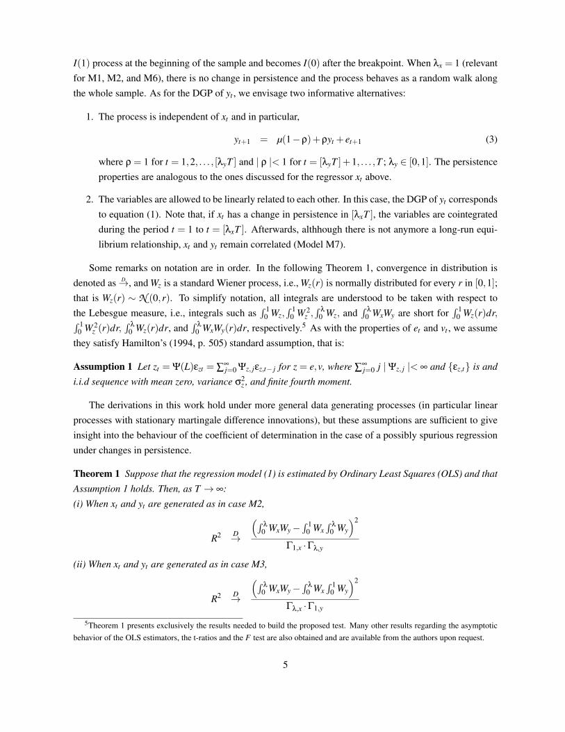
Theorem 1 Suppose that the regression model (1) is estimated by Ordinary Least Squares (OLS) and thatAssumption 1 holds. Then, as T → ∞:(i) When xt and yt are generated as in case M2,
R2 D→
(∫λ
0 WxWy−∫ 1
0 Wx∫
λ
0 Wy
)2
Γ1,x ·Γλ,y
(ii) When xt and yt are generated as in case M3,
R2 D→
(∫λ
0 WxWy−∫
λ
0 Wx∫ 1
0 Wy
)2
Γλ,x ·Γ1,y
5Theorem 1 presents exclusively the results needed to build the proposed test. Many other results regarding the asymptoticbehavior of the OLS estimators, the t-ratios and the F test are also obtained and are available from the authors upon request.
5
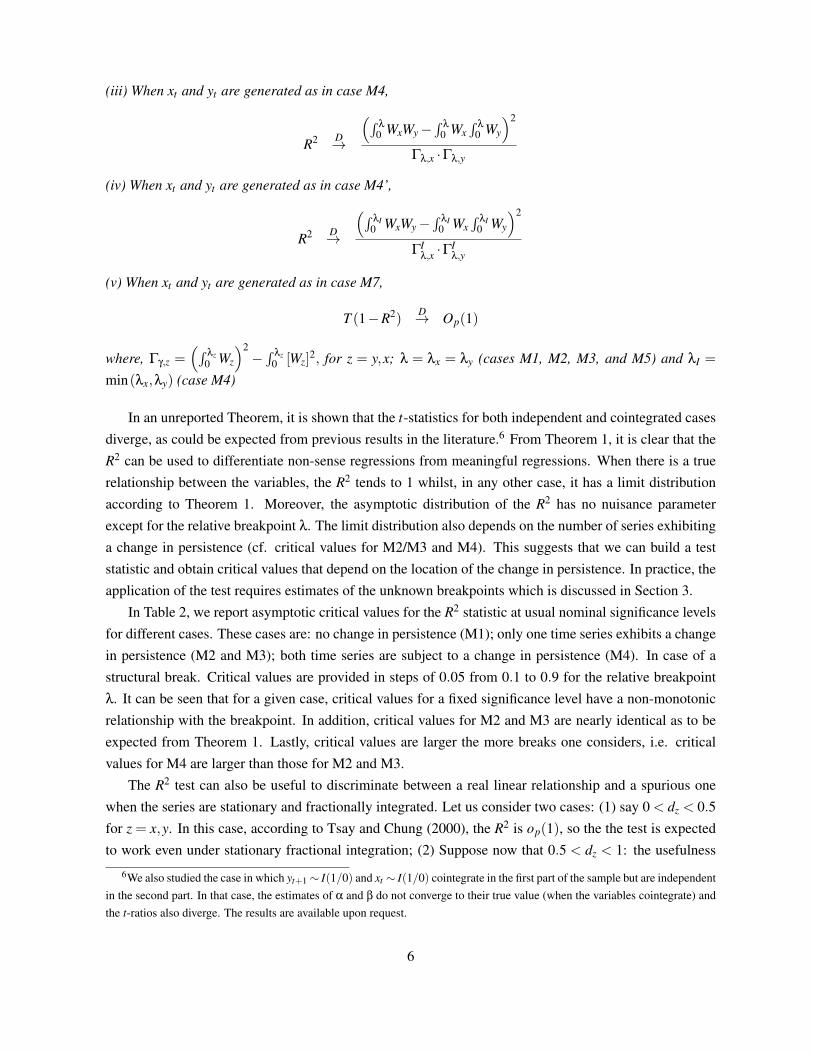
(iii) When xt and yt are generated as in case M4,
R2 D→
(∫λ
0 WxWy−∫
λ
0 Wx∫
λ
0 Wy
)2
Γλ,x ·Γλ,y
(iv) When xt and yt are generated as in case M4’,
R2 D→
(∫λI0 WxWy−
∫λI0 Wx
∫λI0 Wy
)2
ΓIλ,x ·Γ
Iλ,y
(v) When xt and yt are generated as in case M7,
T (1−R2)D→ Op(1)
where, Γγ,z =(∫ λz
0 Wz
)2−
∫ λz0 [Wz]
2, for z = y,x; λ = λx = λy (cases M1, M2, M3, and M5) and λI =
min(λx,λy) (case M4)
In an unreported Theorem, it is shown that the t-statistics for both independent and cointegrated casesdiverge, as could be expected from previous results in the literature.6 From Theorem 1, it is clear that theR2 can be used to differentiate non-sense regressions from meaningful regressions. When there is a truerelationship between the variables, the R2 tends to 1 whilst, in any other case, it has a limit distributionaccording to Theorem 1. Moreover, the asymptotic distribution of the R2 has no nuisance parameterexcept for the relative breakpoint λ. The limit distribution also depends on the number of series exhibitinga change in persistence (cf. critical values for M2/M3 and M4). This suggests that we can build a teststatistic and obtain critical values that depend on the location of the change in persistence. In practice, theapplication of the test requires estimates of the unknown breakpoints which is discussed in Section 3.
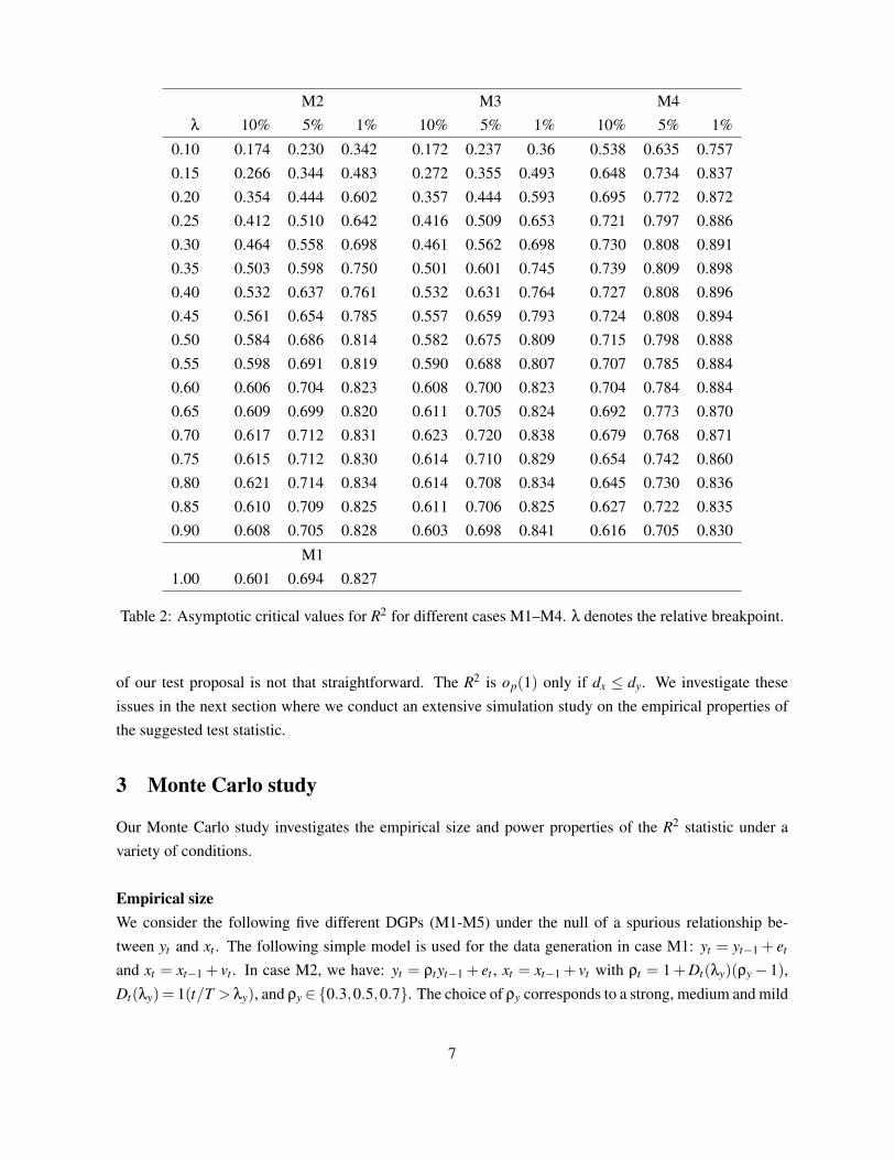
In Table 2, we report asymptotic critical values for the R2 statistic at usual nominal significance levelsfor different cases. These cases are: no change in persistence (M1); only one time series exhibits a changein persistence (M2 and M3); both time series are subject to a change in persistence (M4). In case of astructural break. Critical values are provided in steps of 0.05 from 0.1 to 0.9 for the relative breakpointλ. It can be seen that for a given case, critical values for a fixed significance level have a non-monotonicrelationship with the breakpoint. In addition, critical values for M2 and M3 are nearly identical as to beexpected from Theorem 1. Lastly, critical values are larger the more breaks one considers, i.e. criticalvalues for M4 are larger than those for M2 and M3.
The R2 test can also be useful to discriminate between a real linear relationship and a spurious onewhen the series are stationary and fractionally integrated. Let us consider two cases: (1) say 0 < dz < 0.5for z = x,y. In this case, according to Tsay and Chung (2000), the R2 is op(1), so the the test is expectedto work even under stationary fractional integration; (2) Suppose now that 0.5 < dz < 1: the usefulness
6We also studied the case in which yt+1 ∼ I(1/0) and xt ∼ I(1/0) cointegrate in the first part of the sample but are independentin the second part. In that case, the estimates of α and β do not converge to their true value (when the variables cointegrate) andthe t-ratios also diverge. The results are available upon request.
Table 2: Asymptotic critical values for R2 for different cases M1–M4. λ denotes the relative breakpoint.
of our test proposal is not that straightforward. The R2 is op(1) only if dx ≤ dy. We investigate theseissues in the next section where we conduct an extensive simulation study on the empirical properties ofthe suggested test statistic.
3 Monte Carlo study
Our Monte Carlo study investigates the empirical size and power properties of the R2 statistic under avariety of conditions.
Empirical sizeWe consider the following five different DGPs (M1-M5) under the null of a spurious relationship be-tween yt and xt . The following simple model is used for the data generation in case M1: yt = yt−1 + et
and xt = xt−1 + vt . In case M2, we have: yt = ρtyt−1 + et , xt = xt−1 + vt with ρt = 1+Dt(λy)(ρy− 1),Dt(λy)= 1(t/T > λy), and ρy ∈{0.3,0.5,0.7}. The choice of ρy corresponds to a strong, medium and mild
7
reduction in persistence. The case M3 is analogous. In case M4, we have yt = ρtyt−1+et , xt = φtxt−1+vt ,with ρt as before, φt = 1+Dt(λx)(ρx− 1) and Dt(λx) = 1(t/T > λx). Lastly, case (M5) is specified asfollows: (1−L)dyyt = et , (1−L)dxxt = vt , with 0.5< dy,dx < 1. The case of spurious regressions with frac-tionally integrated time series has been investigated, amongst others, by Marmol (1995), Marmol (1998),and Tsay and Chung (2000). The innovations are drawn from a bivariate standard Normal distributionwith a diagonal covariance matrix. The number of replications equals 5,000 for each single experiment.We consider three different sample sizes: T ∈ {100,300,500} which resemble situations where eitherquarterly or monthly recorded macroeconomic or financial data is analyzed. The breakpoints are locatedeither in the beginning, in the middle or at the end of the sample, i.e. λy,λx ∈ {0.3,0.5,0.7}. The locationof the breakpoints are treated as unknown and thus estimated from the data. For this purpose, we comparethe experimental performance of three different breakpoint estimators which have been suggested in therelated literature on changes in persistence, see Kim, Belaire Franch, and Badilli Amador (2002), Busettiand Taylor (2004) and Leybourne, Kim, and Taylor (2007). In particular, these estimators are given by,
λKBA = argmaxτ
[(1− τ)T ]−2S1(τ)
[τT ]−1S0(τ)
λBT = argmaxτ
[(1− τ)T ]−2S1(τ)
[τT ]−2S0(τ)
λLT K = argminτ
[τT ]−2S0(τ),
with the sum-of-squares,
S0(τ) =[τT ]
∑t=1
(zt −
1[τT ]
[τT ]
∑t=1
zt
)2
S1(τ) =[τT ]
∑t=1
(zt −
1T − [τT ]
T
∑t=[τT ]+1
zt
)2
,
defined for a time series zt , see Hassler and Scheithauer (2011). The criterion functions are maximized(or minimized) over the interval τ ∈ [0.2,0.8] which is a common choice in practice. In case (M4), theminimum of λy and λx determine the critical values. Note that this follows from our theoretical resultsderived in Theorem 1 (iv).The following null hypotheses of spurious regressions can be tested:
H(1)0 : no persistence change in y and x
H(2)0 : persistence change in y
H(3)0 : persistence change in x
H(4)0 : persistence change in both, y and x
In practice, several situations may occur: (i) the user has some prior information or knowledge about theexistence of a change in persistence, (ii) the user applies univariate pre-tests in order to investigate the
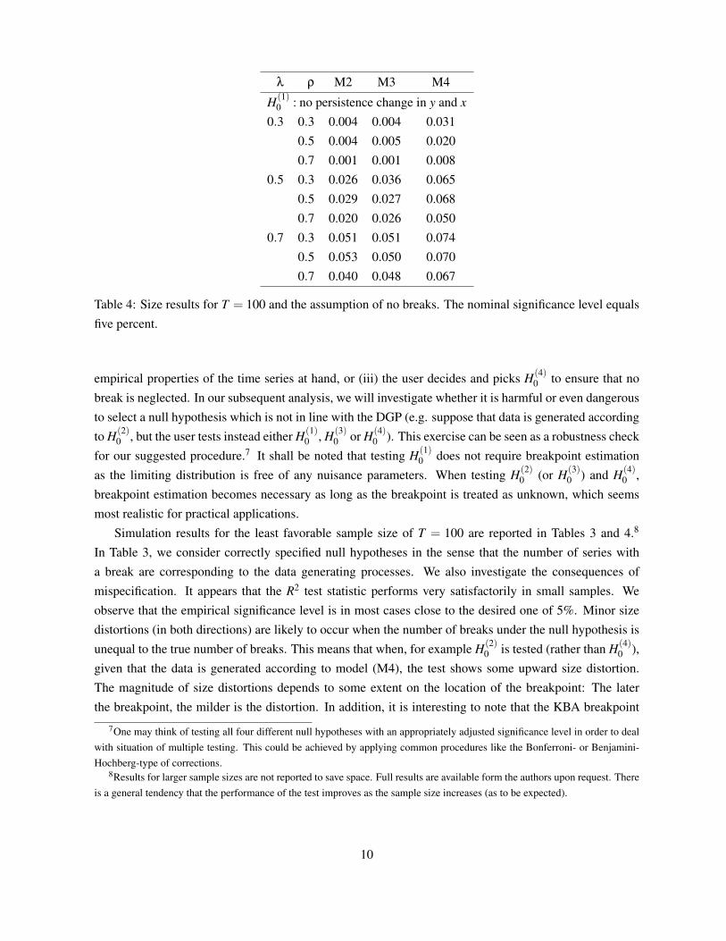
Table 4: Size results for T = 100 and the assumption of no breaks. The nominal significance level equalsfive percent.
empirical properties of the time series at hand, or (iii) the user decides and picks H(4)0 to ensure that no
break is neglected. In our subsequent analysis, we will investigate whether it is harmful or even dangerousto select a null hypothesis which is not in line with the DGP (e.g. suppose that data is generated accordingto H(2)
0 , but the user tests instead either H(1)0 , H(3)
0 or H(4)0 ). This exercise can be seen as a robustness check
for our suggested procedure.7 It shall be noted that testing H(1)0 does not require breakpoint estimation
as the limiting distribution is free of any nuisance parameters. When testing H(2)0 (or H(3)
0 ) and H(4)0 ,
breakpoint estimation becomes necessary as long as the breakpoint is treated as unknown, which seemsmost realistic for practical applications.
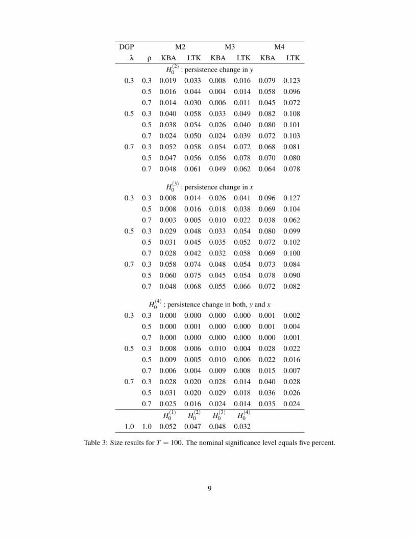
Simulation results for the least favorable sample size of T = 100 are reported in Tables 3 and 4.8
In Table 3, we consider correctly specified null hypotheses in the sense that the number of series witha break are corresponding to the data generating processes. We also investigate the consequences ofmispecification. It appears that the R2 test statistic performs very satisfactorily in small samples. Weobserve that the empirical significance level is in most cases close to the desired one of 5%. Minor sizedistortions (in both directions) are likely to occur when the number of breaks under the null hypothesis isunequal to the true number of breaks. This means that when, for example H(2)
0 is tested (rather than H(4)0 ),
given that the data is generated according to model (M4), the test shows some upward size distortion.The magnitude of size distortions depends to some extent on the location of the breakpoint: The laterthe breakpoint, the milder is the distortion. In addition, it is interesting to note that the KBA breakpoint
7One may think of testing all four different null hypotheses with an appropriately adjusted significance level in order to dealwith situation of multiple testing. This could be achieved by applying common procedures like the Bonferroni- or Benjamini-Hochberg-type of corrections.
8Results for larger sample sizes are not reported to save space. Full results are available form the authors upon request. Thereis a general tendency that the performance of the test improves as the sample size increases (as to be expected).
10
estimators offers the best test performance, closely followed by the LTK breakpoint estimator.9 We alsoconsider the case M1, where no breaks occur, but the null hypothesis covers at least one series with abreak (see the last line of Table 3). In this case, the test performs well. Only when two series with breaksare assumed, the test is slightly conservative.
Results in Table 4 show the empirical size for the case of testing H(1)0 , i.e. no breaks are allowed for.
Data is generated with a break in y and/or in x. This kind of mispecification leads to some distortions:for an early breakpoint (λ = 0.3) the test is conservative, while it is correctly sized or liberal for latebreaks, depending on whether only y or x exhibit a change in persistence or both of them. There is a slighttendency of the test to reject less often as ρ increases.
We now turn to the results for fractionally integrated processes. In general, we find that the R2 testbehaves conservatively as indicated by empirical sizes near zero (unreported to save space). Thereby, weconfirm the claims made in the previous section. In case of a spurious regression amongst fractionallyintegrated series, the test is likely to detect the spurious regression by rarely rejecting in favor of the alter-native. This conclusion is not affected by the particular value of d.
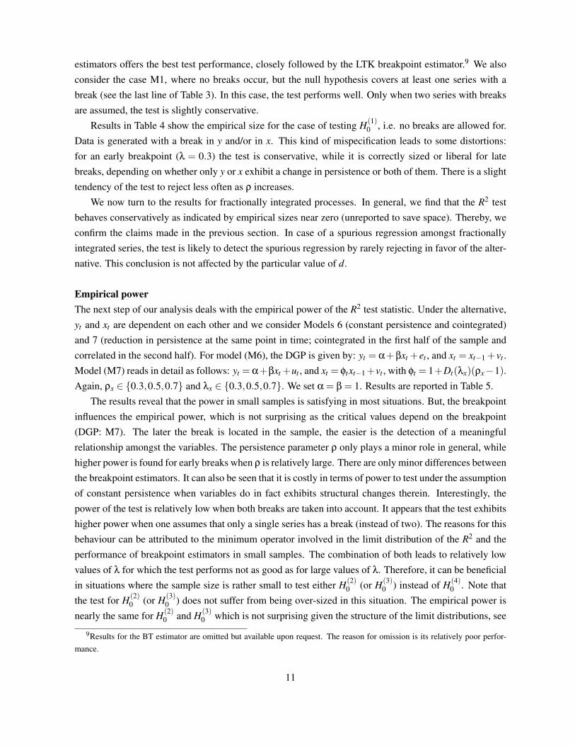
Empirical powerThe next step of our analysis deals with the empirical power of the R2 test statistic. Under the alternative,yt and xt are dependent on each other and we consider Models 6 (constant persistence and cointegrated)and 7 (reduction in persistence at the same point in time; cointegrated in the first half of the sample andcorrelated in the second half). For model (M6), the DGP is given by: yt = α+βxt +et , and xt = xt−1 +vt .Model (M7) reads in detail as follows: yt =α+βxt +ut , and xt = φtxt−1+vt , with φt = 1+Dt(λx)(ρx−1).Again, ρx ∈ {0.3,0.5,0.7} and λx ∈ {0.3,0.5,0.7}. We set α = β = 1. Results are reported in Table 5.
The results reveal that the power in small samples is satisfying in most situations. But, the breakpointinfluences the empirical power, which is not surprising as the critical values depend on the breakpoint(DGP: M7). The later the break is located in the sample, the easier is the detection of a meaningfulrelationship amongst the variables. The persistence parameter ρ only plays a minor role in general, whilehigher power is found for early breaks when ρ is relatively large. There are only minor differences betweenthe breakpoint estimators. It can also be seen that it is costly in terms of power to test under the assumptionof constant persistence when variables do in fact exhibits structural changes therein. Interestingly, thepower of the test is relatively low when both breaks are taken into account. It appears that the test exhibitshigher power when one assumes that only a single series has a break (instead of two). The reasons for thisbehaviour can be attributed to the minimum operator involved in the limit distribution of the R2 and theperformance of breakpoint estimators in small samples. The combination of both leads to relatively lowvalues of λ for which the test performs not as good as for large values of λ. Therefore, it can be beneficialin situations where the sample size is rather small to test either H(2)
0 (or H(3)0 ) instead of H(4)
0 . Note thatthe test for H(2)
0 (or H(3)0 ) does not suffer from being over-sized in this situation. The empirical power is
nearly the same for H(2)0 and H(3)
0 which is not surprising given the structure of the limit distributions, see
9Results for the BT estimator are omitted but available upon request. The reason for omission is its relatively poor perfor-mance.
Table 5: Power results for T = 100. The nominal significance level equals five percent.
Theorem 1. In case of constant persistence (DGP: M6), we find that power is generally higher than forchanging persistence. Similar conclusions can be drawn as for M7.
4 Empirical applications
“The long-run Fisherian theory of interest states that a permanent shock to inflation will cause an equalchange in the nominal interest rate so that the real interest rate is not affected by monetary shocks in thelong run,..., If the nominal interest rate and the inflation rate are each integrated of order one, denotedI(1), then the two variables should cointegrate with a slope coefficient of unity so that the real interestrate is covariance stationary” (Haug, Beyer, and Dewald 2011, p.1). As can be deducted from this para-graph, cointegration seems to be a natural testing strategy to verify empirically the validity of the Fisherhypothesis, or the Fisher effect.
Following the same lines, Phillips (2005) argues that this effect corresponds to the hypothesis thatthe real rate of interest is stationary. Furthermore, when the econometric analysis is carried out usingexpected inflation (as opposed to observed inflation), this effect implies that “the ex ante real rate ofinterest is stationary, so that, under rational expectations and stationary forecast errors for inflation, theFisher effect implies a stationary ex post real rate of interest” Phillips (2005, p.132).
We collect data on interest rates, inflation and inflation expectations for Mexico and the US, to verifythe Fisher hypothesis, not only under the traditional route of cointegration techniques, but also followingthe testing strategy suggested in this paper for the case when variables might be subject to changes inpersistence.
The Mexican data set is built as follows. The inflation series we investigate (πMt ) are monthly, sea-
12
Mexican nominal interest rate (28 days)
1995 2000 2005 2010
02
46
8
Mexican inflation and expected inflation (dashed), estimated breakpoints as vertical lines
1995 2000 2005 2010
02
46
8
US nominal interest rate
1980 1985 1990 1995 2000 2005 2010
05
1015
US inflation and expected inflation (dashed), estimated breakpoints as vertical lines
1980 1985 1990 1995 2000 2005 2010
05
1015
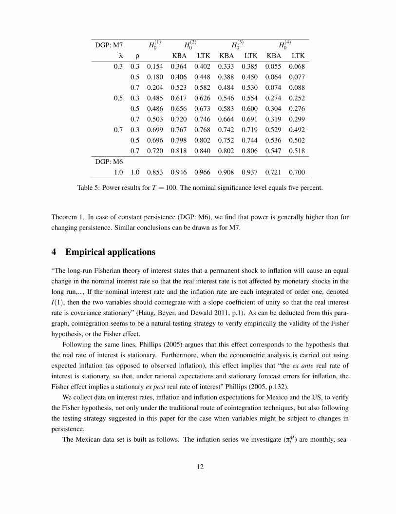
Figure 1: Time series under consideration.
sonally adjusted, based on the national index of consumer prices.10 Inflation expectations (eπMt ) are taken
from the private sector survey of inflation expectations.11 The interest rates used are the GovernmentBonds, CETES at 28 (iM28
t ) and 91 (iM91t ) days.12
For the US, inflation is calculated from the Consumer Price Index of All Urban Consumers (CPI)using the formula 100(CPIt −CPIt−12/CPIt−12).13 Inflation expectations were obtained from the FederalReserve Bank of St. Louis. The definition used is “Median expected price change next 12 months, Surveyof Consumers”.14 The Three Months Treasury Bill was obtained from the Federal Reserve Bank of St.Louis.15
Anticipating the procedures and findings in this section, we first apply unit root test to verify the orderof integration of individual variables. We find that variables follow a unit root process, according to severaltests. Then we test for cointegration using the Johansen procedure. We find that there are either zero or twocointegrating vectors, this last finding contradicting our unit root results. Overall, cointegration techniquesseem not to give empirical support to the Fisherian theory of interest rates for Mexico and the USA.
Given these results, we infer whether there have been any changes in persistence in the individualseries using the approach of Leybourne, Kim, and Taylor (2007) (LKT in what follows), which allows
10Indice Nacional de Precios al Consumidor, INPC, obtained from the Banco de Mexico at http://www.banxico.org.mx.The inflation rate was calculated as πM
t = [(INPCt − INPCt−1)/INPCt−1]100.11See Encuesta de Expectativas del Sector Privado, http://www.banxico.org.mx/estadisticas/index.html12Bond rates were also obtained from Banco de Mexico as average rates in annual percentage points, and then converted to
monthly percentages using the transformation 100 [(1/12) ln(1+annual%CET E/100)] .13Bureau of Labor Statistics, at http://www.bls.gov/cpi/home.htm#data.14Available at http://research.stlouisfed.org/fred2/series/MICH.15Available at http://research.stlouisfed.org/fred2/series/TB3MS.
for multiples changes in persistence, and is robust to changes in the level of the variables. We find thatfor all series but the US interest rate, the M test of LKT detects significant changes in persistence in thedirections I(1)→ I(0), that is, the series become stationary after the break.
Given that cointegration tests are built on the assumption that the series are I(1) throughout, we can-not rely on these tests to verify the Fisher hypothesis (it is not known whether cointegration tests functionproperly under changes in persistence in the underlying variables). Therefore, we apply the procedureproposed in this paper; in particular, we use the R2 in order to verify whether there is a long-run relation-ship between nominal interest rates and the inflation rate, using critical values provided in the paper (theasymptotic critical values for the cases M3 and M4 in Table 2).
Tests for multiple changes in persistenceWe apply the so-called M test, proposed by LKT, which allows to test for multiple changes in the order ofintegration of a time series. As discussed in Noriega and Ramos-Francia (2009), tests for a unit root, asthe augmented Dickey-Fuller (ADF) test, will not be consistent against processes which display changesin persistence, when applied to persistence change series, since the I(1) part will dominate asymptotically.This argument also applies to tests for a single change in persistence, as those of Kim (2000) and Harvey,Leybourne, and Taylor (2006). Additionally, the LKT test allows consistent estimation of the change dates.We start by briefly presenting the basics of the LKT procedure, and after that we report the correspondingempirical results.16 The M test is based on doubly-recursive sequences of DF type unit root statistics:
M ≡ infλ∈(0,1)
infτ∈(λ,1)
DFG(λ,τ), (4)
with corresponding estimators (λ, τ)≡ arg infλ∈(0,1) infτ∈(λ,1) DFG(λ,τ) for τ∈ (λ,1), and λ∈ (0,1), whereDFG(λ,τ) is obtained as the standard t-statistic associated with ρi in the fitted regression that uses thesample observations between [λT ] and [τT ]
′, with α = 1+c/T ,and c =−10. In the empirical applications below, we set λ = 1/T such that λT = 1. As in LKT, we useτ = 0.20.17 For determining the value of ki, we use the BIC for choosing the appropriate lag length forvalues of ki between 0 and 12, for every sample or sub-sample regression computed.
Following Noriega, Capistran, and Ramos-Francia (2012), there are two hypotheses. The null, H0 : theseries is I(1) throughout, and the alternative, H1 : the series undergoes one or more regime shifts betweenI(1) and I(0) behavior. That is, under the alternative, the variable under study (inflation, expected inflation
16The presentation below heavily relies on Noriega, Capistran, and Ramos-Francia (2012), from which further details can beobtained.
17As a robustness check in the empirical applications below, we used different values of τ and obtained qualitatively similarresults.
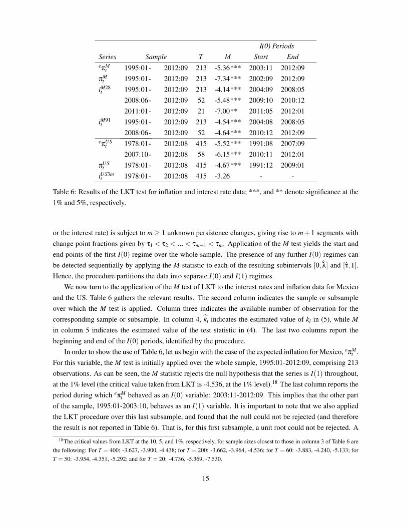
Table 6: Results of the LKT test for inflation and interest rate data; ***, and ** denote significance at the1% and 5%, respectively.
or the interest rate) is subject to m ≥ 1 unknown persistence changes, giving rise to m+1 segments withchange point fractions given by τ1 < τ2 < ... < τm−1 < τm. Application of the M test yields the start andend points of the first I(0) regime over the whole sample. The presence of any further I(0) regimes canbe detected sequentially by applying the M statistic to each of the resulting subintervals [0, λ] and [τ,1].Hence, the procedure partitions the data into separate I(0) and I(1) regimes.
We now turn to the application of the M test of LKT to the interest rates and inflation data for Mexicoand the US. Table 6 gathers the relevant results. The second column indicates the sample or subsampleover which the M test is applied. Column three indicates the available number of observation for thecorresponding sample or subsample. In column 4, ki indicates the estimated value of ki in (5), while Min column 5 indicates the estimated value of the test statistic in (4). The last two columns report thebeginning and end of the I(0) periods, identified by the procedure.
In order to show the use of Table 6, let us begin with the case of the expected inflation for Mexico, eπMt .
For this variable, the M test is initially applied over the whole sample, 1995:01-2012:09, comprising 213observations. As can be seen, the M statistic rejects the null hypothesis that the series is I(1) throughout,at the 1% level (the critical value taken from LKT is -4.536, at the 1% level).18 The last column reports theperiod during which eπM
t behaved as an I(0) variable: 2003:11-2012:09. This implies that the other partof the sample, 1995:01-2003:10, behaves as an I(1) variable. It is important to note that we also appliedthe LKT procedure over this last subsample, and found that the null could not be rejected (and thereforethe result is not reported in Table 6). That is, for this first subsample, a unit root could not be rejected. A
18The critical values from LKT at the 10, 5, and 1%, respectively, for sample sizes closest to those in column 3 of Table 6 arethe following: For T = 400: -3.627, -3.900, -4.438; for T = 200: -3.662, -3.964, -4.536; for T = 60: -3.883, -4.240, -5.133; forT = 50: -3.954, -4.351, -5.292; and for T = 20: -4.736, -5.369, -7.530.
15
very similar interpretation can be made for πMt .
A more complex result is obtained for iM28t , which presents three I(0) periods: 2004:09-2008:05,
2009:10-2010:12, and 2011:05-2012:01. This can be generally interpreted as a series with I(1) behaviourduring the first part (1995:01-2004:08), and a stationary behaviour during the rest of time.19 In fact, allfour series for Mexico can be categorized as having undergone a change in persistence from I(1) into I(0)with the break occurring around the years 2002-2004.20
For the US, both inflation and inflation expectations behaved as I(1) from the beginning of the sample(1978) through 1991, and I(0) onwards -only interrupted towards the end of the sample by the financialcrisis. (the date of the change in persistence does not coincide with the one in Noriega and Ramos-Francia(2009a), who used monthly instead of annual changes in prices). On the other hand, the three monthsTreasury Bill does not exhibit any change in persistence; it behaved as an I(1) variable throughout thesample period (the M test did not detect any significant change in persistence from I(1) to I(0)). Thisresult is consistent with that found by LKT, which applied the M test to monthly data on the log yields on10 year Government bonds for the United States (among other countries), for the period 1978:1-2001:12.They also found the this yield is I(1) throughout their sample.
The general conclusion is that, with the exception of iUS3mt , all variables have undergone a structural
break in their stochastic behaviour, which might explain why we were not able to find cointegration be-tween interest rates and inflation and, therefore, were unable to lend any empirical support to the Fisherhypothesis. From a different perspective, it can be argued that the presence of persistence change in thevariables invalidates the use of cointegration techniques needed to verify the Fisher hypothesis, since coin-tegration necessitates (or assumes) the presence of stochastic trends in the individual variables throughoutthe sample period. To alleviate this problem, we present below an empirical strategy based on our asymp-totic findings, in order to test for the validity of the Fisher hypothesis without resorting to cointegrationtechniques, using instead the R2 statistic, as discussed in section 2 of the paper.
Alternative approach to test the Fisher hypothesisHere we verify whether there can be found a long-run relationship between the nominal interest rate andthe inflation rate for the US and Mexico by applying the approach advocated in this paper, that is, by usingas a test statistic the coefficient of determination, R2. We begin by estimating by OLS equation (4), whichwe reproduce here for convenience:
yt+1 = a+βxt +ut+1, t = 1, ...T
Table 7 below present results from the OLS estimation of this model for each pair of series. In theTable, β is the OLS estimate of the slope parameter, s
βis the estimated standard deviation of β; pβ=0 is
the p−value of the null hypothesis H0 : β = 0 using a t−test statistic, while pβ=1 is the p−value of thenull hypothesis H0 : β = 1. Finally, R2 is the coefficient of determination which will be used to asses thevalidity of the Fisher hypothesis.
19The finding of three aparently separated I(0) periods can be due to changes in the level of the series. See LKT for details.20For the inflation series, the result is consistent with that found in Noriega, Capistran, and Ramos-Francia (2012).
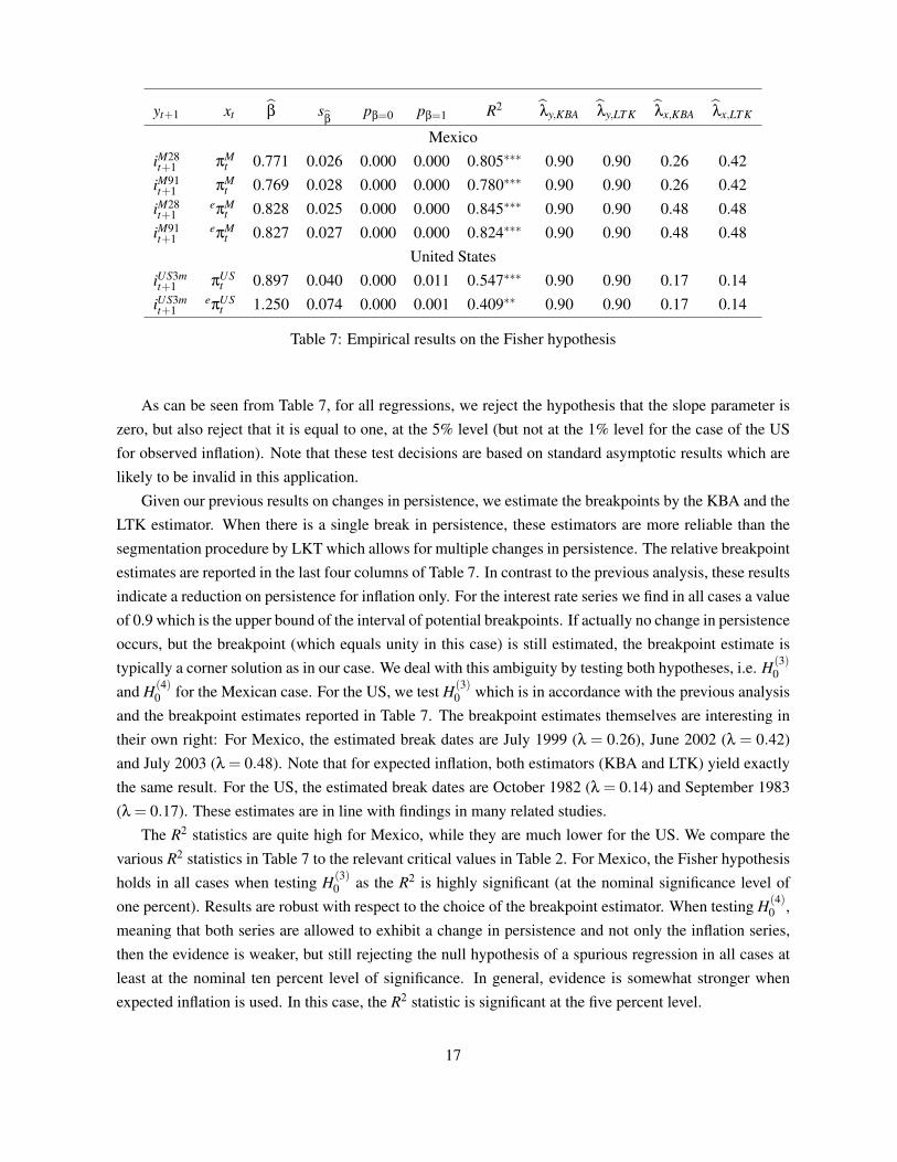
Table 7: Empirical results on the Fisher hypothesis
As can be seen from Table 7, for all regressions, we reject the hypothesis that the slope parameter iszero, but also reject that it is equal to one, at the 5% level (but not at the 1% level for the case of the USfor observed inflation). Note that these test decisions are based on standard asymptotic results which arelikely to be invalid in this application.
Given our previous results on changes in persistence, we estimate the breakpoints by the KBA and theLTK estimator. When there is a single break in persistence, these estimators are more reliable than thesegmentation procedure by LKT which allows for multiple changes in persistence. The relative breakpointestimates are reported in the last four columns of Table 7. In contrast to the previous analysis, these resultsindicate a reduction on persistence for inflation only. For the interest rate series we find in all cases a valueof 0.9 which is the upper bound of the interval of potential breakpoints. If actually no change in persistenceoccurs, but the breakpoint (which equals unity in this case) is still estimated, the breakpoint estimate istypically a corner solution as in our case. We deal with this ambiguity by testing both hypotheses, i.e. H(3)
0
and H(4)0 for the Mexican case. For the US, we test H(3)
0 which is in accordance with the previous analysisand the breakpoint estimates reported in Table 7. The breakpoint estimates themselves are interesting intheir own right: For Mexico, the estimated break dates are July 1999 (λ = 0.26), June 2002 (λ = 0.42)and July 2003 (λ = 0.48). Note that for expected inflation, both estimators (KBA and LTK) yield exactlythe same result. For the US, the estimated break dates are October 1982 (λ = 0.14) and September 1983(λ = 0.17). These estimates are in line with findings in many related studies.
The R2 statistics are quite high for Mexico, while they are much lower for the US. We compare thevarious R2 statistics in Table 7 to the relevant critical values in Table 2. For Mexico, the Fisher hypothesisholds in all cases when testing H(3)
0 as the R2 is highly significant (at the nominal significance level ofone percent). Results are robust with respect to the choice of the breakpoint estimator. When testing H(4)
0 ,meaning that both series are allowed to exhibit a change in persistence and not only the inflation series,then the evidence is weaker, but still rejecting the null hypothesis of a spurious regression in all cases atleast at the nominal ten percent level of significance. In general, evidence is somewhat stronger whenexpected inflation is used. In this case, the R2 statistic is significant at the five percent level.
17
Results for the US indicate clear rejections of the null hypothesis, too. When using the actual inflationseries, the null hypothesis is rejected at the one percent level. Evidence is a bit lower when expectedinflation is used, contrary to the Mexican case. Results are robust with respect to the particular breakpointestimator in use.
5 Concluding remarks
The contribution of this paper is threefold: (i) We extend the results within the spurious inference literatureby studying the estimates of a regression under shifting persistence variables. The results of such anextension are in line with (and similar to) those related to independent and integrated to the order onevariables studied by Phillips in the late Eighties. (ii) We propose a test procedure that distinguishesbetween spurious regressions and genuine ones, something that cannot be done, neither by cointegrationanalysis (when the variables are not known to exhibit a change in persistence), nor by classical statisticalinference, chiefly t- and F - test statistics. Monte Carlo experiments demonstrate that the test performswell in small samples, and when the breakpoints are unknown, both under the null and the alternative.Moreover, it is quite robust to mispecification of the number of series with breaks which is encouragingfor applied work. (iii) We apply our test statistic to the Fisher hypothesis for the U.S. and the Mexicancase. Contrary to the usual rejection of the hypothesis (using cointegration techniques), our test offersstrong evidence concerning the validity of the Fisher hypothesis.
References
BARSKY, R. B. (1987): “The Fisher hypothesis and the forecastability and persistence of inflation,”Journal of Monetary Economics, 19(1), 3–24.
BUSETTI, F., AND A. TAYLOR (2004): “Tests of stationarity against a change in persistence,” Journal ofEconometrics, 123(1), 33–66.
CHRISTOPOULOS, D. K., AND M. A. LEON-LEDESMA (2007): “A Long-Run Non-Linear Approach tothe Fisher Effect,” Journal of Money, Credit and Banking, 39(2-3), 543–559.
ENTORF, H. (1997): “Random Walks With Drifts: Nonsense Regression and Spurious Fixed-Effect Esti-mation,” Journal of Econometrics, 80, 287–296.
GARCIA, R., AND P. PERRON (1996): “An Analysis of the Real Interest Rate Under Regime Shifts,” TheReview of Economics and Statistics, 78(1), 111–125.
GRANGER, C., N. HYUNG, AND Y. JEON (2001): “Spurious regressions with stationary series,” AppliedEconomics, 33(7), 899–904.
GRANGER, C., AND P. NEWBOLD (1974): “Spurious Regressions in Econometrics,” Journal of Econo-metrics, 2, 11–20.
18
HALUNGA, A., D. R. OSBORN, AND M. SENSIER (2008): “Changes in the order of integration of USand UK inflation,” Economics Letters, 102, 30–32.
HARVEY, D., S. LEYBOURNE, AND A. TAYLOR (2006): “Modified tests for a change in persistence,”Journal of Econometrics, 134(2), 441–469.
HASSLER, U., AND J. SCHEITHAUER (2011): “Detecting changes from short to long memory,” StatisticalPapers, 52, 847–870.
HAUG, A., A. BEYER, AND W. DEWALD (2011): “Structural Breaks and the Fisher Effect,” The BEJournal of Macroeconomics, 11(1).
JENSEN, M. J. (2009): “The Long-Run Fisher Effect: Can It Be Tested?,” Journal of Money, Credit andBanking, 41(1), 221–231.
KANG, K. H., C.-J. KIM, AND J. MORLEY (2009): “Changes in US inflation persistence,” Studies inNonlinear Dynamics & Econometrics, 13(4), 1–21.
KEJRIWAL, M. (2012): “The Nature of Persistence in Euro Area Inflation: A Reconsideration,” mimeo.
KIM, J. (2000): “Detection of change in persistence of a linear time series,” Journal of Econometrics,95(1), 97–116.
KIM, J., J. BELAIRE FRANCH, AND R. BADILLI AMADOR (2002): “Corrigendum to Detection ofChange in Persistence of a Linear Time Series,” Journal of Econometrics, 109, 389–392.
KOURETAS, G. P., AND M. E. WOHAR (2012): “The dynamics of inflation: a study of a large number ofcountries,” Applied Economics, 44(16), 2001–2026.
KOUSTAS, Z., AND A. SERLETIS (1999): “On the Fisher effect,” Journal of Monetary Economics, 44(1),105–130.
KUMAR, M. S., AND T. OKIMOTO (2007): “Dynamics of persistence in international inflation rates,”Journal of Money, Credit and Banking, 39(6), 1457–1479.
KUROZUMI, E. (2005): “Detection of Structural Change in the Long-run Persistence in a Univariate TimeSeries,” Oxford Bulletin of Economics and Statistics, 67(2), 181–206.
LAI, K. S. (2008): “The puzzling unit root in the real interest rate and its inconsistency with intertemporalconsumption behavior,” Journal of International Money and Finance, 27(1), 140–155.
LANNE, M. (2006): “Nonlinear dynamics of interest rate and inflation,” Journal of Applied Econometrics,21(8), 1157–1168.
LEYBOURNE, S., T. KIM, AND A. TAYLOR (2007): “Detecting multiple changes in persistence,” Studiesin Nonlinear Dynamics & Econometrics, 11(3), 1370–1370.
19
LEYBOURNE, S., T.-H. KIM, V. SMITH, AND P. NEWBOLD (2003): “Tests for a change in persistenceagainst the null of difference-stationarity,” The Econometrics Journal, 6(2), 291–311.
LEYBOURNE, S., R. TAYLOR, AND T.-H. KIM (2007): “CUSUM of Squares-Based Tests for a Changein Persistence,” Journal of Time Series Analysis, 28(3), 408–433.
MALLIAROPULOS, D. (2000): “A note on nonstationarity, structural breaks, and the Fisher effect,” Jour-nal of Banking & Finance, 24(5), 695–707.
MARMOL, F. (1995): “Spurious Regressions Between I(d) Processes,” Journal of Time Series Analysis,16, 313–321.
MARMOL, F. (1996): “Nonsense Regressions between Integrated Processes of Different Orders.,” OxfordBulletin of Economics & Statistics, 58(3), 525–36.
MARMOL, F. (1998): “Spurious Regression Theory with Nonstationary Fractionally Integrated Pro-cesses,” Journal of Econometrics, 84, 233–250.
NEELY, C. J., AND D. E. RAPACH (2008): “Real interest rate persistence: evidence and implications,”Federal Reserve Bank of St. Louis Working Paper Series.
NORIEGA, A., C. CAPISTRAN, AND M. RAMOS-FRANCIA (2012): “On the dynamics of inflation per-sistence around the world,” Empirical Economics, pp. 1–23.
NORIEGA, A., AND M. RAMOS-FRANCIA (2009): “The dynamics of persistence in US inflation,” Eco-nomics Letters, 105(2), 168–172.
NORIEGA, A., AND D. VENTOSA-SANTAULARIA (2007): “Spurious Regression And Trending Vari-ables,” Oxford Bulletin of Economics and Statistics, 7, 4–7.
O’REILLY, G., AND K. WHELAN (2005): “Has euro-area inflation persistence changed over time?,”Review of Economics and Statistics, 87(4), 709–720.
PERRON, P. (2006): “Dealing with structural breaks,” Palgrave Handbook of Econometrics, 1, 278–352.
PHILLIPS, P. (1986): “Understanding Spurious Regressions in Econometrics,” Journal of Econometrics,33, 311–340.
(2005): “Econometric analysis of Fisher’s equation,” American Journal of Economics and Soci-ology, 64(1), 125–168.
RAPACH, D. E., AND C. E. WEBER (2004): “Are real interest rates really nonstationary? New evidencefrom tests with good size and power,” Journal of Macroeconomics, 26(3), 409–430.
RAPACH, D. E., AND M. E. WOHAR (2005): “Regime changes in international real interest rates: Arethey a monetary phenomenon?,” Journal of Money, Credit, and Banking, 37(5), 887–906.
20
ROSE, A. K. (1988): “Is the real interest rate stable?,” The Journal of Finance, 43(5), 1095–1112.
TSAY, W., AND C. CHUNG (2000): “The spurious regression of fractionally integrated processes,” Journalof Econometrics, 96(1), 155–182.
TSONG, C.-C., AND C.-F. LEE (2013): “Quantile cointegration analysis of the Fisher hypothesis,” Jour-nal of Macroeconomics, 35, 186–198.
VENTOSA-SANTAULARIA, D. (2009): “Spurious regression,” Journal of Probability and Statistics, 2009,1–27.
WESTERLUND, J. (2008): “Panel cointegration tests of the Fisher effect,” Journal of Applied Economet-rics, 23(2), 193–233.
A Asymptotic calculations
We present the proof for case M4. All the remaining cases follow the same steps. Let xt and yt+1 begenerated by eqs. (2) and (3), where, δ = 0 and φ = 1 for t = 1,2, . . . , [λxT ] and δ 6= 0 and | φ |< 1 fort = [λxT ] + 1, . . . ,T , λx ∈ [0,1]. [λxT ] denotes the non-null integer of λxT . By solving these equationsrecursively, you get,
∑t+1i=1 ei, and Ix(·) and Iy(·) are indicator functions. The asymptotics of the R2 requires several prior
asymptotics results for the following objects: R2 = 1−∑ u2t+1/∑(yt+1− y)2; ∑ u2
t = ∑y2t+1 + α2T +
β2∑x2
t − 2α∑yt+1− 2β∑yt+1xt + 2αβ∑xt ; βde f= (α β)′ = (X ′X)−1Xy, where X = (x1 . . . xT )
′ and y =
(y2 . . . yT+1)′. The asymptotic properties of all the elements that appear on these expressions are well-
known (see (Phillips 1986), for instance):
T−32 ∑xt
D→∫
λx
0Wx (6)
T−32 ∑yt+1
D→∫
λy
0Wy (7)
T−2∑x2
tD→
∫λx
0(Wx)
2 (8)
T−2∑y2
t+1D→
∫λy
0(Wy)
2 (9)
T−2∑xtyt+1
D→∫
λI
0WxWy (10)
21
where λI = min(λx,λy). The remaining calculi, that is, replacing eqs. (6-10) in the formula of α, β, ∑ u2t ,
and R2, is straightforward, but cumbersome and tedious. The above expressions are equivalent to thosepresented in Phillips (1987); they only differ in the upper limit of the stochastic integrals (λx/λx/λI insteadof 1); therefore, the asymptotic expressions of the R2 vary in exactly the same manner. This statementcan be easily proved by obtaining the limit expressions using MathematicaT M. The Mathematica code isavailable upon request.
22
Research Papers 2013
2012-52: José Manuel Corcuera, Emil Hedevang, Mikko S. Pakkanen and Mark Podolskij: Asymptotic theory for Brownian semi-stationary processes with application to turbulence
2012-53: Rasmus Søndergaard Pedersen and Anders Rahbek: Multivariate Variance Targeting in the BEKK-GARCH Model
2012-54: Matthew T. Holt and Timo Teräsvirta: Global Hemispheric Temperature Trends and Co–Shifting: A Shifting Mean Vector Autoregressive Analysis
2012-55: Daniel J. Nordman, Helle Bunzel and Soumendra N. Lahiri: A Non-standard Empirical Likelihood for Time Series
2012-56: Robert F. Engle, Martin Klint Hansen and Asger Lunde: And Now, The Rest of the News: Volatility and Firm Specific News Arrival
2012-57: Jean Jacod and Mark Podolskij: A test for the rank of the volatility process: the random perturbation approach
2012-58: Tom Engsted and Thomas Q. Pedersen: Predicting returns and rent growth in the housing market using the rent-to-price ratio: Evidence from the OECD countries
2013-01: Mikko S. Pakkanen: Limit theorems for power variations of ambit fields driven by white noise
2013-02: Almut E. D. Veraart and Luitgard A. M. Veraart: Risk premia in energy markets
2013-03: Stefano Grassi and Paolo Santucci de Magistris: It’s all about volatility (of volatility): evidence from a two-factor stochastic volatility model
2013-04: Tom Engsted and Thomas Q. Pedersen: Housing market volatility in the OECD area: Evidence from VAR based return decompositions
2013-05: Søren Johansen and Bent Nielsen: Asymptotic analysis of the Forward Search
2013-06: Debopam Bhattacharya, Pascaline Dupasand Shin Kanaya: Estimating the Impact of Means-tested Subsidies under Treatment Externalities with Application to Anti-Malarial Bednets
2013-07: Sílvia Gonçalves, Ulrich Hounyo and Nour Meddahi: Bootstrap inference for pre-averaged realized volatility based on non-overlapping returns
2013-08: Katarzyna Lasak and Carlos Velasco: Fractional cointegration rank estimation
2013-09: Roberto Casarin, Stefano Grassi, Francesco Ravazzolo and Herman K. van Dijk: Parallel Sequential Monte Carlo for Efficient Density Combination: The Deco Matlab Toolbox
2013-10: Hendrik Kaufmann and Robinson Kruse: Bias-corrected estimation in potentially mildly explosive autoregressive models
2013-11: Robinson Kruse, Daniel Ventosa-Santaulària and Antonio E. Noriega: Changes in persistence, spurious regressions and the Fisher hypothesis