Thailand, located in Southeast Asia between 5 and20° N latitude and 97 to 106° E longitude, connectswith 2 large oceans: the Indian Ocean and the PacificOcean. The climate of Thailand is influenced byboth oceans via atmospheric–oceanic circulation.The average annual temperature ranges from 26.3to 28.0°C, with the maximum temperature in Aprilvarying from 31.6 to 33.6°C. The average annualrainfall is 1200 to 1600 mm (TMD 2010). The summer monsoon season caused by the southwest monsoonand the Inter Tropical Convergence Zone (ITCZ)lasts from mid-May to mid-October. The pre-mon-
soon season is influenced by the southwest monsoonand the ITCZ moving from the Indian Ocean to Thai-land in May and to central China in mid-June. Sub-sequently, the monsoon season is associated with theITCZ moving back to cover Thailand during Augustto October.
The major occupation in Thailand is agriculture,which is a rain-fed system. Therefore, severe socio -economic problems are caused by rainfall variabi -lity and extreme weather events, e.g. flooding anddrought. Several potential factors, including land usechange (Croke et al. 2004, Bronstert 2004), deforesta-tion (Kanae et al. 2001), and atmospheric variability,are responsible for the hydrological fluctuations in
Changes in summer monsoon rainfall in the UpperChao Phraya River Basin, Thailand
Nkrintra Singhrattna*, Mukand Singh Babel
Water Engineering and Management (WEM), Asian Institute of Technology (AIT) Klong Luang, Pathumthani, Thailand
ABSTRACT: We determined the effects of climate change on pre-monsoon (May-June-July: MJJ)and monsoon (August-September-October: ASO) season rainfall in the Upper Chao Phraya RiverBasin, Thailand, by downscaling surface rainfall from large-scale atmospheric variables, i.e. sur-face air temperature (SAT), sea level pressure (SLP), and zonal and meridional wind (u and v,respectively). The data were obtained from the Geophysical Fluid Dynamics Laboratory (GFDL)model and used as predictors in a modified k-nearest neighbor (k-nn) model. Under climatechange scenarios A2 and B2, during 2011–2100, the increasing trends of annual SAT over north-ern Thailand and the South China Sea vary from 1.65 to 3.47°C century–1. By the end of the 21stcentury, the annual SAT anomalies range from +2 to +10°C. The increasing trends of annual SLPover the Gulf of Thailand and northern Thailand range from 0.40 to 0.83 mb century–1. Dependingupon the regions and scenarios, increasing and decreasing trends of annual u and v wereobserved. From the modified k-nn model, the effects of climate change on MJJ and ASO rainfallindicate decreasing trends during 2011–2100 with a maximum decrease by 6.16 mm yr–1, corre-sponding to the ASO rainfall under Scenario B2. In terms of effects on the frequency of extremeevents, dry (wet) conditions during 2011–2100 showed a greater (lesser) chance of occurrencethan the climatology, with the exception of ASO rainfall under the Scenario A2, which showed agreater chance of being both dry and wet. With a probability >70%, dry MJJ and ASO conditionswill be observed more often than wet, especially the dry ASO under Scenario B2, which was predicted for the 55 yr from 2046 –2100.
Resale or republication not permitted without written consent of the publisher
Clim Res 49: 155–168, 2011
terms of intensity and frequency of extreme events.Increasing greenhouse gas concentrations, in partic-ular CO2, greatly influence global warming (Mitchell1989, Maslin 2007, NIC 2009, NASA 2010). Conse-quently, climate change is expected to occur due toincreasing global surface temperatures (UNEP 2003,Trenberth 2008). Since rainfall in Thailand showssignificant links to large-scale atmospheric variables(LSAVs), e.g. temperature and pressure (Chen &Yoon 2000, Singhrattna et al. 2005b), the changingclimate affects rainfall via atmospheric–oceanic cir-culations. The objective of this study was to deter-mine the effects of climate change on summer mon-soon season rainfall in the Upper Chao Phraya RiverBasin (Thailand). Rainfall simulation by a stochasticstatistical model is a tool for long-term planning inwater resources and an adaptation strategy to dealwith future climate change.
2. METHODS
Based on the significant relationships betweenlocal hydroclimates (e.g. precipitation) and LSAVs(e.g. sea level pressure), LSAVs have been used aspredictors in multiple regressions to forecast hydro-climates (Hamlet et al. 2002, McCabe & Dettinger2002, Singhrattna et al. 2005a, Koocheki et al. 2006,Mo riondo & Bindi 2006). Moreover, with an assump-tion that general circulation models (GCMs) simulateatmospheric variables in the upper air level, e.g. tem-perature and pressure, more reliably than surfacevariables, e.g. precipitation, regressions incorporat-ing LSAVs are also applied to downscale regionaland local surface hydroclimates from variables in theupper air level. The GCM outcomes are the fore-casted future climate, which is expected to changerelative to future environmental systems and humanactivities. GCMs provide projected data of LSAVsunder several climate change scenarios proposedby the Intergovernmental Panel on Climate Change(IPCC). The proposed scenarios incorporate differ-ences in socioeconomic, demographic, and techno-logical growth and environmental changes such asgreenhouse gas concentrations, in particular CO2.The model resolution in terms of spatial gridded cov-erage varies from 2.8° longitude × 2.8° latitude to 5.6°longitude × 5.6° latitude. The length of data seriesranges series from 100 to 211 yr (see also IPCC 2001).
In terms of regression analysis, although paramet-ric approaches, e.g. linear regression, have beenwidely applied due to their simplicity, there are somedrawbacks of fitting a regression by parametric
approaches, such as a prior assumption of relation-ships between dependent and independent variablesand a method of global fitting. Therefore, nonpara-metric approaches were developed and adopted toimprove the fitting performance. Without a prior as -sumption, the fitting functions of nonparametric ap -proaches can locally capture the relationships be -tween dependent and independent variables or fitthe regression at a given point by a small set ofneighbors. Hence, the nonparametric approaches areflexible and able to fit any arbitrary, e.g. bivariateand multivariate data. There are several approachesof nonparametric regression. One that was devel-oped to capture the discontinuities of the derivativecurve is the spline approach. Another approach thatapplies a regression locally to a given point andits neighbors is called ‘local polynomials.’ This ap -proach includes locally weighted polynomials (Loader1999) and k-nearest neighbor (k-nn) local polynomi-als (Owosina 1992, Rajagopalan & Lall 1999). In thisstudy, aiming to determine the effects of climatechange and downscale rainfall from LSAVs of aGCM, the modified k-nn model was adopted to fit theregression between summer monsoon season rainfalland identified atmospheric predictors.
2.1. Study area
There are 25 major river basins in Thailand. Thelargest basin is the Chao Phraya River Basin, whichis located in central Thailand and covers an area of178 000 km2, i.e. 35% of the country’s land area. TheUpper Chao Phraya River consists of 4 tributaries:Ping, Wang, Yom, and Nan Rivers. Our study area,i.e. the Ping River Basin, covers a drainage area of33 899 km2 with a river length of 740 km originatingin northern Thailand (Fig. 1). The irrigated area ofthe study basin covers 2332 km2. Although the basinreceives a sufficient runoff of 8700 million m3 (MCM)yr–1 for an average annual demand of 6127 MCM,water shortage especially in the upstream region isevident during the dry season. An average annualinflow of 5900 MCM from the Ping River Basin isstored in a reservoir of the Bhumipol Dam locateddownstream of the Ping River. The Bhumipol Damwas constructed for the purposes of hydropower pro-duction, agricultures, fishery, transportation, andflood mitigation. The maximum storage capacity is13 462 MCM with a hydro power capacity of 780 MW.The dam regulates and supplies water to the down-stream area, e.g. the Lower Chao Phraya River Basin,which has an irrigated area of 6878 km2. The domes-
156
Singhrattna & Singh Babel: Changes in Thailand summer monsoon rainfall
tic and total water demand in the Chao Phraya RiverBasin is estimated to be 2240 and 11 000 MCM yr–1,re spec tively. The water management and planningof the Ping River Basin influence the socioeconomicsof this basin and downstream areas. Hence, the PingRiver Basin was selected to investigate the effects ofclimate change on rainfall, with the aim of develop-ing a sustainable plan for water resource use.
2.2. Data
2.2.1. Observed data
Data on daily rainfall from 1950–2007 were ob -tained from 50 selected stations located in and aroundthe Ping River Basin (Fig. 2). All stations wereselected based on the length of time series andwhether incomplete data represented less than 5%of the 30 recent years of data. The data of all 50 sta-tions were provided by the Royal Irrigation Depart-ment of Thailand, the Thailand Meteoro logical De -partment, and the Department of Water Resources.Because the monthly rainfall from 1950–2007 of all 50
selected stations was significantly correlated at the 95% confidence levelby Fisher’s transformation (Haan2002), with the correlation coefficientsranging from 0.46 to 0.96, the monthlyrainfall was averaged over the 50selected stations. The annual cycle ofrainfall (Fig. 3) has 2 peaks influencedby the southwest monsoon and theITCZ. The secondary peak is foundduring May-June-July (MJJ), i.e. thepre-monsoon season, during which thesouthwest monsoon and the ITCZbring moisture from the Indian Oceanto Thailand, and subsequently to theSouth China Sea and central China.The primary peak during August-Sep-tember-October (ASO) correspondingto the monsoon season rainfall iscaused by the ITCZ moving back toThailand. As a result, the pre-monsoonand monsoon season rainfall are thesums of rainfall during MJJ and ASO,respectively.
157
Fig. 1. (a) Thailand and (b) UpperChao Phraya River Basin: Ping, Wang,
Yom, and Nan River Basins
Fig. 2. Rainfall stations in and around the Ping River Basin, Thailand
Clim Res 49: 155–168, 2011
In terms of LSAVs, 4 principal variables, i.e. surfaceair temperature (SAT), sea level pressure (SLP), sur-face zonal wind (u), and surface meridional wind (v)were used as the independent variables or predictorsof the pre-monsoon (MJJ) and monsoon (ASO) sea-son rainfall in a multivariate regression (Singhrattnaet al. in press). Based on significant correlations atthe 95% confidence level between rainfall (duringMJJ and ASO) and 4 LSAVs, the spatial coverage(Table 1) of 4 predictors was identified by cross-correlation maps (Grantz et al. 2005, Schöngart &Junk 2007). The correlation maps are the interactiveplots and analysis provided by the Earth SystemResearch Laboratory (ESRL) of the National OceanicAtmo spheric Administration (NOAA; ESRL 2008).The nonlinear temporal relationships between rain-fall and LSAVs are ob served from the correlationmaps. Few significant correlations were found dur-ing 1950–2007; however, the relationships devel-oped after 1980 were significant at the 95% confi-dence level. The nonlinear interdecadal relationshipsare influenced by the subsidence of the Walker circu-lation on Thailand and Southeast Asia after 1980,which are associated with the shifting regions of seasurface temperature anomalies in the Pacific Ocean(Krishna Kumar et al. 1995, Singhrattna et al. 2005b).Corresponding to the identified regions of predictorsby the correlation maps, the observed LSAVs used inthis study were obtained from the reanalysis deriveddata (Kalnay et al. 1996) of the National Centers
for Environmental Prediction (NCEP/ NOAA). With agrid resolution of 2.5° longitude × 2.5° latitude, themonthly means from 1948–2007 of 4 variables aver-aged over the identified regions were used to deter-mine the variability of predictors.
2.2.2. GCM data and climate change scenarios
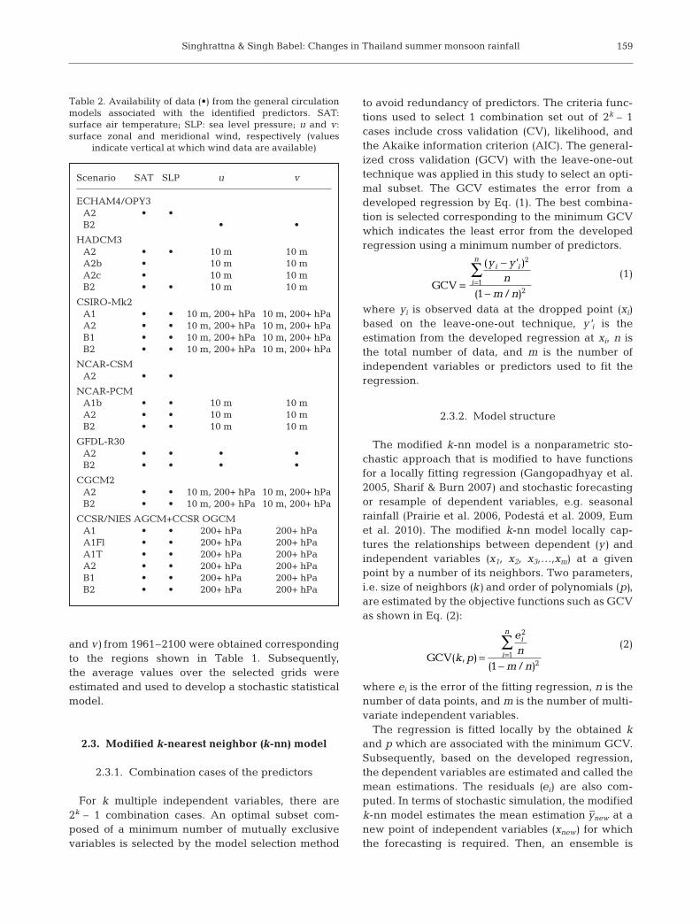
The GCM data used in this study are presentedin the IPCC Third As sessment Report (TAR; IPCC2001). The GCM selection was based on the avail-ability of all 4 predictors. From Table 2, we selected amodel of the Geophysical Fluid Dynamics Laboratory(GFDL), namely GFDL-R30, which provides simu-lated data of all identified predictors. The GFDL-R30is a coupled atmosphere–ocean general circulationmodel (AOGCM), in which the atmo spheric compo-nent covers 7680 grids with a gridded resolution of3.75° longitude × 2.25° latitude, and it has 14 verticallevels. The ocean component has 196 × 80 globalgrids of horizontal resolution (i.e. 3.75° longitude ×1.125° latitude) and 18 spaced vertical levels (Del-worth et al. 2002). The model simulates conditions ofdoubling atmospheric CO2 by 2100. The griddeddata of GFDL-R30 available from 1961–2100 are pro-vided by the IPCC Data Distribution Centre (IPCC-DDC 2009). To determine the effects of climatechange on pre-monsoon (MJJ) and monsoon (ASO)season rainfall in the study basin, the gridded data ofpredictors simulated by GFDL-R30 under 2 IPCCemission scenarios, i.e. A2 and B2, were used. Themonthly gridded data of 4 predictors (i.e. SAT, SLP, u,
158
0
50
100
150
200
250
Rain
fall
(mm
)
J F M A M J J A S O N D
Fig. 3. Annual cycle of mean monthly rainfall averaged over 50 selected stations during 1950–2007
Predictor Region Identified region °N °E
MJJ rainfall SAT Northern Thailand 20.0 97.5–102.5SLP Gulf of Thailand 7.5–10.0 102.5–107.5u Equatorial Indian 0 82.5–87.5 Oceanv Eastern equatorial 0–2.5 172.5–175.0 Pacific Ocean
ASO rainfall SAT South China Sea 2.5–5.0 107.5–110.0SLP Northern Thailand 17.5–20.0 97.5–100.0u Gulf of Thailand 10.0 100.0–102.5v Andaman Sea 10.0 95.0–97.5
Table 1. Identified predictors of May-June-July (MJJ) and August-September-October (ASO) rainfall by the correlationmaps. SAT: surface air temperature T; SLP: sea level pressureT; u and v: surface zonal and meridional wind, respectively
Singhrattna & Singh Babel: Changes in Thailand summer monsoon rainfall
and v) from 1961–2100 were obtained correspondingto the regions shown in Table 1. Subsequently,the average values over the selected grids were estimated and used to develop a stochastic statisticalmodel.
2.3. Modified k-nearest neighbor (k-nn) model
2.3.1. Combination cases of the predictors
For k multiple independent variables, there are 2k – 1 combination cases. An optimal subset com-posed of a minimum number of mutually exclusivevariables is selected by the model selection method
to avoid redundancy of predictors. The criteria func-tions used to select 1 combination set out of 2k – 1cases include cross validation (CV), likelihood, andthe Akaike information criterion (AIC). The general-ized cross validation (GCV) with the leave-one-outtechnique was applied in this study to select an opti-mal subset. The GCV estimates the error from adeveloped regression by Eq. (1). The best combina-tion is selected corresponding to the minimum GCVwhich indicates the least error from the developedregression using a minimum number of predictors.
(1)
where yi is observed data at the dropped point (xi)based on the leave-one-out technique, y ’i is the estimation from the developed regression at xi, n isthe total number of data, and m is the number ofindependent variables or predictors used to fit theregression.
2.3.2. Model structure
The modified k-nn model is a nonparametric sto-chastic approach that is modified to have functionsfor a locally fitting regression (Gangopadhyay et al.2005, Sharif & Burn 2007) and stochastic forecastingor resample of dependent variables, e.g. seasonalrainfall (Prairie et al. 2006, Podestá et al. 2009, Eumet al. 2010). The modified k-nn model locally cap-tures the relationships between dependent (y) andindependent variables (x1, x2, x3,…,xm) at a givenpoint by a number of its neighbors. Two parameters,i.e. size of neighbors (k) and order of polynomials (p),are estimated by the objective functions such as GCVas shown in Eq. (2):
(2)
where ei is the error of the fitting regression, n is thenumber of data points, and m is the number of multi-variate independent variables.
The regression is fitted locally by the obtained kand p which are associated with the minimum GCV.Subsequently, based on the developed regression,the dependent variables are estimated and called themean estimations. The residuals (ei) are also com-puted. In terms of stochastic simulation, the modifiedk-nn model estimates the mean estimation –ynew at anew point of independent variables (xnew) for whichthe forecasting is required. Then, an ensemble is
GCV
’
=
−
−=∑ ( )
( / )
y yn
m n
i i
i
n 2
121
GCV( , )( / )
k p
en
m n
i
i
n
=−
=∑
2
121
159
Scenario SAT SLP u v
ECHAM4/OPY3A2 • •B2 • •
HADCM3A2 • • 10 m 10 mA2b • 10 m 10 mA2c • 10 m 10 mB2 • • 10 m 10 m
CSIRO-Mk2A1 • • 10 m, 200+ hPa 10 m, 200+ hPaA2 • • 10 m, 200+ hPa 10 m, 200+ hPaB1 • • 10 m, 200+ hPa 10 m, 200+ hPaB2 • • 10 m, 200+ hPa 10 m, 200+ hPa
NCAR-CSMA2 • •
NCAR-PCMA1b • • 10 m 10 mA2 • • 10 m 10 mB2 • • 10 m 10 m
GFDL-R30A2 • • • •B2 • • • •
CGCM2A2 • • 10 m, 200+ hPa 10 m, 200+ hPaB2 • • 10 m, 200+ hPa 10 m, 200+ hPa
Table 2. Availability of data (•) from the general circulationmodels associated with the identified predictors. SAT: surface air temperature; SLP: sea level pressure; u and v:surface zonal and meridional wind, respectively (values
indicate vertical at which wind data are available)
Clim Res 49: 155–168, 2011
obtained by adding a residual (ei) to –ynew. A residualis ran domly selected from the k-nearest neighbors ofxnew, where k is the size of neighbors that can be dif-ferent from k for the fitting regression. In practice, kis estimated by 12222n – 1. The random selection of resid-uals applies a weight function as shown in Eq. (3),which gives less weight to the farthest neighbor andmore weight to the nearest neighbor.
(3)
where W( j) is the weight value of a neighbor of xnew
where the distance between xnew and this neighborfalls in the j th rank.
The distance (d) from a neighbor to xnew is calcu-lated by the Euclidean distance as shown in Eq. (4).
(4)
where i = 1, 2, 3,…, n, and m is the number of multi-variate independent variables.
By repeating the random selection of residuals, Nsimulating ensembles at a forecasting point areobtained, e.g. in this case 300 en sembles each of MJJand ASO rainfall in a simulation year.
The fitting regression from the modified k-nn modeldeveloped to capture the relationships between sum-mer monsoon rainfall during MJJ and ASO in thePing River Basin and predictors (i.e. SAT, SLP, uand v) using GFDL-R30 data from 1961–2007 underclimate change scenarios is assumed to be valid forrecent climate and future changing climate.
2.3.3. Model evaluation
The leave-one-out cross validation was appliedto evaluate the performance of the modified k-nnmodel. Based on this technique, an observation isremoved from the data sets of dependent and inde-pendent variables. The regression is then fittedusing the remaining data as the training set. At theeliminated point, the estimation is calculated bythe developed regression and compared to the ob -served data. The validation was applied to allpoints of data from 1961–2007. It was also doneseparately for each season (MJJ and ASO) and sce-nario (A2 and B2). Furthermore, 2 criteria adoptedto evaluate the modified k-nn model included thecorrelation coefficient (r) and likelihood skill score(LLH). The correlation coefficient can measure alinear correlation between ob servations and simu-
lations. For a given year, the median rainfall wasestimated from 300 rainfall ensembles whichwere obtained from the modified k-nn model. Sub-sequently, the correlation between observed andmodeled rainfall during 1961–2007 was calculated.The significant level of correlation is estimated byFisher’s transformation (z ’; Haan 2002) as shown inEq. (5). The distribution of correlations, which maynot follow a Gaussian distribution, is converted to anormal distribution using z ’. The value of z ’ is thenused to compare to z of the standard normal dis -tribution to obtain the significance level (p) of acorrelation coefficient.
(5)
In terms of LLH, the likelihood can evaluate amodel on capturing the probability density function(PDF) of the observations. The first step of LLHcalculation is to divide the climatological datainto 3 categories, i.e. in this case at the 33rd and67th percentiles. Rainfall below the 33rd percentilewas de fined as below-normal rainfall, whereasrainfall above the 67th percentile was considered above-normal rainfall. The categorical probabilitiesof historical data in each category are thus 1/3.Subsequently, from the modified k-nn model, theN ensembles in a given year (i.e. 300 ensembles inthis case) were divided into 3 categories at thesame thresholds of climatology. The categoricalprob abilities of ensembles in a given year, whichare the proportion of ensemble members fallingin each category, were computed separately foreach season of rainfall and each year from 1961–2007. LLH of a given year was estimated as perEq. (6):
(6)
where n is the number of years, j is the category of anobservation in Year t, P̂j,t is the probability of ensem-bles for Category j in Year t; P̂j,t = (P̂l,t, P̂2,t, P̂3,t,…, P̂k,t),for which k is the number of categories (i.e. 3),and Pcj,t is the climatology probability of Category jin Year t.
The LLH ranges from 0.0 to +3.0, which is thenumber of categories. The value of 0.0 indicates anin ability to capture the PDF of the observation,whereas a value greater than +1.0 indicates a betterperformance than climatology. Perfect performanceof the model is shown by a score of +3.0.
zrr
’ . ln= +−
0 511
W jj
ii
k( )
/
( / )
=
=∑
1
11
d x xi new j i jj
m
= −=∑( ), ,
2
1
LLH = =
=
∏
∏
ˆ,
,
P
P
j tt
n
cj tt
n1
1
160
Singhrattna & Singh Babel: Changes in Thailand summer monsoon rainfall
2.3.4. Probability density function
The PDF can be developed from Nensembles simulated by the modifiedk-nn model. Non-exceedence andexceedence probabilities of extremeevents, e.g. dry and wet, are then esti-mated from the PDF based on thedefined thresholds of events. The prob-abilities of extreme events are a usefultool in decision making to managewater resources, plan agriculturalpractices, operate reservoirs, anddevelop insurance policies. In this case,dry conditions of MJJ (ASO) rainfallwere defined as rainfall below the 20thpercentile, i.e. 381.7 (498.2) mm, whichwas estimated by the observed MJJ(ASO) rainfall during 1950–2007. Onthe other hand, wet conditions of MJJ(ASO) rainfall were defined as rainfallabove the 80th percentile, i.e. 528.9(624.8) mm. The rainfall that did notfall into either category was denoted asnormal. The effects of climate changeon pre-monsoon (MJJ) and monsoon(ASO) season rainfall in the Ping RiverBasin during 2011–2100 are presentedin terms of dry and wet occurrencealong with the non-exceedence andexceedence probabilities of events.
3. RESULTS AND DISCUSSION
3.1. Characteristics of the GFDL-R30
3.1.1. Performance
The performance of GFDL-R30 was evaluated bythe following statistical criteria: mean (x), and stan-dard de viation (SD), coefficient of determination (R2),and normalized root mean square error (NRMSE).The monthly observed data of identified predictorsfrom NCEP/NOAA and modeled data obtained fromGFDL-R30 during 1961–2007 were used to estimateall criteria. From Fig. 4a, the GFDL-R30 under A2 andB2 was unable to capture the x of observed SAT, SLP,u, and v, with the exception of the x of v, which is as-sociated with the ASO rainfall predictor. The x of ob-served v from 1961–2007 was estimated as 0.64 m s–1,whereas the x of modeled v under A2 (B2) was calcu-lated as 0.68 (0.66) m s–1, which falls into the 95% con -
fidence intervals (CI) for x of the observed v. In termsof SD (Fig. 4b), only the SD of modeled SLP corre-sponding to the predictors of MJJ rainfall fell into the95% CI for SD of the 1961–2007 ob served SLP. Fig. 5shows the R2 between observed and simulated pre-
161
ASOMJJ
Season of rainfall
21
22
23
24
25
26
27
28
29
30
31
SA
T (°C
)
SL
P (m
b)
u (m
s–1
)
v (m
s–1
)
SA
T (°C
)
SL
P (m
b)
u (m
s–1
)
v (m
s–1
)
OBSR30 (A2)R30 (B2)
ASOMJJ960
970
980
990
1000
1010
ASOMJJ–1.0
– 0.5
0.0
0.5
1.0
1.5
2.0
ASOMJJ–1.5
–1.0
– 0.5
0.0
0.5
1.0(a)
ASOMJJ0
1
2
3
4
5
6
ASOMJJ1.0
1.5
2.0
2.5
3.0
3.5
4.0
4.5
5.0
5.5
OBSR30 (A2)R30 (B2)
ASOMJJ1.0
1.5
2.0
2.5
3.0
3.5
4.0
4.5
ASOMJJ
1.0
1.5
2.0
2.5
3.0
3.5
4.0(b)
Fig. 4. Statistics of the observed and GFDL-R30 predictors of May-June-July(MJJ) and August-September-October (ASO) rainfall: (a) mean (x ) and (b)SD; the 95% confidence intervals for x and SD are presented by the verticallines extending from the x and SD of climatology. SAT: surface air tem -perature; SLP: sea level pressure; u and v: surface zonal and meridional
winds, respectively
ASOMJJ
Season of rainfall
0
0.1
0.2
0.3
0.4
0.5
0.6
0.7
0.8
R2
SATSLPuv
ASOMJJ0
0.1
0.2
0.3
0.4
0.5
0.6
0.7
0.8(a) (b)
Fig. 5. R2 between observed and GFDL-R30 predictorsof May-June-July (MJJ) and August-September-October(ASO) rainfall, under the (a) A2 and (b) B2 scenarios. SAT:surface air temperature; SLP: sea level pressure; u and v :
surface zonal and meridional winds, respectively
Clim Res 49: 155–168, 2011
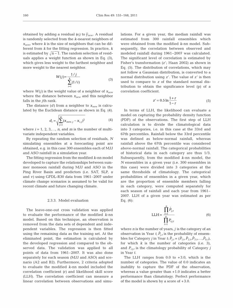
dictors obtained from GFDL-R30.Comparing between R2 associatedwith the MJJ and ASO rainfall predic-tors, the greater R2 correspond to all 4predictors of ASO rainfall. Hence,based on the R2, better performance ofGFDL-R30 was observed in the ASOrainfall predictors under both scenar-ios of climate change. According toA2 (B2), 70–78% (67–78%) of the ob-served data of ASO rainfall predictorscan be explained by the modeled re-sults from GFDL-R30. As expected,the NRMSEs were consistent with theR2, except the NRMSE of SLP. TheNRMSEs of SAT, u, and v under A2(Fig. 6a), varying from 0.16 to 0.49,correspond to the ASO rainfall predic-tors, which were slightly lower thanthose of the MJJ rainfall predictors.Moreover, from Fig. 6b, the NRMSEswith respect to B2 were consistentwith A2, except the NRMSE of v.
3.1.2. Annual variability and trendsin LSAVs
The variability of LSAVs used aspredictors of MJJ and ASO rainfallwas determined by the observed datafrom 1948–2007 provided by NCEPand the projected data from 2011–2100 simulated by GFDL-R30 under
A2 and B2 scenarios. For the predictors of MJJ rain-fall, the annual observed SAT anomalies (Fig. 7),which were estimated with respect to observed SATaveraged from 1961–1990, showed that the tem -peratures over northern Thailand (see also Table 1)during the 1990s were warmer than in the earliercentury. The annual observed SAT from 1948–2007tended to increase by 0.41°C century–1. It is lowerthan the trend in global surface temperatures, whichindicate a range of 1 to 2°C century–1 (IPCC 2007,Jenkins et al. 2008, Hansen et al. 2010). Moreover, bythe end of the 21st century, the GFDL model suggeststhat the SAT over this region will be 2 to 5°C warmerwith increasing trends of 3.47 and 1.93°C century–1
under A2 and B2, re spectively. Both trends were sig-nificant at the 99.9% confidence level by Student’s t-test (Haan 2002). The variability of temperature wasnot only observed in terms of magnitude but also
162
ASOMJJ
Season of rainfall
0.0
0.5
1.0
1.5
2.0
2.5
3.0
3.5N
RM
SE
NR
MS
E
SAT
SLP
uv
ASOMJJ
0.0
0.5
1.0
1.5
2.0
2.5
3.0
3.5(a) (b)
Fig. 6. Normalized root mean square error (NRMSE) fromGFDL-R30 predictions of May-June-July (MJJ) and August-September-October (ASO) rainfall, under the (a) A2 and (b)B2 scenarios. SAT: surface air temperature; SLP: sea levelpressure; u and v : surface zonal and meridional winds,
respectively
1940 1960 1980 2000 2020 2040 2060 2080 2100– 4
–2
0
2
4
An
nu
al v
ano
maly
(m
s–1
)
–4
–2
0
2
4
Annual u
ano
maly
(m
s–1
)
–4
–2
0
2
4
Annual S
LP
ano
maly
(m
b)
–6
–4
–2
0
2
4
6
Annual S
AT
ano
maly
(°C
)
Observed anomalies
5-year running mean (obs)
5-year running mean (A2)
5-year running mean (B2)
Fig. 7. Annual anomalies of 4 observed (1948–2007) predictors of May-June-July (MJJ) rainfall, and the 5 yr running mean from observed and GFDL-simu-lated (2011–2100) data; anomalies are estimated with respect to observed ormodel-simulated 1961–1990 average values. SAT: surface air temperature; SLP:
sea level pressure; u and v : surface zonal and meridional winds, respectively
Singhrattna & Singh Babel: Changes in Thailand summer monsoon rainfall
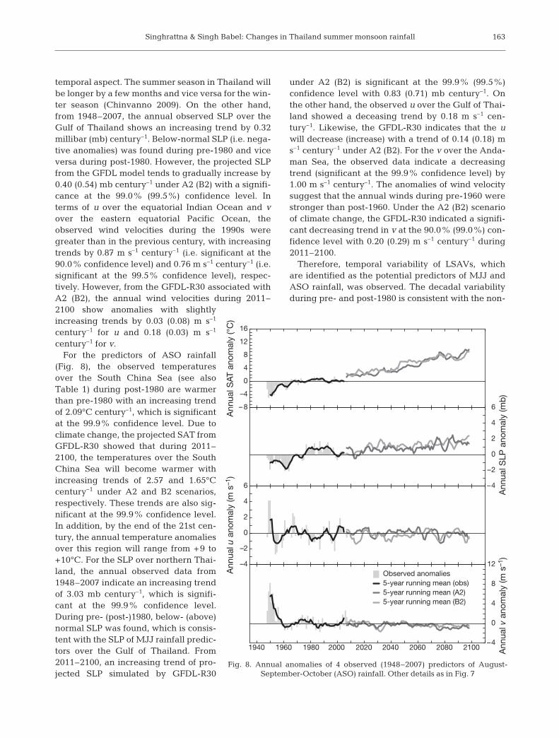
temporal aspect. The summer season in Thailand willbe longer by a few months and vice versa for the win-ter season (Chinvanno 2009). On the other hand,from 1948–2007, the annual observed SLP over theGulf of Thailand shows an increasing trend by 0.32millibar (mb) century–1. Below-normal SLP (i.e. nega-tive anomalies) was found during pre-1980 and viceversa during post-1980. However, the projected SLPfrom the GFDL model tends to gradually increase by0.40 (0.54) mb century–1 under A2 (B2) with a signifi-cance at the 99.0% (99.5%) confidence level. Interms of u over the equatorial Indian Ocean and vover the eastern equatorial Pacific Ocean, theobserved wind velocities during the 1990s weregreater than in the previous century, with increasingtrends by 0.87 m s–1 century–1 (i.e. significant at the90.0% confidence level) and 0.76 m s–1 century–1 (i.e.significant at the 99.5% confidence level), respec-tively. However, from the GFDL-R30 associated withA2 (B2), the annual wind velocities during 2011–2100 show anomalies with slightlyincreasing trends by 0.03 (0.08) m s–1
century–1 for u and 0.18 (0.03) m s–1
century–1 for v.For the predictors of ASO rainfall
(Fig. 8), the observed temperaturesover the South China Sea (see alsoTable 1) during post-1980 are warmerthan pre-1980 with an increasing trendof 2.09°C century–1, which is significantat the 99.9% confidence level. Due toclimate change, the projected SAT fromGFDL-R30 showed that during 2011–2100, the temperatures over the SouthChina Sea will become warmer withincreasing trends of 2.57 and 1.65°Ccentury–1 under A2 and B2 scenarios,respectively. These trends are also sig-nificant at the 99.9% confidence level.In addition, by the end of the 21st cen-tury, the annual temperature anomaliesover this region will range from +9 to+10°C. For the SLP over northern Thai-land, the annual observed data from1948–2007 indicate an increasing trendof 3.03 mb century–1, which is signifi-cant at the 99.9% confidence level.During pre- (post-)1980, below- (above)normal SLP was found, which is consis-tent with the SLP of MJJ rainfall predic-tors over the Gulf of Thailand. From2011–2100, an increasing trend of pro-jected SLP simulated by GFDL-R30
under A2 (B2) is significant at the 99.9% (99.5%)confidence level with 0.83 (0.71) mb century–1. Onthe other hand, the observed u over the Gulf of Thai-land showed a de ceasing trend by 0.18 m s–1 cen-tury–1. Likewise, the GFDL-R30 indicates that the uwill decrease (increase) with a trend of 0.14 (0.18) ms–1 century–1 under A2 (B2). For the v over the Anda -man Sea, the observed data indicate a decreasingtrend (significant at the 99.9% confidence level) by1.00 m s–1 century–1. The anomalies of wind velocitysuggest that the annual winds during pre-1960 werestron ger than post-1960. Under the A2 (B2) scenarioof climate change, the GFDL-R30 in dicated a signifi-cant de creasing trend in v at the 90.0% (99.0%) con-fidence level with 0.20 (0.29) m s–1 century–1 during2011–2100.
Therefore, temporal variability of LSAVs, whichare identified as the potential predictors of MJJ andASO rainfall, was observed. The decadal variabilityduring pre- and post-1980 is consistent with the non-
163
–4
0
4
8
12
Observed anomalies
5-year running mean (obs)
5-year running mean (A2)
5-year running mean (B2)
–4
–2
0
2
4
6 –4
–2
0
2
4
6– 8
–4
0
4
8
12
16
1940 1960 1980 2000 2020 2040 2060 2080 2100
An
nu
al v
an
om
aly
(m
s–1
)
An
nu
al u
an
om
aly
(m
s–1
)
An
nu
al S
LP
an
om
aly
(m
b)
An
nu
al S
AT
an
om
aly
(°C
)
Fig. 8. Annual anomalies of 4 observed (1948–2007) predictors of August-September-October (ASO) rainfall. Other details as in Fig. 7
Clim Res 49: 155–168, 2011164
linear relationships between LSAVs and summermonsoon rainfall which are found in the correla-tion maps (Singhrattna et al. in press). The decadal variability and the nonlinear relationships are alsocorroborated by Singhrattna et al. (2005b). Via theWalker circulation, temporal variability is influencedby the sea surface temperature anomalies, whichhave shifted from the dateline to the eastern equato-rial Pacific Ocean during recent decades. Due to climate change, the LSAVs also indicate annual variability and significant trends during 2011–2100.With significance at the 99.9% confidence level,the annual SAT tends to increase ranging from 1.65to 3.47°C century–1. The annual SLP also tends toincrease varying from 0.40 to 0.83 mb century–1.However, the trends of annual u and v are dependentupon the identified regions and scenarios of climatechange. By atmospheric-oceanic circulation, theeffects of climate change on the annual variability ofLSAVs may influence the fluctuations of rainfall andfrequencies of extreme events, i.e. dry and wet dur-ing pre-monsoon and monsoon seasons in the studybasin. Hence, based on the relationships betweenrainfall and identified LSAVs, the modified k-nnmodel was developed to determine the variability ofrainfall due to climate change.
3.2. Model performance of the modified k-nnmodel
3.2.1. Optimal combination cases of predictors
The GCV was adopted to select the optimal subsetsof predictors which consisted of mutually exclusiveindependent variables. With re spect to 4 identifiedpredictors each of MJJ and ASO rainfall, there were15 combination cases. The GCVs were estimatedseparately for MJJ and ASO rainfall predictors usingthe 1961–2007 simulated LSAVs by GFDL-R30 underA2 and B2 as the independent variables and the1961–2007 observed rainfall as the dependent vari-able. The GCV of each combination case was alsocalculated under a condition of varying lead periodsof predictors from 4 to 15 mo prior to the start of therainfall season. Based on the minimum GCV, a bestcombination case was se lected. Associated with A2,the optimal combination of MJJ (ASO) rainfall predictors consisted of the SLP and u (u and v) dur-ing November-December-January, NDJ (April-May-June, AMJ) which had a 6 (4) mo lead time. On theother hand, the selected subsets corresponding to B2are the SLP for MJJ rainfall predictors, and the SAT
and SLP for ASO rainfall predictors. The lead times ofpredictors were 6 and 14 mo, i.e. during NDJ andJune-July-August (JJA), respectively.
3.2.2. Model evaluation
The modified k-nn model was evaluated using cor-relation (r) and likelihood (LLH). With leave-one-outcross vali dation, all points of data from 1961–2007were used to evaluate the models for MJJ and ASOrainfall. The median rainfall in a given year was com-puted from 300 ensembles and subsequently used tocalculate the correlations. Under A2, the correlationbetween 1961– 2007 observed and modeled MJJ(ASO) rainfall was estimated at 0.41 (0.51), which issignificant at the 99.0% (99.9%) confidence level byFisher’s transformation. The median LLH from thesimulation of 1961–2007 MJJ rainfall was 1.12,whereas the median LLH from the simulation of ASOrainfall was 1.23. Hence, with respect to A2, the per-formance of the modified k-nn model in capturing thePDF of MJJ and ASO rainfall was better than that ofthe clima tology. On the other hand, the correlationbe tween observed and modeled MJJ rainfall corre-sponding to B2 was calculated to be 0.17. For ASOrainfall was better, the correlation was estimated to be0.38, which is significant at the 99.0% confidencelevel. Moreover, the median LLH associated with MJJ(ASO) rainfall was estimated as 1.12 (0.79). Therefore,under the B2 scenario, better performance in captur-ing the PDF of historical data compared to the clima-tology was found in the model for MJJ rainfall.
As a result, the modified k-nn model developed forMJJ rainfall under A2 (B2) used SLP and u (SLP) dur-ing NDJ as the predictors. At the 99.0% confidencelevel, the model under A2 indicated a significant cor-relation between observed and modeled MJJ rainfallduring 1961–2007. Furthermore, the models underboth scenarios of climate change captured the PDF ofobserved MJJ rainfall with LLH scores of 1.12, whichwas better than the climatology. On the other hand,the modified k-nn model with the predictors of u andv (SAT and SLP) during AMJ (JJA) was developed tosimulate the ASO rainfall under A2 (B2). The correla-tions be tween observed and modeled ASO rainfallwere estimated at 0.51 (i.e. significant at the 99.9%confidence level) and 0.38 (i.e. significant at the99.0% confidence level) associated with A2 and B2,respectively. In terms of LLH, the modified k-nnmodel under A2 showed better performance in capturing the PDF of historical data than the climatology.
Singhrattna & Singh Babel: Changes in Thailand summer monsoon rainfall
3.3. Effects of climate change on seasonal rainfall
3.3.1. Annual variability and trend
We estimated the median rainfall from 300 rainfallensembles in a given year simulated by the modifiedk-nn model. Subsequently, the seasonal rainfall ano -malies from 2011–2100 were calculated with respect tothe observed 1961–1990 average seasonal rainfall. Thetrends of anomalies are shown in Fig. 9. From the ob-served MJJ rainfall during 1950–2007, a maximum of651.9 mm and a minimum of 254.0 mm were found in1950 and 1997, respectively. The decreasing trend wasestimated to be 0.69 mm yr–1. The rainfall anomaliesestimated with respect to the observed 1961–1990 average MJJ rainfall ranged from –2.1 to +2.5 mm. TheMJJ rainfall tended to be above-normal during pre-1980 and below-normal during post-1980. Under thecondition of doubling atmospheric CO2 in the A2 sce-nario, a maximum of 759.8 mm and a minimum of279.6 mm will be found in 2015 and 2050, respectively.Based on the simulation from 2011– 2100, the MJJ rainfall will decrease by 0.11 mm yr–1. With respect tothe observed 1961–1990 average MJJ rainfall, above-normal rainfall will tend to occur during the 2020s and2070s, whereas below-normal rainfall will tend to occurduring the remaining periods. The increasing trend ofrainfall in particular during the 2020s is consistent withTao et al. (2003), who presented the effects of climatechange on increasing annual rainfall in Thailand, Sin-gapore, Vietnam, and Laos. Under the B2 scenario, themaximum MJJ rainfall (600.2 mm) will be found in
2022, corresponding to an anomaly of +1.86 mm. TheMJJ rainfall shows a decreasing trend of 0.17 mm yr–1.Under both scenarios of climate change, the decreasingtrends of MJJ rainfall in the future, i.e. during 2011–2100, are less than the decreasing trend during the re-cent period, i.e. from 1950–2007. These results suggestthat climate change will have the effect of decreasingMJJ rainfall in the Ping River Basin, with a slower ratein the future than in earlier periods.
On the other hand, the observed monsoon season(ASO) rainfall from 1950–2007 indicated a maximum(minimum) of 948.3 (387.6) mm in 1950 (2004). A de-creasing trend was estimated by 2.29 mm yr–1, whichwas significant at the 99.5% confidence level (Fig. 9).During pre-1980, the ASO rainfall showed positiveanomalies and vice versa for post-1980. This is consis-tent with the anomalies of pre-monsoon (MJJ) seasonrainfall. Under A2, the ASO rainfall indicated a maxi-mum of 908.4 mm in 2027 from 90 simulation years(2011–2100), which is associated with an anomaly of+4.13 mm calculated with respect to the observed1961–1990 average ASO rainfall. From 2011–2100, aminimum of ASO rainfall by 346.4 mm will be foundin 2095. Furthermore, with significance at the 97.5%confidence level, the ASO rainfall will decrease by1.09 mm yr–1. Under B2, the ASO rainfall simulated bythe modified k-nn model indicated a maximum of598.7 mm in 2013 with a rainfall anomaly by+0.41 mm corresponding to the observed 1961–1990average ASO rainfall. In 2011–2100, ASO rainfall willdecrease 6.16 mm yr–1, significant at the 99.9% con -fidence level. The variability of summer monsoon
rain fall during MJJ and ASO is in -fluenced by the variations of tropical typhoons over Southeast Asia (i.e. approximately 10° N latitude) due toglobal warming (NIC 2009). The mon-soon season is also expected to delaythe onset date by 10 to 15 d (Bhas karan& Mitchell 1998). The fluc tuations in in-tensity and seasonality of the monsoonare related to the atmo spheric–oceanicanomalies, especially the sea surfacetemperature anomalies in the PacificOcean, i.e. El Niño and La Niña. In the21st century, the temperature over theeastern tropical Pacific Ocean will bewarmer by more than 5°C, which cancause in consistent trends in summermonsoon rainfall across regions ofSoutheast Asia (Paeth et al. 2008).
Hence, during 2011–2100, the effectsof climate change on the variability of
165
– 8
– 4
0
4
8
AS
O r
ain
fall
an
om
aly
(m
m)
–4
–2
0
2
4
MJJ r
ain
fall
an
om
aly
(m
m)
Observed anomalies
5-year running mean (obs)
5-year running mean (A2)
5-year running mean (B2)
1940 1960 1980 2000 2020 2040 2060 2080 2100
Fig. 9. Annual anomalies of observed (1950–2007) May-June-July (MJJ) andAugust-September-October (ASO) rainfall, and the 5 yr running mean fromobserved and modified k-nn simulated (2011–2100) rainfall; anomalies are
estimated with respect to observed 1961–1990 average rainfall
Clim Res 49: 155–168, 2011
MJJ rainfall in the Ping River Basin indicate decreas-ing trends by 0.11 and 0.17 mm yr–1 corresponding toA2 and B2, respectively. The decreasing trends of2011–2100 ASO rainfall are also estimated by 1.09and 6.16 mm yr–1, respectively. Under both scenarios,the 2011–2100 MJJ rainfall will tend to decrease at aslower rate compared to the rate of the 1950–2007observed rainfall (i.e. 0.69 mm yr–1). On the otherhand, compared to a decreasing trend of historicalrainfall by 2.29 mm yr–1, the ASO rainfall from 2011–2100 will decrease at a slower rate under A2 but at afaster rate under B2.
3.3.2. PDF of extreme events
The medians of 300 rainfall ensembles simulatedby the modified k-nn model were estimated. ThePDF of median rainfall (from 2011–2100) was thenplotted along with the PDF of historical data (from1950–2007) as shown in Fig. 10. For MJJ (ASO) rain-fall, the probabilities of dry and wet conditions werecalculated from PDFs based on the thresh olds at the20th and 80th percentiles of observed rain fall, i.e.381.7 (498.2) and 528.9 (624.8) mm, re spectively.From the climatological PDF, there was a 20%chance that MJJ rainfall is below 381.7 mm, indicat-ing dry conditions. However, the PDF of modeledrainfall indicated that during 2011–2100, the proba-bility of MJJ rainfall being less than 381.7 mm was26.4% (33.3%) under A2 (B2). Moreover, from theclimatological PDF, there was a 20% chance thatMJJ rainfall is above 528.9 mm (i.e. wet condition),whereas the PDF of mo deled rainfall with respectto A2 (B2) showed a probability of 16.6% (15.2%).On the other hand, from the PDF of rainfall ensem-bles associated with A2 (B2), there is a higher chanceby 39.7% (84.5%) compared to a 20% chance fromthe climatological PDF showing that the ASO rainfallduring 2011–2100 will be below 498.2 mm. The PDFof 2011–2100 modeled ASO rainfall also indicated aprobability of 22.0% (5.1%) that ASO rainfall will beabove 624.8 mm.
Considering the probabilities of extreme events ineach year of simulation, the PDF of 300 rainfall en -sembles was established, and the probabilities werecalculated based on the thresholds at the 20th and80th percentiles of the historical data. From Fig. 11,out of 90 simulated years (from 2011–2100) and witha high probability of occurrence (>70%), there are10 years indicating that the MJJ rainfall will bebelow 381.7 mm (i.e. being dry), and there are 8years showing that the MJJ rainfall will be above
528.9 mm (i.e. being wet) corresponding to A2. Of 8wet years, 5 years (2015, 2029, 2043, 2073, and 2079)show a chance of occurrence above 90%. Under B2,with a high probability (>70%), there are 18 years ofdry MJJ rainfall, of which 9 years showed a chance>90%. The MJJ rainfall in 8 years during 2011–2100will be above 528.9 mm with a chance of occurrenceof only 50–60%. On the other hand, with a chance>70%, there are 20 years showing that the ASO rain-fall will be below 498.2 mm corresponding to A2, andthere are 11 years indicating that the ASO rainfallwill be above 624.8 mm. Of these dry (wet) years,7 (9) years indicate a chance of occurrence greaterthan 90%. Associated with B2, the wet ASO rainfallwith a probability of occurrence >50% will not be ob -served during 2011–2100. However, the dry ASOrainfall with a chance of occurrence greater than90% will be found in several years, in particular along consecutive period from 2046–2100, i.e. 55 yr.
166
Fig. 10. Probability density function (PDF) of median rainfallfrom 300 ensembles simulated by the modified k-nn modelduring 2011–2100: (a) May-June-July (MJJ) rainfall and
(b) August-September-October (ASO) rainfall
Singhrattna & Singh Babel: Changes in Thailand summer monsoon rainfall
Therefore, the effects of climate change on the frequency of extreme events show that during 2011–2100, the MJJ rainfall conditions in the Ping RiverBasin have a greater (smaller) chance of being dry(wet) under both scenarios of climate change than theclimatology. Under A2, low (high) MJJ rainfall will befound in 10 (8) years with a probability of occurrencemore than 70%. Under B2, there are 18 years of lowMJJ rainfall with a probability more than 70% and 8years of high MJJ rainfall with a chance of occurrenceof only 50–60%. In contrast, under A2, the 2011–2100ASO rainfall indicates more chance of being dry andwet compared to the historical record. Dry (wet) ASOconditions will be observed in 20 (11) years with aprobability of occurrence >70%. However, under B2,the ASO rainfall has a greater (smaller) chance of be-ing low (high) during 2011–2100. With a chance ofoccurrence >90%, dry ASO rainfall conditions will befound in several years, in particular a consecutive period from 2046–2100, whereas wet ASO rainfallconditions with a prob ability of occurrence more than50% will not be observed.
4. CONCLUSIONS
We used the modified k-nn model to determine theeffects of climate change on summer monsoon rainfallin the Ping River Basin and downscaled the surfacerainfall from large-scale atmospheric variables. Theprojected SAT, SLP, u, and v from GFDL-R30 wereused as the predictors of MJJ and ASO rainfall in themodified k-nn model. During 2011–2100, the annualSAT over northern Thailand and the South China Seashowed increasing trends ranging from 1.65 to 3.47°Ccentury–1 which were significant at the 99.9% confi-dence level. By the end of the 21st century, the anom-alies of annual SAT will range from +2 to +10°C. Theannual SLP over the Gulf of Thailand and northernThailand also indicated increasing trends varyingfrom 0.40 to 0.83 mb century–1. In creasing and de-creasing trends of u and v will be observed during
2011–2100 based on the identified regions of windand scenarios of climate change. Subsequently, due tothe atmospheric–oceanic circulation, the pre-mon-soon and monsoon season rainfall in the Ping RiverBasin is influenced by climate change not only in thevariability of rainfall but also in the frequency of ex-treme events. Under a condition of doubling CO2 con-centration by 2100, the effects of climate change onrainfall variability indicate decreasing trends of MJJand ASO rainfall with a slower rate than the rate ob-tained from the 1950–2007 observed rainfall, exceptthe ASO rainfall under B2, which shows an acceler-ated decreasing trend by 6.16 mm yr–1.
In terms of the effects of climate change on the fre-quency of extreme events, i.e. dry and wet, underboth scenarios of climate change, the dry (wet) condi-tion of rainfall showed a greater (smaller) chance ofoccurrence than the climatology, except the ASOrainfall under A2, which showed a greater chance ofbeing both dry and wet during 2011–2100. With aprobability of occurrence >70%, extreme events willbe observed more in ASO than in MJJ. Moreover, dryconditions of MJJ and ASO rainfall will be foundmore than wet conditions, in particular the ASO rain-fall under B2, which indicates consecutive dry yearsfrom 2046–2100. The decreasing trends of summermonsoon rainfall and increasing frequencies of dryconditions in the Ping River Basin will affect waterresource planning and water-related activities, e.g.agriculture in the study basin and downstream area;consequently, the basin requires adaptation and sustainable strategies to accommodate future climatechange.
Acknowledgements. We thank S. Weesakul, S.R. Perret, andK. Honda for their comments. We also thank the Royal Irri-gation Department of Thailand, the Thailand Meteorologi-cal Department, and the Department of Water Resources forproviding the data for the study. N.S. thanks the Asian Institute of Technology (Thailand) for graduate fellowshipsand the Department of Public Works and Town & Country Planning for its kind support. CIRAD research funding isgratefully acknowledged. Finally, we thank the anonymousreviewers, whose comments improved the manuscript.
Fig. 11. Probability of dry, normal, and wet conditions of May-June-July (MJJ) and August-September-October (ASO) rainfall during 2011–2100 under the A2 and B2 scenarios of climate change
Clim Res 49: 155–168, 2011
LITERATURE CITED
Bhaskaran B, Mitchell JFB (1998) Simulated changes inSoutheast Asian monsoon precipitation resulting fromanthropogenic emission. Int J Climatol 18: 1455–1462
Bronstert A (2004) Rainfall-runoff modelling for assessingimpacts of climate and land-use change. Hydrol Process18: 567–570
Chen TC, Yoon JH (2000) Interannual variation in Indochinasummer monsoon rainfall: possible mechanism. J Clim13: 1979–1986
Chinvanno S (2009) Future climate projection for Thailandand surrounding countries: climate change scenario of21st century. 1st China-Thailand Joint Seminar on Climate Change, Bangkok
Croke BFW, Merritt WS, Jakeman AJ (2004) A dynamicmodel for predicting hydrologic response to land coverchanges in gauged and ungauged catchments. J Hydrol(Amst) 291: 115–131
Delworth TL, Stouffer RJ, Dixon KW, Spelman MJ and oth-ers (2002) Review of simulations of climate variabilityand change with the GFDL R30 coupled climate model.Clim Dyn 19: 555–574
ESRL (Earth System Research Laboratory) (2008) Interactiveplotting and analysis: linear monthly/seasonal correla-tions. Available at: www.esrl.noaa.gov/psd/data/correla-tion
Eum HI, Simonovic SP, Kim YO (2010) Climate changeimpact assessment using k-nearest neighbor weathergenerator: case study of the Nakdong River Basin inKorea. J Hydrol Eng 15: 772–785
Gangopadhyay S, Clark M, Rajagopalan B (2005) Statisticaldownscaling using k-nearest neighbors. Water ResourRes 41: W02024 doi: 10.1029/2004WR003444
Grantz K, Rajagopalan B, Clark M, Zagona E (2005) A tech-nique for incorporating large-scale climate informationin basin-scale ensemble streamflow forecasts. WaterResour Res 41: W10410 doi: 10.1029/2004WR003467
Haan CT (2002) Statistical methods in hydrology, 2nd edn.Iowa State Press, Ames, IA
Hamlet AF, Huppert D, Lettenmaier DP (2002) Economicvalue of long-lead streamflow forecasts for ColumbiaRiver hydropower. J Water Resour Plan Manag 128: 91–101
Hansen J, Ruedy R, Sato M, Lo K (2010) Global surface tem-perature change. Rev Geophys 48: RG4004 doi: 10.1029/2010RG000345
IPCC (2007) IPCC fourth assessment report: climate change2007, global average temperatures. Available at: www.ipcc. ch/publications_and_data/ar4/wg1/en/tssts-3-1-1.html
IPCC-DDC (IPCC Data Distribution Centre) (2009) TARGCM data. Available at: www.mad.zmaw.de/ IPCC_DDC/html/SRES_TAR/index.html
Jenkins GJ, Perry MC, Prior MJ (2008) The climate of theUnited Kingdom and recent trends. Met Office HadleyCenter, Exeter
Kalnay E, Kanamitsu M, Kistler R, Collins W and others(1996) The NCEP/NCAR reanalysis 40-year project. BullAm Meteorol Soc 77: 437–471
Kanae S, Oki T, Musiake K (2001) Impact of deforestation onregional precipitation over the Indochina Peninsula.J Hydrometeorol 2: 51–70
Koocheki A, Nassiri M, Soltani A, Sharifi H, Ghorbani R(2006) Effects of climate change on growth criteria andyield of sunflower and chickpea crops in Iran. Clim Res
30: 247–253Krishna Kumar K, Soman MK, Rupakumar K (1995) Sea-
sonal forecasting of Indian summer monsoon rainfall: a review. Weather 50: 449–467
Loader C (1999) Local regression and likelihood. Springer,New York, NY
Maslin M (2007) Global warming: causes, effects and thefuture. MBI Publishing Company LLC, Minneapolis, MN
McCabe GJ, Dettinger MD (2002) Primary modes and pre-dictability of year-to-year snowpack variation in thewestern United States from teleconnections with PacificOcean climate. J Hydrometeorol 3: 13–25
Mitchell JFB (1989) The ‘greenhouse’ effect and climatechange. Rev Geophys 27: 115–139
Moriondo M, Bindi M (2006) Comparison of temperaturesimulated by GCMs, RCMs and statistical downscaling: potential application in studies of future crop develop-ment. Clim Res 30: 149–160
NASA (2010) The ups and downs of global warming. Avail-able at: www.nasa.gov/topics/earth/features/ ups DownsGlobal Warming.html
NIC (National Intelligence Council) (2009) Southeast Asiaand Pacific Islands: the impact of climate change to 2030.Spec Rep NIC2009-006D. NIC, Washington, DC
Owosina A (1992) Methods for assessing the space and timevariability of ground water data. MSc thesis, Utah StateUniversity, Logan
Paeth H, Scholten A, Friederichs P, Hense A (2008) Uncer-tainties in climate change prediction: El Niño-SouthernOscillation and monsoons. Global Planet Change 60: 265–288
Podestá G, Bert F, Rajagopalan B, Apipattanavis S and oth-ers (2009) Decadal climate variability in the ArgentinePampas: regional impacts of plausible climate scenarioson agricultural systems. Clim Res 40: 199–210
Prairie J, Rajagopalan B, Fulp T, Zagona E (2006) Modifiedk-nn model for stochastic streamflow simulation. J HydrolEng 11: 371–378
Rajagopalan B, Lall U (1999) A k-nearest-neighbor simula-tion for daily precipitation and other weather variables.Water Resour Res 35: 3089–3101
Schöngart J, Junk WJ (2007) Forecasting the flood-pulsein Central Amazonia by ENSO-indices. J Hydrol (Amst)335: 124–132
Sharif M, Burn DH (2007) Improved k-nearest neighborweather generating model. J Hydrol Eng 12: 42–51
Singhrattna N, Rajagopalan B, Clark M, Kumar KK (2005a)Forecasting Thailand summer monsoon rainfall. Int J Climatol 25: 649–664
Singhrattna N, Rajagopalan B, Kumar KK, Clark M (2005b)Interannual and interdecadal variability of Thailandsummer monsoon season. J Clim 18: 1697–1708
Singhrattna N, Babel MS, Perret SR (in press) Hydroclimatevariability and long leading prediction of Thailand rain-fall by large-scale atmospheric variables. Hydrolog Sci J
Tao F, Yokozawa M, Hayashi Y, Lin E (2003) Terrestrialwater cycle and the impact of climate change. Ambio 32: 295–301
Trenberth KE (2008) The impact of climate change and vari-ability on heavy precipitation, floods, and droughts. In: Anderson MG (ed) Encyclopedia of hydrological sciences.John Wiley & Sons, Chichester, p 1–11
UNEP (United Nations Environment Programme) (2003)How will global warming affect my world? UNEP, Geneva
168
Editorial responsibility: Mikhail Semenov,Harpenden, UK
Submitted: January 4, 2011; Accepted: May 11, 2011Proofs received from author(s): September 29, 2011


![Klong Toey Klong Toey Improvement on Housing Proudly presented by: Abigail[1] Vivien[2] Stacy[12] Cheryl[22]](https://static.documents.pub/doc/80x56/56649ebc5503460f94bc554e/klong-toey-klong-toey-improvement-on-housing-proudly-presented-by-abigail1.jpg)


