Changes in the Global Investor Base and the Stability of ... · Luis Brand. ão-Marques, Gaston...

WP/15/277

Changes in the Global Investor Base and the

Stability of Portfolio Flows to Emerging Markets

Luis Brandão-Marques, Gaston Gelos, Hibiki Ichiue, and Hiroko Oura

© 2015 International Monetary Fund WP/15/277

IMF Working Paper

Monetary and Capital Markets Department

Changes in the Global Investor Base and the Stability of Portfolio Flows to Emerging Markets1

Prepared by Luis Brandão-Marques, Gaston Gelos, Hibiki Ichiue, and Hiroko Oura

December 2015

Abstract

An analysis of mutual-fund-level flow data into EM bond and equity markets confirms that

different types of funds behave differently. Bond funds are more sensitive to global factors

and engage more in return chasing than equity funds. Flows from retail, open-end, and

offshore funds are more volatile. Global funds are more stable in their EM investments than

“dedicated” EM funds. Differences in the stability of flows from ultimate investors play a

key role in explaining these patterns. The changing mix of global investors over the past 15

year has probably made portfolio flows to EMs more sensitive to global financial conditions.

JEL Classification Numbers: F32; G15; G23

Keywords: Capital flows; emerging markets; mutual funds

Author’s E-Mail Address: [email protected]; [email protected]; [email protected]; [email protected].

1 A summary of an earlier version of this analysis was reported in IMF (2014). We are grateful for helpful discussions with

IMF colleagues, and for detailed comments by Miguel Savastano. We also wish to thank participants at both the 2014

Leipzig Conference on Exchange Rates, Monetary Policy and Financial Stability in Emerging Markets and Developing

Countries and the 2015 INFINITI Conference, and in particular our discussant at the latter event, Christian Friedrich. The

views expressed in this Working Paper are those of the authors and do not necessarily represent those of the IMF or IMF

policy.

IMF Working Papers describe research in progress by the author(s) and are published to elicit

comments and to encourage debate. The views expressed in IMF Working Papers are those of the

author(s) and do not necessarily represent the views of the IMF, its Executive Board, or IMF management.

mailto:[email protected]




2

Contents Page

ABSTRACT .................................................................................................................................................. 2

I. INTRODUCTION .......................................................................................................................... 3

II. OVERVIEW OF PORTFOLIO FLOWS FROM MUTUAL FUNDS ...................................... 5 A. Data Description ................................................................................................................. 5 B. Stylized Facts: Changes of Emerging Markets Portfolio Flow Structures ......................... 9

III. REGRESSIONS AND RESULTS ............................................................................................... 13 A. Behavior of Bond and Equity Funds ................................................................................ 13 B. Portfolio Flows and Other Fund Characteristics............................................................... 17 C. Which Types of Funds Engage in Return Chasing? ......................................................... 21 D. Roles of End Investors and Fund Managers ..................................................................... 23

IV. CONCLUSION ............................................................................................................................. 25

APPENDIX I. EPFR GLOBAL MUTUAL FUND FLOWS DATA ..................................................... 26 A. Portfolio Flows to Each Country from Each Fund ........................................................... 26 B. Explanatory Variables ...................................................................................................... 27 C. Definition of Mutual Fund Characteristics ....................................................................... 27

Tables

1. Numbers of Observations by Investment Destination Economy ...........................................6

2. Numbers of Observations by Fund Characteristics ...............................................................7

3. Numbers of Observations by Domicile..................................................................................8

4. Correlation Coefficients across Alternative Global Factors ................................................15

5. Base Estimation Results: Sensitivity of Bond and Equity Flows vis-à-vis the

Global Factor by Type of Funds ..........................................................................................16

6. Robustness Test: Sensitivity of Bond and Equity Flows vis-à-vis the Global Factor .........17

7. Estimation Results: Sensitivity of Bond and Equity Flows vis-à-vis the

Global Factor by Type of Funds ..........................................................................................20

8. Estimation Results: The Extent of Return Chasing by Fund Type ......................................22

9. Stability of End Investor Flows—Variance Decomposition ...............................................24

Figures

1. Cumulative Bond and Equity Flows to Emerging Markets .................................................10

2. Cumulative Portfolio Flows into Emerging Markets by Fund Type: End Investors ...........11

3. Global Factors ......................................................................................................................15

3

I. INTRODUCTION

The events in emerging markets (EMs), following the “tapering” talk around mid 2013, and

subsequent market jitters, served as a reminder that capital flows to and asset prices in EMs are

still subject to substantial volatility. For many, this came as a surprise, given that compared to

the 1990s, EM financial assets have matured and are now considered an established asset class.

Indeed, the landscape of portfolio investment in EM economies has evolved considerably since

the late 1990s in terms of investment opportunities and the global investor base.

EM financial markets have become deeper and more interconnected. In the 1990s, EM

investment largely meant equity investing through dedicated EM funds (Bekaert and Harvey,

2013). This has changed substantially in the 2000s, and the role of bond flows has grown

strongly. The development of local-currency bond markets has meant that many foreign

investors participate directly in local markets. Concomitantly, several EMs have overcome the

“original sin” problem—the inability for EMs to borrow from foreigners in their own currencies.

The mix of global portfolio investors has also changed. More money around the globe is

intermediated by mutual funds, reaching about USD 30 trillion in 2013 (Investment Company

Institute, ICI, 2014). Unlike other types of investors, such as pension funds and insurance

companies, many of these funds are open ended. End investors can easily and quickly redeem

their investments, forcing funds to sell underlying assets.2 Moreover, since the late 2000s, a

rising share of EM investment is channeled through exchange traded funds (ETFs).3 The

importance of so-called crossover investors (whose portfolio includes both developed market

(DMs) and EM assets) has also risen considerably. Insurance companies and pension funds (with

about USD 50 trillion assets globally, IMF, 2014a) remain important EM investors, though their

relative size has declined somewhat compared to the faster-growing mutual fund industry (IMF,

2011). More recently, many sovereign wealth funds have expanded their portfolio to include EM

assets.

Different types of mutual funds, pension funds, and insurance companies are likely to behave

differently owing to distinctive mandates, constraints, EM expertise, and incentives. For

instance, dedicated EM funds are constrained to invest only in EMs and are more likely to have

better EM expertise than crossover funds. Institutional investors—defined in this paper as

2 See Chan-Lau and Ong (2005) for details. In contrast, a closed-end fund issues a fixed number of shares, which

can be traded on secondary markets. Purchase/sales pressures on fund shares are reflected in the funds’ share price

without inducing the purchase/sale of underlying assets.

3 See Financial Times (2014b). Similarly to closed-end funds, ETF shares can be traded in secondary market and

end investors do not redeem their investment directly from ETFs. However, unlike in the case of closed-end funds,

an existing ETF can issue/withdraw shares in large blocks vis-à-vis authorized participants (APs), who are typically

large broker-dealers, and they exchange ETF shares for a basket of ETF portfolio assets. Therefore, large ETF share

sales pressures by end investors could lead to sales pressures of underlying assets, though cushioned by APs’

trading.

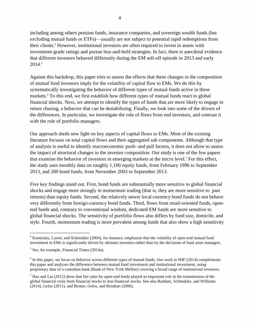
4

including among others pension funds, insurance companies, and sovereign wealth funds (but

excluding mutual funds or ETFs)—usually are not subject to potential rapid redemptions from

their clients.4 However, institutional investors are often required to invest in assets with

investment-grade ratings and pursue buy-and-hold strategies. In fact, there is anecdotal evidence

that different investors behaved differently during the EM sell-off episode in 2013 and early

2014.5

Against this backdrop, this paper tries to assess the effects that these changes in the composition

of mutual fund investors imply for the volatility of capital flow to EMs. We do this by

systematically investigating the behavior of different types of mutual funds active in these

markets.6 To this end, we first establish how different types of mutual funds react to global

financial shocks. Next, we attempt to identify the types of funds that are more likely to engage in

return chasing, a behavior that can be destabilizing. Finally, we look into some of the drivers of

the differences. In particular, we investigate the role of flows from end investors, and contrast it

with the role of portfolio managers.

Our approach sheds new light on key aspects of capital flows to EMs. Most of the existing

literature focuses on total capital flows and their aggregated sub components. Although that type

of analysis is useful to identify macroeconomic push- and pull factors, it does not allow to assess

the impact of structural changes in the investor composition. Our study is one of the few papers

that examine the behavior of investors in emerging markets at the micro level.7 For this effect,

the study uses monthly data on roughly 1,100 equity funds, from February 1996 to September

2013, and 200 bond funds, from November 2003 to September 2013.

Five key findings stand out. First, bond funds are substantially more sensitive to global financial

shocks and engage more strongly in momentum trading (that is, they are more sensitive to past

returns) than equity funds. Second, the relatively newer local-currency bond funds do not behave

very differently from foreign-currency bond funds. Third, flows from retail-oriented funds, open-

end funds and, contrary to conventional wisdom, dedicated EM funds are more sensitive to

global financial shocks. The sensitivity of portfolio flows also differs by fund size, domicile, and

style. Fourth, momentum trading is more prevalent among funds that also show a high sensitivity

4 Kaminsky, Lyons, and Schmukler (2004), for instance, emphasize that the volatility of open-end mutual fund

investment in EMs is significantly driven by ultimate investors rather than by the decisions of fund asset managers.

5 See, for example, Financial Times (2014a).

6 In this paper, we focus on behavior across different types of mutual funds. Our work in IMF (2014) complements

this paper and analyzes the difference between mutual fund investment and institutional investment, using

proprietary data of a custodian bank (Bank of New York Mellon) covering a broad range of institutional investors.

7 Hau and Lai (2012) show that fire sales by open-end funds played an important role in the transmission of the

global financial crisis from financial stocks to non-financial stocks. See also Raddatz, Schmukler, and Williams

(2014), Gelos (2011), and Broner, Gelos, and Reinhart (2006).

5

to global financial conditions. Finally, differences in volatility of flows from end investors play a

key role in explaining these patterns.8

Overall, these results suggest that the rising share of bond flows in recent years may have made

total portfolio flows to EMs more sensitive to global financial conditions, and more procyclical.

The rest of this paper is organized as follows. Section II describes the data and overviews fund

flows by their types. Section III describes the regression specifications and presents the results.

Section IV concludes.

II. OVERVIEW OF PORTFOLIO FLOWS FROM MUTUAL FUNDS

A. Data Description

Our mutual fund data source is EPFR Global, with a coverage of US$22 trillion in total assets as

of the end of 2013.9 The database covers a very large fraction of U.S. and European investment

funds, among others, and provides their basic characteristics such as investment styles,

domiciles, benchmarks, and geographic focus.10 We use EPFR Global’s monthly data with

information at the fund level, including on assets under management (AUM), inflows and

outflows (redemptions), and asset allocation by country. Based on this, we estimate the flow

from each fund to each country, adjusting for valuation effects.

The data cover a broad range of EMs and a relatively long time horizon. Our sample includes

current and former EMs since many countries currently considered advanced economies were

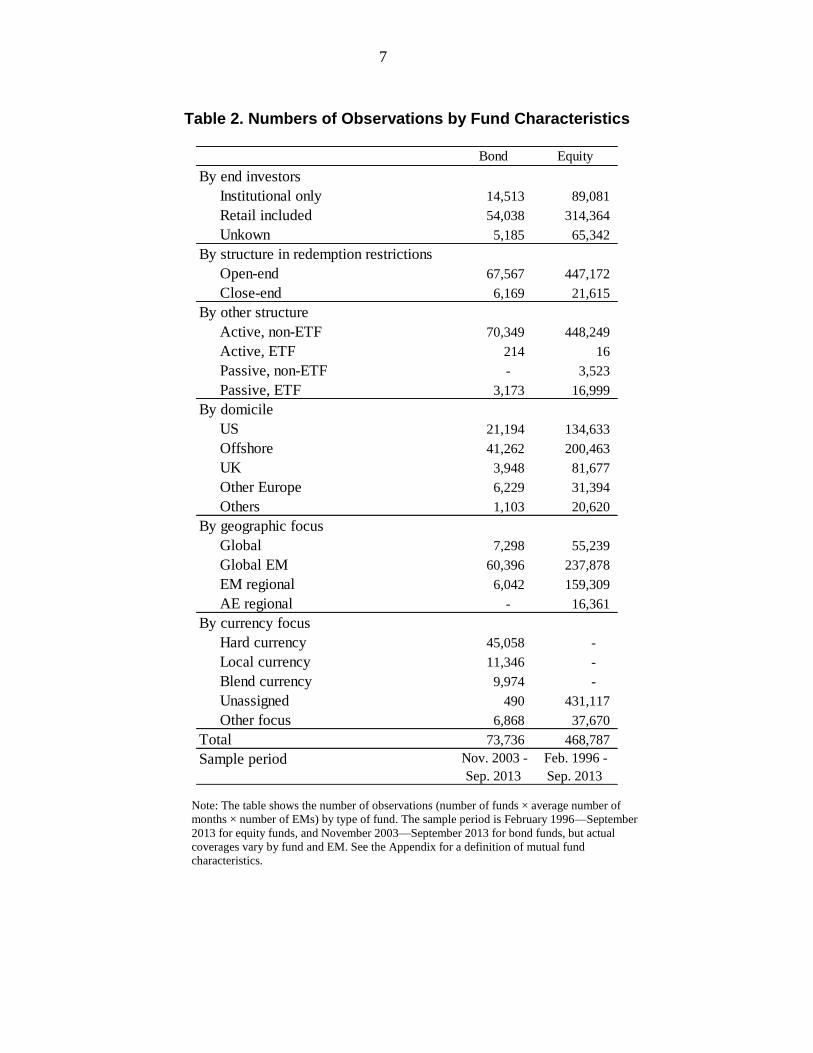
classified as EMs earlier in our sample period (Table 1).11 The data contain around 74,000 fund-

country-month observations from November 2003 to September 2013 for bond funds and around

470,000 observations from February 1996 to September 2013 for equity funds.12 Tables 2 and 3

show the distribution of the data by fund type and domicile.

8 This is particularly important to understand why crossover funds are less sensitive to global financial conditions

than EM-dedicated funds: crossover investors face less volatile flows from their ultimate investors, making their

capital flows more stable.

9 See Appendix for more details on the data and our procedures to obtain country flows from each fund, adjusting

for valuation effects.

10 See the Appendix for definition of mutual fund characteristics.

11 In addition, some advanced economies in IMF classification, mostly based on income levels, continued to be

classified as EMs in major asset indices. We exclude from the sample observations for offshore market economies,

economies that are extremely dependent on oil production, euro area countries often classified as EMs (e.g.,

Estonia), and economies without sufficient data.

12 The actual number of observations in our regression analysis changes in part due to the availability of explanatory

variables.

6

Table 1. Numbers of Observations by Investment Destination Economy

Note: The table shows the number of funds, the average number of months with data per fund, and the total number of

observations (number of funds × average number of months), country by country. The sample period is February 1996—

September 2013 for equity funds, and November 2003—September 2013 for bond funds, but actual coverages vary by fund.

Country

Number of

Funds

Average

Months by

Fund

Number of

Observations

Number of

Funds

Average

Months by

Fund

Number of

Observations

Argentina 96 39 3,737 327 36 11,739

Brazil 147 37 5,450 544 49 26,525

Bulgaria 46 24 1,109 24 16 392

Chile 84 25 2,130 395 40 15,730

China 103 20 2,096 726 47 34,102

Colombia 128 36 4,567 247 28 6,911

Croatia 63 18 1,135 98 22 2,196

Czech 3 27 81 330 40 13,230

Egypt 58 19 1,089 266 33 8,862

Hungary 107 23 2,463 340 49 16,746

India 78 11 850 627 46 28,831

Indonesia 144 33 4,701 576 46 26,575

Israel - - - 374 34 12,791

Latvia 28 7 209 10 17 172

Lithuania 50 24 1,217 6 27 160

Malaysia 140 26 3,708 533 48 25,842

Mexico 163 35 5,752 487 48 23,377

Nigeria 49 20 998 58 21 1,229

Pakistan 42 19 813 90 33 2,932

Peru 130 34 4,458 293 37 10,740

Philippines 91 40 3,621 454 37 16,678

Poland 128 26 3,377 370 45 16,645

Romania 45 11 501 59 20 1,208

Russia 144 34 4,889 544 45 24,514

Serbia 56 17 939 3 10 29

South Africa 136 27 3,634 479 40 18,944

Sout Korea - - - 674 53 35,657

Sri Lanka 51 20 1,003 60 42 2,547

Taiwan, P.C. - - - 634 53 33,763

Thailand 60 17 1,032 572 49 28,061

Turkey 133 33 4,413 417 46 19,280

Ukraine 83 34 2,804 107 15 1,649

Vietnam 39 25 960 31 24 730

Sample Period

Bond Funds Equity Funds

November 2003 - September 2013 February 1996 - September 2013

7

Table 2. Numbers of Observations by Fund Characteristics

Note: The table shows the number of observations (number of funds × average number of

months × number of EMs) by type of fund. The sample period is February 1996—September

2013 for equity funds, and November 2003—September 2013 for bond funds, but actual

coverages vary by fund and EM. See the Appendix for a definition of mutual fund

characteristics.

Bond Equity

By end investors

Institutional only 14,513 89,081

Retail included 54,038 314,364

Unkown 5,185 65,342

By structure in redemption restrictions

Open-end 67,567 447,172

Close-end 6,169 21,615

By other structure

Active, non-ETF 70,349 448,249

Active, ETF 214 16

Passive, non-ETF - 3,523

Passive, ETF 3,173 16,999

By domicile

US 21,194 134,633

Offshore 41,262 200,463

UK 3,948 81,677

Other Europe 6,229 31,394

Others 1,103 20,620

By geographic focus

Global 7,298 55,239

Global EM 60,396 237,878

EM regional 6,042 159,309

AE regional - 16,361

By currency focus

Hard currency 45,058 -

Local currency 11,346 -

Blend currency 9,974 -

Unassigned 490 431,117

Other focus 6,868 37,670

Total 73,736 468,787

Sample period Nov. 2003 -

Sep. 2013

Feb. 1996 -

Sep. 2013

8

Table 3. Numbers of Observations by Fund Domicile

Note: Number of fund-month observations (number of funds × average

number of months × number of EMs) by domicile of fund. The shadows

correspond to offshore market economies. “Other Europe” does not

include the United Kingdom and economies categorized in the offshore

market economies. “Other domiciles” includes Australia, Canada, Japan,

and the United Arab Emirates. The sample period is February 1996—

September 2013 for equity funds, and November 2003—September 2013

for bond funds, but actual coverages vary by fund and EM.

Bond Equity

Australia - 3,451

Austria 188 2,897

BVI - 2,350

Bahamas 464 -

Bahrain - 93

Belgium - 3,122

Bermuda - 2,566

Canada 1,007 16,754

Cayman 1,123 3,511

Denmark 5,786 5,433

Estonia - 455

Finland - 1,225

France - 11,673

Germany 255 2,722

Guernsey 3,309 10,584

Hong Kong - 297

Ireland 6,538 35,428

Japan 96 394

Jersey - 1,667

Lux 29,482 133,349

Mauritius - 294

NAntilles - 46

Netherlands - 1,306

Norway - 1,884

Singapore 346 1,137

Sweden - 677

Switzerland - 9,141

USA 21,194 134,633

Unassigned - 19

United Arab Emirates - 2

United Kingdom 3,948 81,677

Offshore 41,262 200,463

Other Europe 6,229 31,394

Other domicles 1,103 20,620

Total 73,736 468,787

Sample period Nov. 2003 -

Sep. 2013

Feb. 1996 -

Sep. 2013

9

B. Stylized Facts: Changes of Emerging Markets Portfolio Flow Structures

Since the early 2000s, bond flows have grown faster than equity flows. Between 2003 and 2013,

on average, annual bond flows to EMs amounted to 12.5 percent of AUM of mutual funds

included in the sample, compared to 5.1 percent for equity flows (Figure 1).

The relative importance of various types of mutual funds and their end investors also has

changed. Figure 2 shows that portfolio flows to EMs are increasingly intermediated through

open-end funds, passive ETFs, crossover funds, and local-currency bond funds. In particular:

The role of closed-end funds relative to that of open-end funds has declined. The growth

of (open-end) ETFs, which often are more fee- and tax effective than mutual funds for

end investors, is partly behind this trend.

The relative importance of passively managed funds (index funds, which track indices)

has grown. This again is closely related to the rapid growth of the ETF segment since

most of the ETFs are currently managed passively.13

The role of global funds (crossover funds) that invest both in EMs and DMs has grown

relative to dedicated EM regional funds. Moreover, among dedicated EM funds, global

EM funds (which invest in EMs around the world) have grown more rapidly than

regional EM funds.

Local-currency bond funds have expanded more rapidly than hard-currency bond funds.

This is partly the result of efforts by several EMs to overcome the “original sin” problem.

Mutual funds have been sold mainly to retail investors, but institutional investors have

been purchasing an increasing number of mutual fund shares. Some of this reflects the

expansion of defined contribution plans: in the United States, the percentage of defined

contribution plans’ assets in mutual funds has risen from 20 percent in 1993 to

60 percent in 2013 (ICI, 2014).14

Since 2009, flows to EMs from U.S. domiciled funds have grown relative to those from

offshore funds.

13 U.S. Securities and Exchange Commission allowed actively managed ETFs for the first time in 2008 (see

www.sec.gov/answers/etf).

14 This does not necessarily mean that there are more institutional investors active in the EM asset class as a whole. As IMF

(2011, 2014) observes, the size of the pension and insurance sectors has declined relative to mutual funds over the past two

decades. J.P. Morgan (2013) estimates that out of the EM fixed income securities held by global investors, about 40 percent is

held by global mutual funds, and about 60 percent is held by global institutional investors. There are some indications that the

share of mutual funds among global portfolio inflows to EM fixed income securities has increased over the past 10 years or so.

http://www.sec.gov/answers/etf

10

Figures 1–2 also show that not all types of fund flows are equally sensitive to global financial

shocks. For one, bond flows have been more volatile than equity flows. For instance, bond

outflows during the first six months after September 2008 (the collapse of Lehmann Brothers)

were 25.5 percent of total AUM, while equity outflows were only 5.1 percent. This pattern was

repeated in other episodes, including the one around mid-2013, when the Federal Reserve hinted

at the possibility of tapering its asset purchases. In addition, active funds (excluding ETFs),

open-end funds, EM regional funds, U.S. domiciled funds, and local currency bond funds seem

to be more sensitive to changes in global financial conditions, while passive ETFs, closed-end

funds, global or global EM funds, offshore funds, and hard currency bond funds are less sensitive

to these changes.

Finally, during some distress episodes, equity flows from institutional investors were more

resilient than those from retail investors.15 This is also true for bond funds during most crisis

episodes, except for the global financial crisis. These observations are in line with the notion that

institutional investors do not change their investment strategies frequently and are therefore less

sensitive to short-term market fluctuations.

Figure 1. Cumulative Bond and Equity Flows to Emerging Markets (1996–2013)

Sources: EPFR Global and authors’ calculations.

Note: The lines in the figure represent the log differences of the gross cumulative

flows of bond and equity funds to all EPFR-defined emerging markets economies

between period t and end 2010, multiplied by 100. EPFR estimates these aggregate

flows by taking the product of sample funds’ country allocation weights and end

investors’ flows to funds. Cumulative flows are calculated by chaining the flow-to-

assets under management ratio in order to adjust the effects from the expansion of

the database to cover more funds over time. For the same reason, we use cumulative

flows rather than assets under management to see the change of the relative size of

various mutual fund segments.

15 These episodes include the Asian crisis in 1997, the Russian crisis in 1998, the global financial crisis starting in 2007, the

European debt crisis in 2011, and the tapering episode in 2013.

-120

-100

-80

-60

-40

-20

0

20

40

60

Feb

-96

Feb

-97

Feb

-98

Feb

-99

Feb

-00

Feb

-01

Feb

-02

Feb

-03

Feb

-04

Feb

-05

Feb

-06

Feb

-07

Feb

-08

Feb

-09

Feb

-10

Feb

-11

Feb

-12

Feb

-13

Bond Equity

11

Figure 2. Cumulative Portfolio Flows to Emerging Markets by Fund Type: End Investors (1996–2013)

By redemption structures

By other structures

-140

-120

-100

-80

-60

-40

-20

0

20

40

60

No

v-0

3

No

v-0

4

No

v-0

5

No

v-0

6

No

v-0

7

No

v-0

8

No

v-0

9

No

v-1

0

No

v-1

1

No

v-1

2

Retail InstitutionalBond

-160

-140

-120

-100

-80

-60

-40

-20

0

20

40

Feb

-96

Feb

-97

Feb

-98

Feb

-99

Feb

-00

Feb

-01

Feb

-02

Feb

-03

Feb

-04

Feb

-05

Feb

-06

Feb

-07

Feb

-08

Feb

-09

Feb

-10

Feb

-11

Feb

-12

Feb

-13

Retail InstitutionalEquity

-120

-100

-80

-60

-40

-20

0

20

40

60

No

v-0

3

No

v-0

4

No

v-0

5

No

v-0

6

No

v-0

7

No

v-0

8

No

v-0

9

No

v-1

0

No

v-1

1

No

v-1

2

Closed-end Open-endBond

-100

-80

-60

-40

-20

0

20

40

60

Feb

-96

Feb

-97

Feb

-98

Feb

-99

Feb

-00

Feb

-01

Feb

-02

Feb

-03

Feb

-04

Feb

-05

Feb

-06

Feb

-07

Feb

-08

Feb

-09

Feb

-10

Feb

-11

Feb

-12

Feb

-13

Closed-end Open-endEquity

-200

-150

-100

-50

0

50

100

No

v-0

3

No

v-0

4

No

v-0

5

No

v-0

6

No

v-0

7

No

v-0

8

No

v-0

9

No

v-1

0

No

v-1

1

No

v-1

2

Active, non-ETF Passive, ETFBond

-500

-400

-300

-200

-100

0

100

Feb

-96

Feb

-97

Feb

-98

Feb

-99

Feb

-00

Feb

-01

Feb

-02

Feb

-03

Feb

-04

Feb

-05

Feb

-06

Feb

-07

Feb

-08

Feb

-09

Feb

-10

Feb

-11

Feb

-12

Feb

-13

Active, non-ETF Passive, ETFEquity

12

Figure 3. Cumulative Flows by Fund Type: Domicile (Cont.)

(1996–2013)

By geographic focus of investment

By currency focus

Sources: EPFR Global and authors’ calculations.

Note: The lines in the figure represent the log differences of the gross cumulative flows of bond and equity funds to all EPFR-

defined emerging markets economies between period t and end 2010, multiplied by 100. EPFR estimates these aggregate

flows by taking the product of sample funds’ country allocation weights and end investors’ flows to funds. Cumulative flows

are calculated by chaining the flow-to-assets under management ratio in order to adjust the effects from the expansion of the

database to cover more funds over time. For the same reason, we use cumulative flows rather than assets under management

to see the change of the relative size of various mutual fund segments. In our database, there are only a few actively managed

exchange traded funds and most of the passively managed funds are exchange traded funds, therefore, we bundle passively

managed funds and exchange traded funds together in the figure.

-120

-100

-80

-60

-40

-20

0

20

40

60

No

v-0

3

No

v-0

4

No

v-0

5

No

v-0

6

No

v-0

7

No

v-0

8

No

v-0

9

No

v-1

0

No

v-1

1

No

v-1

2

US OffshoreBond

-100

-80

-60

-40

-20

0

20

Feb

-96

Feb

-97

Feb

-98

Feb

-99

Feb

-00

Feb

-01

Feb

-02

Feb

-03

Feb

-04

Feb

-05

Feb

-06

Feb

-07

Feb

-08

Feb

-09

Feb

-10

Feb

-11

Feb

-12

Feb

-13

USA OffshoreEquity

-120

-100

-80

-60

-40

-20

0

20

40

60

No

v-0

3

No

v-0

4

No

v-0

5

No

v-0

6

No

v-0

7

No

v-0

8

No

v-0

9

No

v-1

0

No

v-1

1

No

v-1

2Global Global EM EM regionalBond

-100

-80

-60

-40

-20

0

20

40

Feb

-96

Feb

-97

Feb

-98

Feb

-99

Feb

-00

Feb

-01

Feb

-02

Feb

-03

Feb

-04

Feb

-05

Feb

-06

Feb

-07

Feb

-08

Feb

-09

Feb

-10

Feb

-11

Feb

-12

Feb

-13

Global Global EM EM regionalEquity

-250

-200

-150

-100

-50

0

50

100

No

v-0

3

No

v-0

4

No

v-0

5

No

v-0

6

No

v-0

7

No

v-0

8

No

v-0

9

No

v-1

0

No

v-1

1

No

v-1

2

Local Hard BlendBond

13

III. REGRESSIONS AND RESULTS

In this section, we examine more systematically the sensitivity of country flows to global

financial conditions and past returns, by estimating fund-level panel regressions. Since the

literature suggests that bond and equity flows behave differently, we run separate regressions for

bond and equity funds.16 In a second step, we focus on differences in sensitivities to global

shocks across different types of bond- and equity funds.

A. Behavior of Bond and Equity Funds

What, if any, are the differences in the drivers of flows between bond and equity funds? We

explore this question by estimating the following model with monthly data:

, , , 1 2 , , 1 3 , 4 , 1 , ,i j t i j t i j t j t j t i j tFlow Global Return ICRG RID , (1)

where Flowi,j,t is the ratio of the capital flow from fund i to country j to the AUM of fund i (see

Appendix). The first explanatory variable, Globalt, is a factor representing global financial

conditions. The expected sign of the coefficient 1 is negative because an increase in a global

factor (a deterioration of global financial conditions) is likely to result in more capital outflows.

Returni,j,t-1 is the lagged return of fund j in country i, and signals return chasing, which could lead

to more procyclical and volatile capital flows.17 To identify this effect more clearly, we separate

the impact of the global factor from that of lagged country returns by using the residual of a

regression of the latter on the global factor. ICRGj,t is the first difference of the ICRG

(International Credit Risk Guide) composite country risk rating and is a proxy for changes in

local macroeconomic conditions.18 Finally, RIDj,t-1 is the real interest rate differential relative to

the 1-month U.S. Eurodollar deposit rate and tries to capture search-for-yield by global investors.

The model also includes country-fund fixed effects i,j. A detailed description of the variables is

provided in the Appendix.

We estimate the model using several global factors. We first use the VIX (Chicago Board

Options Exchange Market Volatility Index), the implied volatility index for the S&P 500.

16 See Forbes et al. (2012), Fratzscher (2012), Raddatz and Schmukler (2012), and Puy (2013).

17 Typically, return chasing consists of buying past winners and selling past losers and is an apt description of the behavior of end

investors when selecting mutual funds (see, for instance, Zheng, 1999, Bollen and Busse, 2005, and Frazzini and Lamont, 2008).

We extend this concept to capital flows from mutual funds to EM asset returns. Return chasing of capital flows from mutual

funds could stem from both fund managers’ asset allocation decisions and end investor’s behavior to chase funds’ returns. In this

vein, Edelen and Warner (2001) show that aggregate mutual fund flows follow market returns in the U.S. equity markets; they

also find that high mutual fund investment flows into securities affect their prices and returns, possibly indicating positive

feedback effects between flows and asset prices.

18 Although unlikely, it is possible that mutual fund flows affect a country’s risk standing. In order to dispel endogeneity

concerns, we alternatively estimated (1) using lagged ratings. Our results are robust.

14

Although commonly used (see Forbes et al. 2012, Bruno and Shin, 2012, and Forbes and

Warnock, 2012), the VIX is an imperfect measure of global risk. For instance, the VIX remained

at a historically low level following the “tapering hint” of U.S. Fed in early 2013. Given these

shortcomings, as a robustness check, we use three other variables to capture different dimensions

of global risk: the TED spread, a measure of market liquidity; the Merrill Option Volatility

Expectations Index (MOVE), which captures uncertainty about future U.S. Treasury rates; and

the volatility of Eurodollar futures as a proxy for near-term uncertainty about U.S. monetary

policy (see also IMF 2014b). These global factors are positively correlated, but the correlations

are not all very large, and are not constant over time (Figure 4 and Table 4).

The results from the baseline estimation shown in Table 5 suggest that bond funds are much

more sensitive to global financial shocks and engage in “return chasing” more strongly than

equity funds. The coefficients on the VIX and the index return are statistically significant in all

regressions. However, the estimated coefficients of the regressions for bond funds are much

larger than those in the regression for equity funds (in absolute value), and the difference is

statistically significant. This result is robust when a common sample is used for the regressions

of equity and bond funds. The results are also robust to the use of alternative global factors

(Table 6). In addition, although not reported here, very similar results are obtained when adding

a measure of financial openness (Chinn and Ito 2006, Lane and Milesi-Ferretti 2007). In line

with our estimation results, the bond flows from mutual funds dropped more strongly than equity

flows during the market turbulence episode triggered by the uncertainty about U.S. monetary

policy in mid-2013 (Figure 1).

The estimated coefficients are economically significant. For instance, the estimates imply that an

increase in the VIX similar to that of the last four months of 2008—roughly 50 percent—leads

monthly bond flows to drop by 7.5 percent of AUM. This compares to average monthly bond

flows of one percent of AUM, between 2003 and 2013.

Given that the share of bond funds is rising, the estimation results imply that portfolio flows to

EMs are likely to become more sensitive to global financial shocks. This result has considerable

implications for capital flows as a whole for the following reasons. First, portfolio flows, as well

as banking flows, are more volatile than foreign direct investment and have played important

roles in the volatility of total capital flows. Second, the share of portfolio flows has risen while

that of banking flows has declined in recent years, partly because the deleveraging at European

banks. In fact, the surge of capital flows to EMs since the global financial crisis has largely been

led by portfolio bond flows.19

19

See IMF (2014a) for more detail.

15

Figure 4. Global Factors (1996–2013)

VIX TED spread

MOVE Volatility of Eurodollar Futures

Sources: Thomson Reuters Datastream and Federal Reserve Board.

Note: VIX is the Chicago Board Options Exchange Market Volatility Index. TED spread is the three-month

Eurodollar deposit rate minus the three-month U.S. Treasury bill rate. MOVE is the Merrill Option Volatility

Expectations Index.

Table 4. Correlation Coefficients across Global Factors (1996–2013)

Note: The correlation coefficients are computed using monthly

observations from February 1996 to September 2013. VIX is the

Chicago Board Options Exchange Market Volatility Index. TED is

the three-month Eurodollar deposit rate minus the three-month U.S.

Treasury bill rate. MOVE is the Merrill Option Volatility

Expectations Index.

0

10

20

30

40

50

60

70

Feb

-96

Jan

-97

Dec-

97

No

v-9

8

Oct

-99

Sep

-00

Au

g-0

1

Jul-

02

Jun

-03

May-0

4

Ap

r-05

Mar-

06

Feb

-07

Jan

-08

Dec-

08

No

v-0

9

Oct

-10

Sep

-11

Au

g-1

2

Jul-

13

(Percent)

0

0.5

1

1.5

2

2.5

3

3.5

4

4.5

5

Feb

-96

Jan

-97

Dec-

97

No

v-9

8

Oct

-99

Sep

-00

Au

g-0

1

Jul-

02

Jun

-03

May-0

4

Ap

r-05

Mar-

06

Feb

-07

Jan

-08

Dec-

08

No

v-0

9

Oct

-10

Sep

-11

Au

g-1

2

Jul-

13

(Percent)

0

50

100

150

200

250

Feb

-96

Jan

-97

Dec-

97

No

v-9

8

Oct

-99

Sep

-00

Au

g-0

1

Jul-

02

Jun

-03

May-0

4

Ap

r-05

Mar-

06

Feb

-07

Jan

-08

Dec-

08

No

v-0

9

Oct

-10

Sep

-11

Au

g-1

2

Jul-

13

(Basis points)

0.0

0.5

1.0

1.5

2.0

2.5

3.0

3.5Feb

-96

Jan

-97

Dec-

97

No

v-9

8

Oct

-99

Sep

-00

Au

g-0

1

Jul-

02

Jun

-03

May-0

4

Ap

r-05

Mar-

06

Feb

-07

Jan

-08

Dec-

08

No

v-0

9

Oct

-10

Sep

-11

Au

g-1

2

Jul-

13

(Percent)

VIX TED MOVE Eurodollar

VIX 1.00 0.53 0.67 0.36

TED 0.53 1.00 0.53 0.33

MOVE 0.67 0.53 1.00 0.77

Eurodollar 0.36 0.33 0.77 1.00

16

Table 5. Base Estimation Results: Sensitivity of Bond and Equity Flows vis-à-vis the Global Factor by Type of Funds

(VIX as a Global Factor)

Note: “Full” corresponds to the regressions using all available

observations (November 2003-September 2013 for bond

funds and March 1996-September 2013 for equity funds).

“Common” corresponds to the regression for equity funds

using the common coverage of countries and observation

period with bond funds. The p-values reported in brackets are

calculated using Driscoll and Kraay’s (1998) robust standard

errors. ***, **, and * indicate statistical significance at the 1,

5, and 10 percent levels, respectively. VIX is the Chicago

Board Options Exchange Market Volatility Index. Return is

the country index return. ICRG is the first difference of the

ICRG (International Credit Risk Guide) composite country

risk rating. RID is the real interest rate differential relative to

the 1-month U.S. Eurodollar deposit rate. See the Appendix

for more detail.

Bond

Full Full Common

VIX -0.150*** -0.048*** -0.052***

(0.000) (0.000) (0.001)

Return 0.037*** 0.008*** 0.008***

(0.004) (0.000) (0.000)

ICRG 0.515*** 0.248*** 0.288***

(0.002) (0.002) (0.003)

RID -0.015 0.007 0.014

(0.790) (0.649) (0.747)

Observations 73,089 453,420 280,038

R-squared 0.040 0.032 0.039

Equity

17

Table 6. Robustness Test: Sensitivity of Bond and Equity Flows vis-à-vis the Global Factor

(Alternative Global Factors)

Note: The p-values reported in brackets are calculated using Driscoll and Kraay’s (1998) robust standard errors. ***, **, and * indicate statistical significance at the 1, 5, and 10 percent levels, respectively. Global is the global

factor. TED spread is the three-month Eurodollar deposit rate minus the three-month U.S. Treasury bill rate.

MOVE is the Merrill Option Volatility Expectations Index. Return is the country index return. ICRG

(International Credit Risk Guide) is the first difference of the ICRG composite country risk rating. RID is the

real interest rate differential relative to the 1-month U.S. Eurodollar deposit rate. See the Appendix for more

detail.

B. Portfolio Flows and Other Fund Characteristics

Next, we investigate whether different types of funds respond differently to changes in global

factors by estimating a regression similar to (1), augmented by one fund characteristic at a

time:

, , , 1 2 , 1 3 , 1

4 , , 1 5 , 6 , 1 , ,

i j t i j t i t t i t

i j t j t j t i j t

Flow Global Chara Global Chara

Return ICRG RID

, (2)

where Charai,t-1 is a dummy variable that takes the value of one when fund i has a certain

characteristic of interest and zero otherwise. We use the interaction term of Charai,t-1 and

Globalt to examine the different sensitivities of portfolio flows to the global factor across

types of funds. If a certain type of fund has a higher sensitivity to global financial conditions

Bond Equity Bond Equity Bond Equity

Global -2.298*** -0.673*** -0.042*** -0.003 -1.549** 0.032

(0.000) (0.000) (0.000) (0.527) (0.011) (0.909)

Return 0.032** 0.008*** 0.034*** 0.009*** 0.038*** 0.009***

(0.018) (0.000) (0.001) (0.000) (0.000) (0.000)

ICRG 0.518*** 0.241*** 0.534*** 0.254*** 0.621*** 0.252***

(0.002) (0.003) (0.001) (0.002) (0.000) (0.002)

RID -0.087* 0.003 -0.029 0.005 -0.068 0.006

(0.088) (0.809) (0.605) (0.701) (0.214) (0.693)

Observations 73,089 453,420 73,089 453,420 73,089 453,420

R-squared 0.039 0.032 0.040 0.032 0.038 0.032

TED spread MOVE Volatility of Futures

18

than all other types of funds (reference group), we would expect the coefficient 2 to be

negative.20

A potential drawback of specification (2) is that it does not account for potentially correlated

fund characteristics. For instance, crossover funds tend to be larger than other funds and this

characteristic could merely reflect a size effect. Therefore, we also estimate a model

including multiple fund characteristic dummies simultaneously as follows:

, , , 1 2, , , 1 3, , , 1

4 , , 1 5 , 6 , 1 , ,

i j t i j t k k i t t k k i t

k k

i j t j t j t i j t


Return ICRG RID

. (3)

where Charak,i,t-1 is a dummy variable that takes one when fund i is of type k, and zero

otherwise. For equity funds in model (3), the reference group consists of funds that are

medium sized, sold to retail investors, open-end, actively managed, not ETFs, domiciled in

the United States, and with a global EM focus. For bond funds in model (3), the reference

group is further restricted to hard-currency bond funds. However, the geographic-focus and

currency-focus dummies are highly correlated, causing a multicollinearity problem.21 Thus,

we estimate two variations of the model (3) with multiple fund characteristic dummies for

bond funds; one without currency focus dummies, and another without geographic focus

dummies.

The analysis reveals interesting differences across types of funds. Table 7 reports the

estimated coefficients of the interaction term between the VIX and fund characteristics

(results for models (2) and (3) are in the “Single” and “Multiple” columns, respectively). A

negative sign indicates that flows from funds with certain characteristic in one type category

(for instance, global funds) but otherwise with the characteristics of the reference group

decline more than those from funds in the reference group when the VIX increases. Many

estimated coefficients are statistically and economically significant and the results are

generally robust to alternative global factors (see Appendix Tables 1, 2, and 3).22 We can

summarize the main findings as follows.

20 Since most fund-type dummies are time-invariant (such as being an open-end fund) the main effect of being a certain type

of fund (3) cannot be identified in fixed-effect models. We can identify the two effects separately only when the fund

characteristic varies over time (such as fund size).

21 This is because all EM regional funds and global EM funds generally report currency focus while global funds do not

report currency focus (therefore, their currency focus automatically becomes “others”).

22 For instance, the result of the single characteristic regression for global bond funds suggests that the sensitivity of global

funds and that of the other funds differ by 0.15, which is comparable to the absolute value of the sensitivity of bond flows

reported in Table 5.

19

Country flows from funds geared toward institutional investors tend to be less

sensitive to changes in global risk aversion than those from retail-oriented funds. This

is in line with the results reported in IMF (2014a) and consistent with institutional

investors focusing on long-term performance and retail investors being more fickle.

As expected, closed-end fund flows are less sensitive to changes in global risk factors

than open-end funds, as they are not subject to redemptions by end investors. Hence,

the decline of closed-end funds relative to open-end funds over the past two decades

has probably increased the sensitivity of EM capital flows to global financial

conditions.

For bond funds, flows from active non-ETFs are more sensitive to global financial

shocks than passive ETFs whereas for equity funds, there is no strong evidence that

flows from ETFs react more to global financial shocks than other types of funds.23

Therefore, we do not find strong support for the claim that recent rise of ETFs has

increased capital flow volatility or intensified EM sell-offs during 2013 and 2014 (see

Financial Times, 2014b).

Somewhat surprisingly, global funds are more stable sources of capital flows than

dedicated EM funds. This is contrary to the widely-held perception that crossover

funds are a more volatile source of funding for EMs, because their fund managers can

reallocate their portfolios completely away from EMs. This result holds even after

controlling for fund size. It is possible that the behavior of end investors – which

could differ for global and dedicated funds – is driving the result. This point is

examined in Subsection D.

Portfolio flows from local currency bond funds do not seem to be more sensitive to

global financial shocks than those of hard currency bond funds. In principle,

investment in newer products, such as local currency EM debt, should be more

sensitive to global factors than that in more seasoned products like hard currency EM

bonds. The fact that investment opportunities in local currency bond markets are still

limited to relatively more mature and larger EMs is a likely explanation for this

result.

Small bond and equity fund flows are more sensitive to the VIX, in line with the

notion that the presence of large investors can make smaller traders more aggressive

in their selling (Corsetti and others 2004).

Flows of funds domiciled in the United Kingdom and the United States are less

sensitive to changes in global factors than offshore funds and other European funds.

This may reflect the fact that the VIX, the measure of global risk used in these

regressions, is more closely related to economic conditions in the United Kingdom

23 Most non-ETFs are actively managed open-end funds, and non-ETFs constitute the majority of mutual funds.

20

and in the United States. In that case, EM assets may provide an important

diversification benefit for British and American investors.

Table 7. Estimation Results: Sensitivity of Bond and Equity Flows vis-à-vis the Global Factor by Type of Funds

Note: The table reports the estimated coefficients on the interactions between the VIX (the Chicago Board Options

Exchange Market Volatility Index) and fund characteristic dummies. “Single” corresponds to the estimate of each regression

with a single characteristic dummy, which is represented in (2). “Multiple” corresponds to the estimates of a regression with

multiple characteristic dummies, which is represented in (3). The reference group for model (3) consists of medium-sized

open-end funds (excluding exchange traded funds) sold to retail investors, actively managed, domiciled in the U.S., and

investing in emerging markets globally (in hard currency in case of bond). This is why the rows for these characteristics in

“multiple” columns are empty. ***, **, and * indicate statistical significance at the 1, 5, and 10 percent levels, respectively.

Inference is based on Driscoll and Kraay’s (1998) robust standard errors.

The main results listed above hold when we allow for differences across fund types in the

reaction to variables other than the global factor (Appendix Table 4). Model (4) includes

Single Multiple Multiple Single Multiple

By size

Small -0.078** -0.113* -0.105* -0.054** -0.031

Medium -0.001 -0.007

Large 0.058 -0.006 -0.005 0.046*** 0.031**

By end investors

Institutional only 0.021 0.054 0.062* 0.022** 0.005

Retail included -0.021 -0.022**


Open-end -0.181*** -0.042***

Close-end 0.181*** 0.044 0.067 0.042*** 0.019

By other structure

Active, non-ETF -0.172*** 0.011

Active, ETF -0.180 -0.252 -0.256

Passive, non-ETF -0.056 -0.102*

Passive, ETF 0.174*** 0.110 0.099 0.003 -0.041

By domicile

US 0.207*** 0.030**

Offshore -0.176*** -0.181*** -0.184*** -0.039*** -0.022

UK 0.210*** 0.209** 0.200** 0.042*** 0.047***

Other Europe -0.145*** -0.183*** -0.196*** -0.035 -0.029

Others 0.132* -0.061 -0.059 -0.019 -0.008

By geographic focus

Global 0.150*** 0.091** 0.023 -0.012

Global EM -0.033 0.042***

EM regional -0.100** -0.003 -0.060*** -0.045***

AE regional 0.017 -0.019

By currency focus

Hard currency -0.054

Local currency -0.014 -0.031

Blend currency 0.004 -0.068

Unassigned 0.010

Other focus 0.152*** 0.078*

Bond Equity

21

interaction terms between one fund characteristic dummy and all the other explanatory

variables.

, , , 1 2 , 1 3 , 1

4 , , 1 5 , 1 , , 1

6 , 7 , 1 ,

8 , 1 9 , 1 , 1 , ,

i j t i j t i t t i t

i j t i t i j t

j t i t j t

j t i t j t i j t


Return Chara Return

ICRG Chara ICRG

RID Chara RID

. (4)

The results are broadly comparable to those reported in Table 7.

C. Which Types of Funds Engage in Return Chasing?

Which funds have a stronger tendency to buy past winners and sell past losers? We use

model (4) to investigate this question. A positive coefficient for the interaction term between

the fund characteristic dummy and the country’s asset return would imply more return

chasing (momentum trading) by those funds.

The results are reported in Table 8. They show that return chasing is often prevalent among

funds that are relatively more sensitive to the VIX. For instance, return chasing is more

prevalent among open-end funds than among closed-end funds, as well as among EM

regional funds (compared to global or crossover funds). In addition, offshore funds and funds

from continental Europe engage more in momentum trading than U.K. funds.

There are, however, important exceptions, especially among bond funds. For example,

momentum trading seems to be more prevalent in bond funds with institutional investors’

money relative to retail funds. This result does not seem fully consistent with the result

reported in IMF (2014a), which shows that institutional investors do not engage in

momentum trading. The difference may lie in the source data for funds; the institutional

investors reported in EPFR Global’s mutual fund database are not necessarily the same as

those captured by the custodian data from Bank of New York Mellon (used in IMF, 2014a).24

24 The data are collected by the bank in its role as a custodian for many large institutional investors domiciled in many

jurisdictions throughout the world, which include pension funds, insurance companies, and some official reserve funds from

various countries, among others.

22

Table 8. Estimation Results: The Extent of Return Chasing by Fund Type

Note: The table reports the estimated coefficients on the interactions between fund characteristic

dummies and the lagged excess index return of the regression model (4). ***, **, and * indicate

statistical significance at the 1, 5, and 10 percent levels, respectively. Inference is based on

Driscoll and Kraay’s (1998) robust standard errors.

By size

Small -0.017* 0.003

Medium 0.010 0.004**

Large -0.002 -0.006***

By end investors

Institutional only 0.023** 0.000

Retail included -0.023** -0.000


Open-end 0.039*** 0.006***

Close-end -0.039*** -0.006***

By other structure

Active, non-ETF -0.046** -0.007

Active, ETF 0.235***

Passive, non-ETF 0.002

Passive, ETF 0.035* 0.009

By domicile

US -0.009 -0.001

Offshore 0.013* 0.004**

UK -0.005 -0.007***

Other Europe -0.008 0.008***

Others -0.034 -0.002

By geographic focus

Global -0.025** -0.009***

Global EM 0.009 -0.002

EM regional 0.012 0.005***

AE regional -0.002

By currency focus

Hard currency 0.024***

Local currency 0.006

Blend currency -0.028**

Unassigned -0.026**

Other focus -0.090

Bond Equity

23

D. Roles of End Investors and Fund Managers

Existing investments, their returns, and in- and outflows from mutual fund shareholders

determine the size of investible resources for any given fund. The managers of the fund

determine how to allocate those resources across assets, within the fund’s mandate. By

looking at fund-level country flow data, we can discern the direct influence of ultimate

investors and fund managers on the behavior of investment flows.

We apply the analysis of Raddatz and Schmukler (2012) to our data set. They essentially

decompose the flow from each fund to each country as:

, , , , , ,( )i j t i t i j t i tFlow Flow Flow Flow , (5)

where ,i tFlow is the flow from ultimate investors to fund i (expressed as a the ratio to the

total AUM of the fund). The first term of the equation corresponds to the contribution of

ultimate investors, while the second is the contribution of managers. If the manager always

allocates flows from ultimate investors to EMs to keep portfolio weights constant, Flowi,j,t =

Flowi,t holds and the flow to each country Flowi,j,t can be explained only with the first term.

On the other hand, if the manager changes allocation weights, the second term also plays a

role. Raddatz and Schmukler (2012) calculate the share of the total variance of flows that can

be attributed to each component for active, passive, equity, and bond funds. We calculate the

standard deviation of the ratio of the flow from ultimate investors to the total AUM and the

share of the total variance that is attributable to the flow from ultimate investors, for many

varieties of funds.25

The results confirm that differences in the stability of flows from ultimate investors are

behind the observed cross-fund heterogeneity of portfolio flows. In particular, funds that

have more stable ultimate investor flows are generally less sensitive to global financial

conditions and display a weaker tendency to engage in return chasing. For instance, when

compared to all other funds, global bond funds are less sensitive to global factors (the

estimated coefficient 2 in (2) is positive—0.150—and highly significant; see Table 7) and

past returns (the estimated coefficient 5 in (4) is negative—-0.025—and significant; see

Table 8). Global bond funds also have less volatile end-investor flows (a standard deviation

of 5 percent compared to over 7 percent for global EM funds and EM regional funds), and

have a smaller fraction of their variance explained by such flows (only 17.1 percent Table 9).

25 Our calculation differs from Raddatz and Schmukler’s (2012) in two technical aspects. First, they calculate the flow to

each country using the share of the country’s total assets represented by each fund, take the variance of each individual

component at the country level, and then average it across countries. We take the variance of each component at the fund-

country level and average it, as this is consistent with our fund-country-level regression analysis. Second, they divide the

flow by the AUM at the start of period, while we use the average of the AUMs at the start and end of period.

24

Table 9. Stability of End Investor Flows—Variance Decomposition

Note: “Standard deviation” is the standard deviation of the ratio of the flow from ultimate investors to a fund to the total

assets under management of the fund. “Share of variance” is the share of the total variance of the flows from funds to EMs

that can be attributed to the flows from ultimate investors. The share is obtained by taking the variance of components

corresponding to flows from ultimate investors and to allocation changes of fund managers at the country-fund level,

averaging it across country-fund pairs, and dividing the averaged variance corresponding to flows from ultimate investors by

the sum of the averaged variances (the covariance term is ignored). The standard deviations and variances are calculated

only for country-fund pairs for which at least five time-series data are available. Here, small (large) funds are defined as

funds that have been categorized as small (large) funds in more than a half of the available data.

Bond Equity Bond Equity

By size

Small 8.2 8.7 24.3 28.1

Medium 7.4 6.3 24.5 20.2

Large 4.9 3.5 20.2 13.0

By end investors

Institutional only 8.1 7.0 40.8 29.5

Retail included 7.0 5.7 20.3 17.3


Open-end 7.6 6.3 24.9 20.6

Close-end 1.3 2.8 6.4 6.0

By other structure

Active, non-ETF 7.1 6.1 21.0 18.5

Active, ETF 8.4 65.9

Passive, non-ETF 3.4 19.6

Passive, ETF 8.7 8.5 66.0 49.2

By domicile

US 5.1 4.9 22.4 17.2

Offshore 8.2 7.7 25.1 24.2

UK 6.4 5.3 21.8 15.3

Other Europe 7.0 6.5 20.7 24.0

Others 5.9 4.8 19.7 14.9

By geographic focus

Global 5.0 4.7 17.1 13.6

Global EM 7.5 6.6 24.6 21.3

EM regional 7.4 6.9 25.9 24.3

AE regional 4.6 11.5

By currency focus

Hard currency 8.2 26.4

Local currency 7.2 27.7

Blend currency 5.8 15.8

Unassigned 2.7 11.4

Other focus 5.1 17.5

Standard deviation (%) Share of variance (%)

25

IV. CONCLUSION

We have examined the behavior and determinants of mutual fund flows to emerging markets

in the last two decades, against the backdrop of substantial changes in the landscape of

portfolio investment in EM economies, both at the level of the global investor base and in

local financial markets. To shed light on the impact of some of these structural changes, we

have conducted a detailed examination of the behavior of different types of funds at the

microeconomic level. In particular, we have investigated how different types of funds react

to changes in global financial conditions, the extent to which they engage in return chasing,

and the relative importance of end investors in driving this behavior.

We find that the “maturing” of the EM asset class seems to have made capital flows more

volatile, more sensitive to global financial conditions, and more procyclical, despite much

more solid macroeconomic fundamentals in EMs. In particular, bond funds, which have

substantially gained in importance in the intermediation of funds to EMs, are relatively

sensitive to global factors, and engage relatively more in momentum trading.

However, we do not find support for the widely held view that the growth of crossover funds,

ETFs, and local currency bond funds are making EM portfolio flows more sensitive to global

financial conditions. In part, the lower sensitivity of crossover funds seems to be attributable

to lower fluctuations of flows from ultimate investors. Interestingly, funds also differ in their

behavior depending on their domicile: those located in the United Kingdom and in the United

States are less sensitive to changes in the VIX than funds domiciled elsewhere. These issues

warrant further research.

Overall, given the observed differences in behavior across funds, from a recipient’s country

perspective, knowing one’s investor base (including end investors) is important.

Understanding and diversifying the investor base, possibly by working closely with asset

managers, can help EM countries mitigate the volatility risk associated with international

capital flows while reaping the benefits from financial globalization.

26

APPENDIX I. EPFR GLOBAL MUTUAL FUND FLOWS DATA

EPFR Global covers about 11,000 equity funds and about 4,500 bond funds, with a combined

US$22 trillion in total assets as of the end of 2013. According to EPFR Global, its data track

more than 95 percent of EM-focused bond and equity funds. Most of them are mutual funds

and ETFs, though the database includes limited number of hedge funds. The share of U.S.

investment in EMs covered by EPFR Global is around 58 percent for equities, and more than

42 percent for bonds as of the end of 2012.26

The database covers primarily mutual funds, and does not cover all the investment fund

flows nor capital flows intermediated directly by institutional investors, and therefore it may

not provide the full picture of macro level portfolio flows. However, these coverage issues

are of little concern for our analysis. This is because we focus on differences across different

types of mutual funds to understand aggregate dynamics. Although funds not covered by

EPFR Global may tend to investors that can behave differently, it is unlikely that their

inclusion would affect our results.

EPFR Global’s high-frequency reporting (monthly for funds’ asset allocation by country as

well as daily and weekly data for selected indicators from sub-samples of funds) is also an

advantage compared to quarterly or annual data. Moreover, data recording methods of EPFR

Global are better suited for our purpose than the Balance of Payments (BoP) or Coordinated

Portfolio Investment Survey (CPIS). EPFR Global records transactions on nationality basis,

while the BoP and CPIS report on residency basis.27 The CPIS also misclassifies some bond

fund flows as equity flows (Felettigh and Monti, 2008).

A. Portfolio Flows to Each Country from Each Fund

Portfolio flows to each EM from each fund need to be calculated from asset allocation data,

adjusting for their change owing to the changes of portfolio assets’ value. For this, we

assume that the asset returns are well approximated by country index returns, following

Gelos and Wei (2005). The flow-to-AUM ratio of fund i for country j at month t is

calculated as:

, , , , , 1 , 1 ,

, ,

, , , , , 1 , 1

(1 )

( ) / 2

i j t i t i j t i t j t

i j t

i j t i t i j t i t

w A w A rFlow

w A w A

26 The U.S. investment is from the U.S. Treasury International Capital System. Here, EM economies are those listed in

Table 1.

27 For instance, if a corporate of an EM economy issues bonds through its London subsidiary, EPFR Global treats the bonds

as the liability of an entity in the EM economy, but the BoP and CPIS treat as the liability of a U.K. entity, which is

problematic to explain the behavior of the EM company. See Shin (2013) for this issue.

27

where wi,j,t is the allocation weight at the end of month t, Ai,t is the AUM at the end of month

t, and rj,t is the index return from t-1 to t. The estimated flow to a country from a fund in a

month is normalized by the average of the assets allocated to the country at the beginning and

end of the month. As indexes, we use the MSCI for equity funds, the GBI-EM for local

currency bond funds, and the EMBI Global for other bond funds. Since the GBI-EM is a

local currency index, we adjust its returns using bilateral exchange rates to obtain U.S.

dollars-denominated returns.28

B. Explanatory Variables

Global. The VIX is the implied volatility index for the S&P 500 as reported by the Chicago

Board Options Exchange. The TED spread is defined as the three-month Eurodollar deposit

rate minus the three-month Treasury bill rate. The MOVE is the average implied volatility

across a wide range of outstanding options on U.S. Treasuries. The volatility of Eurodollar

futures is the realized volatility calculated using daily changes in the Thomson Reuter’s

futures continuous series index of the 9th three-month futures in the corresponding month

and annualized by multiplying with the square root of 250. We use the end of month data for

the VIX, the TED spread, and the MOVE.

Return. The country index return is calculated as excess dollar returns of relevant indices

(namely, bond index for bond flows and equity index for equity flows) over one month U.S.

Eurodollar deposit rate. We use the MSCI for equity funds; the U.S. dollars-denominated

GBI-EM for local currency bond funds; and the EMBI Global for other bond funds. We use

one-month lagged return to mitigate the endogeneity concern. We also take three-month

moving averages since it is plausible that flows respond to the past returns with a lag of

several months (see, for instance, Jegadeesh and Titman, 1993). Since the individual country

index return is somewhat correlated with the global factor, we use its orthogonal component

relative to the VIX or the relevant global factor.

ICRG. The ICRG composite country risk rating is based on 22 variables, covering political,

financial, and economic risks. A higher rating means a lower risk.

RID. The one-month-lagged real interest rate differential calculated as the difference between

the local short term interest rate with a maturity of around one month and the U.S. short term

interest rate minus the difference in the one-year-ahead forecasts of CPI inflation from

Consensus Forecasts.

C. Definition of Mutual Fund Characteristics

We classify funds according to the following categories:

28 We apply some basic data clean up principles and discard samples when (1) there is a large (more than 0.1 percent)

internal inconsistency for AUM of a same fund at a same period in different parts of the database, possibly due to reporting

mistakes; and (2) computed fund flow per AUM is greater than 100% in absolute value.

28

Fund size. We define large and small funds as those above the 80th

and below 20th

percentiles of AUM in each month, respectively, labeling the remainder as medium

funds.

End investor type. Mutual funds have been sold mainly to retail investors, but

institutional investors have been purchasing an increasing number of mutual fund

shares, in part owing to the rise of defined contribution pension plans. EPFR Global

provides share-class data for each fund: some shares are targeted to retail investors

and the others are to institutional investors. Using these data, we identify whether a

fund is sold only to institutional investors or is sold also to retail investors. Many

funds do not report the types of ultimate investors for all of their shares. In such a

case, we indentify a fund as a retail fund when some of its shares are known to be

sold to retail investors. As a result, we limit the unidentified observations to around

7 percent of bond funds and around 14 percent of equity funds.

Open-end or closed-end. Investors can flexibly add to or redeem money from open-

end funds, but not with closed-end funds.

Investment style (active or passive) and ETF. Passive funds usually replicate a given

benchmark index. Fund managers of active funds exercise their judgment to over- or

underweight certain assets compared to their benchmarks. Most ETFs are passively

managed index funds while most non-ETFs (“mutual funds” in a narrow sense) are

actively managed. We use four combined characteristics: active, non-ETF; active,

ETF; passive, non-ETF; and passive ETF.

Fund domicile. Fund domicile roughly corresponds to the residence of ultimate

mutual fund shareholders, though the correspondence is not necessarily accurate,

especially for funds domiciled in offshore markets. We divide domiciles into five

regions: the United States; offshore market economies; the United Kingdom; other

European countries; and others. Table 3 reports the numbers of observations by

domicile. The table also indicates the definition of offshore market economies (see

IMF, 2008).

Geographic focus of the fund’s investment destination. We divide funds into four

groups: global funds; global EM funds; EM regional funds; and advanced economy

regional funds. For instance, global funds correspond to funds that are categorized as

“Global" or "Global ex-US" by EPFR Global.

Currency focus (for bond funds only). We use five groups: hard currency; local

currency; blend currency; unassigned; and other currency focus.

29

Table 1. Robustness Test: Sensitivity of Bond and Equity Flows vis-à-vis the Global Factor by Type of Funds

(Ted Spread as the Global Factor)

Note: The table reports the estimated coefficients on the interactions between the TED spread (the three-month Eurodollar

deposit rate minus the three-month U.S. Treasury bill rate) and fund characteristic dummies. “Single” corresponds to the

estimate of each regression with a single characteristic dummy, which is represented in (2). “Multiple” corresponds to the

estimates of a regression with multiple characteristic dummies, which is represented in (3). The reference group for model

(3) consists of medium-sized open-end funds (excluding exchange traded funds) sold to retail investors, actively managed,

domiciled in the U.S., and investing in emerging markets globally (in hard currency in case of bond). This is why the rows

for these characteristics in “multiple” columns are empty. ***, **, and * indicate statistical significance at the 1, 5, and 10

percent levels, respectively. Inference is based on Driscoll and Kraay’s (1998) robust standard errors.


By size

Small -1.234* -2.244*** -2.195*** -0.244 0.042

Medium -0.394 -0.142

Large 1.508** 0.507 0.748 0.351** 0.243

By end investors

Institutional only 0.763 1.265** 1.230** -0.125 -0.381*

Retail included -0.763 0.125


Open-end -3.293*** 0.259

Close-end 3.293*** 1.685*** 1.728*** -0.259 -0.526

By other structure

Active, non-ETF -3.600*** -0.727

Active, ETF -126.420* -135.289*** -134.144***

Passive, non-ETF -0.451 -0.881

Passive, ETF 3.666*** 3.920** 4.128** 1.285 0.909

By domicile

US 2.664*** 0.225

Offshore -2.224*** -1.983** -1.963* -0.365 0.000

UK 2.735*** 4.395*** 4.513*** 0.591*** 0.738***

Other Europe -2.211*** -2.044*** -1.990** -1.247*** -1.078***

Others 2.762*** 0.299 0.352 0.720 0.575

By geographic focus

Global 2.908*** 1.495** 0.526* 0.031

Global EM -0.905** 0.610***

EM regional -1.512** -1.085 -0.865*** -0.760***

AE regional -0.285 -0.704

By currency focus

Hard currency -1.376***

Local currency -1.233* -1.364

Blend currency 0.817* 0.358

Unassigned 0.838

Other focus 2.979*** 1.607**

Bond Equity

30


(MOVE Index as the Global Factor)

Note: The table reports the estimated coefficients on the interactions between the MOVE (the Merrill Option Volatility

Expectations Index) and fund characteristic dummies. “Single” corresponds to the estimate of each regression with a single

characteristic dummy, which is represented in (2). “Multiple” corresponds to the estimates of a regression with multiple

characteristic dummies, which is represented in (3). The reference group for model (3) consists of medium-sized open-end

funds (excluding exchange traded funds) sold to retail investors, actively managed, domiciled in the U.S., and investing in

emerging markets globally (in hard currency in case of bond). This is why the rows for these characteristics in “multiple”

columns are empty. ***, **, and * indicate statistical significance at the 1, 5, and 10 percent levels, respectively. Inference

is based on Driscoll and Kraay’s (1998) robust standard errors.


By size

Small -0.016 -0.021 -0.018 -0.022*** -0.017**

Medium -0.009 0.005*

Large 0.023** 0.007 0.006 0.008** 0.001

By end investors

Institutional only 0.014 0.032*** 0.035*** 0.013*** 0.006

Retail included -0.014 -0.013***


Open-end -0.056*** 0.002

Close-end 0.056*** 0.030* 0.036* -0.002 -0.008

By other structure

Active, non-ETF 0.032 -0.021*

Active, ETF -0.117 -0.144* -0.146*


Passive, ETF -0.027 -0.053 -0.051 0.032** 0.020

By domicile

US 0.051*** 0.007*

Offshore -0.045*** -0.044*** -0.042*** -0.008** -0.002

UK 0.028 0.024 0.022 0.009** 0.014***

Other Europe -0.024* -0.032** -0.033** -0.006 -0.001

Others 0.059*** 0.025 0.025 -0.010 -0.004

By geographic focus

Global 0.043*** 0.019** 0.002 -0.007

Global EM -0.017** 0.007***

EM regional -0.017 0.012 -0.010*** -0.009***


By currency focus

Hard currency -0.021*

Local currency -0.007 -0.004


Unassigned 0.028

Other focus 0.043*** 0.018

Bond Equity

31


(Volatility of Eurodollar Futures as the Global Factor)

Note: The table reports the estimated coefficients on the interactions between the volatility of Eurodollar futures and fund

characteristic dummies. “Single” corresponds to the estimate of each regression with a single characteristic dummy, which is

represented in (2). “Multiple” corresponds to the estimates of a regression with multiple characteristic dummies, which is

represented in (3). The reference group for model (3) consists of medium-sized open-end funds (excluding exchange traded

funds) sold to retail investors, actively managed, domiciled in the U.S., and investing in emerging markets globally (in hard

currency in case of bond). This is why the rows for these characteristics in “multiple” columns are empty. ***, **, and *

indicate statistical significance at the 1, 5, and 10 percent levels, respectively. Inference is based on Driscoll and Kraay’s

(1998) robust standard errors.


By size

Small -0.861 -0.881 -0.748 -1.134*** -1.046***

Medium -0.374 0.444**

Large 1.106* 0.380 0.215 0.220 -0.125

By end investors

Institutional only 0.853 1.718*** 1.700*** 0.652*** 0.258

Retail included -0.853 -0.652***


Open-end -2.433*** 0.413

Close-end 2.433*** 1.416 1.362 -0.413 -0.823**

By other structure

Active, non-ETF 0.844 -1.120

Active, ETF -6.228** -7.495*** -8.356***


Passive, ETF -0.465 -2.271 -2.417 1.442 0.973

By domicile

US 2.187*** 0.311

Offshore -1.485** -1.623** -1.824** -0.340 -0.045

UK 0.265 -0.453 -0.738 0.382 0.555*

Other Europe -2.054** -2.341** -2.241** -0.303 -0.164

Others 3.014*** 1.584 1.435 -0.413 -0.193

By geographic focus

Global 1.988** 0.811 0.075 -0.395

Global EM -0.796* 0.346

EM regional -0.862 0.126 -0.436 -0.456


By currency focus

Hard currency -1.691**

Local currency 1.069 1.722*


Unassigned 2.771

Other focus 1.984** 1.057

Bond Equity

32

Table 4. Robustness Test: Sensitivity of Bond and Equity Flows vis-à-vis the Global Factor by Type of Funds Using the VIX as the Global Factor and with

Interactions with Other Factors

Note: This table reports the estimated coefficients on the interactions between the VIX (the

Chicago Board Options Exchange Market Volatility Index) and one fund characteristic

dummy of the regression model (4), which includes additional interaction terms between the

fund characteristic dummy and variables other than the VIX. As in model (2), only one fund

characteristic dummy is included in the model at a time. ***, **, and * indicate statistical

significance at the 1, 5, and 10 percent levels, respectively. Inference is based on Driscoll

and Kraay’s (1998) robust standard errors.

By size

Small -0.085** -0.054**

Medium 0.003 -0.007

Large 0.055 0.047***

By end investors

Institutional only 0.009 0.021*

Retail included -0.009 -0.021*


Open-end -0.184*** -0.041**

Close-end 0.184*** 0.041**

By other structure

Active, non-ETF -0.154** 0.024

Active, ETF 0.705**

Passive, non-ETF -0.064

Passive, ETF 0.158*** -0.011

By domicile

US 0.213*** 0.028**

Offshore -0.182*** -0.038***

UK 0.218*** 0.043***

Other Europe -0.142*** -0.034

Others 0.087 -0.016

By geographic focus

Global 0.155*** 0.025

Global EM -0.035 0.043***

EM regional -0.102** -0.061***

AE regional 0.012

By currency focus

Hard currency -0.063*

Local currency -0.010

Blend currency 0.003

Unassigned 0.164***

Other focus -0.063

Bond Equity

33

REFERENCES

Bekaert, Greet, and Campbell Harvey, 2013, “Emerging Equity Markets in a Globalizing

World,” manuscript.

Bollen, Nicolas, and Jeffrey Busse, 2004, “Short-Term Persistence in Mutual Fund

Performance,” Review of Financial Studies, Vol. 18, No. 2.

Broner, Fernando A., Gaston Gelos, and Carmen M. Reinhart, 2006. “When in Peril,

Retrench: Testing the Portfolio Channel of Contagion,” Journal of International

Economics, Vol. 69, No. 1, pp. 203–30.

Chan-Lau, Jorge, and Li Lian Ong, 2005 “U.S. Mutual Fund Retail Investors in International

Equity Markets: Is the Tail Wagging the Dog?” International Economics and Finance

Journal, Vol. 1, No.1, pp. 73-88.

Chinn, Menzie D., and Hiro Ito, 2006, “What Matters for Financial Development?” Journal

of Development Economics, Vol. 81, No.1, pp. 163–92.

Corsetti, Giancarlo, Amil Dasgupta, Stephen Morris, and Hyun S. Shin, 2004, “Does One

Soros Make A Difference? A Theory of Currency Crises With Large and Small

Traders,” Review of Economic Studies, Vol. 71, No.1, pp. 87–114.

Driscoll, John C., and Aart C. Kraay, 1998, “Consistent Covariance Matrix Estimation with

Spatially Dependent Panel Data,” Review of Economics and Statistics Vol. 80, No. 4,

pp. 549–560.

Edelen, Roger, and Jerold Warner, 2001, “Aggregate Price Effects of Institutional Trading: A

Study of Mutual Fund Flow and Market Returns,” Journal of Financial Economics,

Vol. 59, Issue 2, pp. 195-200.

Felettigh, Alberto, and Paola Monti, 2008. ”How to Interpret the CPIS Data on the

Distribution of Foreign Portfolio Assets in the Presence of Sizeable Cross-border

Positions in Mutual Funds. Evidence for Italy and the Main Euro-area Countries,”

Questioni di Economia e Finanza (Occasional Papers) 16, Bank of Italy, Economic

Research and International Relations Area.

Financial Times, 2014a, “Investors Pull $12 bn from EM Stock Funds,” January 31.

______, 2014b, “EMs are Paying the Price of ETF Liquidity,” February 12.

Forbes, Kristin J., Marcel Fratzscher, Thomas Kostka, and Roland Straub, 2012, "Bubble

Thy Neighbor: Direct and Spillover Effects of Capital Controls," NBER Working

Paper, No.18052.

______, and Francis Warnock, 2012, “Capital Flow Waves: Surges, Stops, Flight and

Retrenchment,” Journal of International Economics, Vol. 88, No. 2, pp. 235-251.

34

Fratzscher, Marcel, 2012, “Capital Flows, Push Versus Pull Factors and the Global Financial

Crisis,” Journal of International Economics, Vol. 88, No. 2, pp. 341–56.

Frazzini, A, and Owen Lamont, 2008, “Dumb Money: Mutual Fund Flows and the Cross-

Section of Stock Returns,” Journal of Financial Economics, Vol. 88, Issue. 2, pp.

299-322.

Gelos, Gaston, 2011, “International Mutual Funds, Capital Flow Volatility, and Contagion–A

Survey,” IMF Working Paper, No.11/92.

_____, and Shang-Jin Wei, 2005, “Transparency and International Portfolio Holdings,”

Journal of Finance, Vol. 60, No. 6, pp. 2987–3020.

Hau, Harald, and Sandy Lai, 2012, “The Role of Equity Funds in Financial Crisis

Propagation,” unpublished manuscript, University of Geneva.

International Monetary Fund (IMF), 2008, “Offshore Financial Centers: Report on the

Assessment Program and Proposal for Integration with the Financial Sector

Assessment Program,” (Washington: International Monetary Fund).

_____, 2011, “Long-Term Investors and Their Asset Allocation: Where Are They Now?”

Chapter 2 of the September 2011 Global Financial Stability Report, (Washington:

International Monetary Fund).

_____, 2014a, “How Do Changes in the Investor base and Financial Deepening Affect

Emerging Market Economies?” Chapter 2 of the April 2014 Global Financial

Stability Report, (Washington: International Monetary Fund).

_____, 2014b, “Global Liquidity: Issues for Surveillance”, Policy Paper (Washington:

International Monetary Fund).

Investment Company Institute, ICI, 2014, 2014 Investment Company Fact Book.

Jegadeesh, Narasimhan, and Sheridan Titman, 1993, “Returns to Buying Winners and Selling

Losers: Implications for Stock Market Efficiency,” Journal of Finance, Vol. 48, No.

1, pp. 65-91.

Jotikasthira, Chotibhak, Christian Lundblad, and Tarun Ramadorai, 2012, “Asset Fire Sales

and Purchases and the International Transmission of Funding Shocks,” Journal of

Finance, Vol. 67, No. 6, pp. 2015–50.

J.P. Morgan, 2013, Where Are Emerging Markets Headed?, November.

Lane, Philip.R., and Gian Maria Milesi-Ferretti, 2006, “The External Wealth of Nations,

Mark II: Revised and Extended Estimates of Foreign Assets and Liabilities, 1970–

2004,” Journal of International Economics, Vol. 73, No.2, pp. 223–50.

35

Kaminsky, Graciela, Richard Lyons, and Sergio Schmukler, 2004, “Managers, Investors, and

Crises: Mutual Fund Strategies in Emerging Markets,” Journal of International

Economics, Vol. 64, No.1, pp. 113–134.

Puy, Damien, 2013, “Institutional Investors Flows and the Geography of Contagion,”

Economics Working Papers, ECO 2013/06, European University Institute.

Raddatz, Claudio, and Sergio Schmukler, 2012, “On the International Transmission of

Shocks: Micro-Evidence from Mutual Fund Portfolios,” Journal of International

Economics, Vol. 88, No. 2, pp. 357–74.

_____, Sergio Schmukler, and Tomás Williams, 2014, “International Asset Allocation and

Capital Flows: The Benchmark Effect,” Policy Research Working Paper 6866, World

Bank.

Shin, Hyun Song, 2013, “The Second Phase of Global Liquidity and Its Impact on Emerging

Economies,” Remarks at Federal Reserve Bank of San Francisco Asia Economic

Policy Conference.

Zheng, Lu, 1999, “Is Money Smart? A Study of Mutual Fund Investors’ Fund Selection

Ability,” The Journal of Finance, Vol. 54, Issue 3, pp. 901-933.

Date post:	27-Jul-2018
Category:	Documents
Upload:	doanhanh
View:	212 times
Download:	0 times

Changes in the Global Investor Base and the Stability of ... · Luis Brand. ão-Marques, Gaston...

Documents