WORKING PAPER SERIES

Changing Technology Trends, Transition Dynamics and Growth Accounting

Michael R. Pakko

Working Paper 2000-014F http://research.stlouisfed.org/wp/2000/2000-014.pdf

May 2000 Revised November 2005

FEDERAL RESERVE BANK OF ST. LOUIS Research Division 411 Locust Street

St. Louis, MO 63102 ______________________________________________________________________________________

The views expressed are those of the individual authors and do not necessarily reflect official positions of the Federal Reserve Bank of St. Louis, the Federal Reserve System, or the Board of Governors.

Federal Reserve Bank of St. Louis Working Papers are preliminary materials circulated to stimulate discussion and critical comment. References in publications to Federal Reserve Bank of St. Louis Working Papers (other than an acknowledgment that the writer has had access to unpublished material) should be cleared with the author or authors.

Photo courtesy of The Gateway Arch, St. Louis, MO. www.gatewayarch.com

Changing Technology Trends, Transition Dynamics and Growth Accounting

Michael R. Pakko*

Federal Reserve Bank of St. LouisP.O. Box 442

St. Louis, MO 63166

(314) 444-8564pakko@stls.frb.org

November 2005

Keywords: Capital deepening, productivity, transition dynamics

JEL Classification: E13, E22

Abstract

The technology growth trends that underlie recent productivity patternsare investigated in a framework that incorporates investment-specifictechnological progress. Structural-break tests and regime-shifting models revealthe presence of a downward shift in TFP growth in the late 1960s and an upwardshift in investment-specific technology growth in the mid-1980s. In both cases,these breaks precede the generally-recognized dates of labor productivity growthshifts. Simulations of technology growth shocks in a basic neoclassical modelshow that induced patterns of capital accumulation are generally consistent withthe observed lags between technological advances and changes in productivitygrowth.

* The views expressed in this paper are those of the author and do not necessarily reflect official positions of theFederal Reserve Bank of St. Louis, the Federal Reserve System or the Board of Governors.

1For example, Gordon (2000), Roberts (2001), and Jorgenson, Ho and Stiroh (2002) examine thetransitory and permanent components of productivity growth, with differing conclusions abouttheir relative contributions. However, these and other studies date the apparent change inproductivity growth at 1995 or 1996. Hansen (2001) finds a 1994 break in productivity growth.

2Solow (1987).

3The dating of the productivity growth slowdown in 1973 has become the received wisdom, fromat least as far back as Dennison (1985).

- 2 -

Changing Technology Trends, Transition Dynamics, and Growth Accounting

The increase in productivity growth since the mid-1990s has proven to bepersistent and durable. Having continued through a recession and into the currentexpansion, the acceleration of the late 1990s provides a counterpoint to the productivityslowdown of the early 1970s. Because the role of new technologies is commonly seenas central to the emergence of increased productivity growth, research on this growthresurgence has focused on advances in information-technology (IT), which is oftencharacterized as being “capital-embedded,” or “investment-specific” in its application.

A consensus has emerged that dates the increase in productivity growth in themid-1990s.1 However, the rapid pace of innovation in IT had been recognized longbefore that time. Indeed, the famous “Solow productivity paradox,” that we “see thecomputer age everywhere but in the productivity statistics” dates to nearly a decadeearlier.2

In this paper, I use a dynamic neoclassical growth framework to examine twoprominent, specific changes in technology growth trends of the past half-century, alongwith subsequent patterns of capital accumulation and productivity growth. Applying theapproach of Greenwood, Hercowitz and Krusell (2000) to measure Hicks-neutral andinvestment-specific technology as two independent sources of exogenous growth, theempirical evidence presented here suggests a negative structural break in neutraltechnology growth in the late 1960s and a partially offsetting positive break ininvestment-specific technology growth in the mid-1980s. In both cases, the estimatedbreakpoints precede the onset of shifts in labor productivity growth, as they have come tobe conventionally recognized.3

A number of explanations for a delayed impact of technological innovation onproductivity have been proposed in the literature. For example, some models incorporatelags associated with the adaptation and diffusion of technical knowledge (e.g. Hornsteinand Krusell, 1996; Jovanovic and MacDonald, 1994; Greenwood and Yorukoglu, 1997;Andolfatto and MacDonald, 1998; Yorukoglu, 1998; and Hornstein, 1999). Others

4In a previous paper on the subject of technology growth and transition dynamics (Pakko, 2002b),I examined a model that is subject to transitory shocks to both the level of technology and to thegrowth rate of technology—showing that the latter contribute significantly to the overall abilityof the model to explain the pattern of observed economic fluctuations.

- 3 -

Y K X Nt t t= −α α( )1

consider human capital accumulation as a specific source of the lag (e.g. Collard, 1999;Perli and Sakellaris, 1998; and Ozlu, 1996). Basu, Fernald and Shapiro (2001) proposeseveral sources of friction associated with adjustment costs and factor utilization rates. Models of “general purpose technologies,” as described in Helpman (1998), and otherR&D and Schumpeterian growth models like those of Aghion and Howitt (1992) alsosuggest delays in the productivity-enhancing effects of technological innovations. Historical analyses such as those of David (1990) and Mazzucato (2002) have been citedas evidence of some of these effects.

In this paper, I examine a more fundamental explanation involving the capital-deepening component of the standard neoclassical growth paradigm. Using dynamicsimulations of a model that accommodates stochastic trends in technological growthrates, I demonstrate how shifts in technology growth engender capital-stock transitiondynamics that tend to delay the response of productivity growth in a way that is generallyconsistent with patterns seen in the data.4

In particular, the model simulations are consistent with the evidence that theslowdown in neutral technology growth in the late 1960s was followed by a period ofincreased capital accumulation, delaying the evident onset of the productivity growthslowdown until the early 1970s; and that the acceleration of investment-specifictechnological progress in the 1980s was followed by a period of slow capital growth,suppressing labor productivity growth until the 1990s. The ability of this basic model togenerally match these features of the data suggests this endogenous capital-deepeningchannel as a potentially important factor in accounting for productivity growth patterns,in conjunction with the adaptation and diffusion lags that have been proposed in theliterature.

1. A Simple IllustrationBefore turning to an analysis of the data and the full articulation of the model, a

simple example can be used to illustrate growth-accounting implications of the capitaltransition dynamics considered in this paper. Consider a simple Cobb-Douglasproduction function with fixed labor supply and labor augmenting technical progress:

.

Along a steady state growth path, standard restrictions require the growth of output andcapital will be equal to the exogenous growth rate of technology: γY = γK =γX , where γ is

5As the coefficient of relative risk aversion approaches zero, the initial decline in capital growthbecomes smaller and the transition to the new steady-state growth path takes place more quickly. In the limit, with risk-neutral households, actual growth paths follow the technological potentialrates precisely. The transition paths in Figure 1 are generated by a model simulation usinglogarithmic preferences (σ =1).

- 4 -

∆ ∆ ∆ln ln( ) lnYN

ZKN

tt

t

= + ⋅

α (1)

used to denote (gross) growth rates. In the absence of investment-specific technologygrowth, consumption and investment grow at this common trend rate as well.

As a growth-accounting exercise, it is common to decompose labor productivitygrowth into components measuring TFP growth and capital-deepening:

where TFP growth, ∆ln(Zt)= (1-α)∆ln(Xt), is calculated as a residual. These twocomponents are often treated as being orthogonal, with the capital-deepening componentconsidered as a largely exogenous (or irrelevant) factor.

Now suppose that the steady-state growth rate of technological progress were toincrease from γX to γX=. The implied path of potential labor productivity growth and itscapital deepening component are illustrated by the solid lines in Figure 1.

In a setting where risk-averse households control the technology, makingintertemporal optimization decisions, the increase in the growth rate of technologicalprogress will be associated with an increase in equilibrium real rates of return: Using astandard isoelastic preference-specification, the long-run real interest rate depends on theconsumption growth rate, the coefficient of relative risk aversion, and the householddiscount factor, as given by the steady-state Euler equation: R = γc

σ/β.

At the higher rate of return implied by the increase in technology growth, theoptimal marginal product of capital rises, requiring the capital/labor ratio to fall. But theconsumption-smoothing behavior of households implies that capital growth will adjustonly incrementally to this new steady state path. Moreover, a wealth effect associatedwith the realization of a higher steady-state growth rate engenders an immediate increasein consumption, suppressing investment and capital accumulation so that capital growthinitially falls below its initial steady-state rate.5 Along the transition path, shown by thedashed lines in Figure 1, the capital-deepening component suppresses overall laborproductivity growth, so that it adjusts to its new steady-state growth path only graduallyover time.

[Figure 1]

6See, for example, Oliner and Sichel (1994, 2000, 2002); Jorgenson and Stiroh (1999); Jorgenson(2001); Stiroh (2002); and Jorgenson, Ho and Stiroh (2000,2002).

7As long as the production function is modeled as Cobb-Douglas, the specification in (2) isequivalent to the labor-augmenting form of technological progress discussed earlier:Yt=F[Kt,(XtNt)].

8Hercowitz (1998) relates this representation of investment-specific technological change to the“embodiment controversy”of Solow (1960) and Jorgenson (1966).

9For a more general discussion of the distinctions between these two sources of productivitygrowth, see Pakko (2002a).

- 5 -

Y Z K Nt t t t= −α α1 (2)

K K Q It t t t+ = − +1 1( ) .δ (3)

2. Neutral and Investment-Specific Technology Growth

The increase in productivity growth observed in the mid-1990s is commonlyattributed to advances in information-technology (IT). Consequently, research on thetopic has been particularly focused measuring the role of technological progress in thesesectors.6 An important feature of IT advances is that their effects are widely viewed asbeing embodied in the capital stock. Higher productivity arises from these advances notsimply because factors are utilized more efficiently, but because new forms of higher-quality capital have become available.

2.1 Theoretical Framework

One framework that represents this notion of embodiment is the investment-specific technology model proposed by Greenwood, Hercowitz and Krusell (1997,2000). The model includes the standard TFP form of technology:

where growth in Zt, is associated with balanced, or Hicks-neutral technological progress.7

Investment specific technological progress is represented in the capitalaccumulation equation:

Growth in the investment-specific technology index, Qt , is associated with progress thatis manifested through the accumulation of more efficient or higher quality capital goods.8 Output and productivity growth are affected indirectly as increases in Q raise theeffective capital stock that enters into the production function.9

10Components are aggregated using chain-weighting.

- 6 -

γ γ γK I Q= . (4)

γ γ γααα

Y Z Q= − −1

1 1 . (5)

The long-run growth rates of output and productivity depend on both technologyvariables, Zt and Qt, In conjunction with a budget constraint, we can derive the usualsteady-state restrictions that output, consumption and investment per capita will grow at acommon rate: γY = γC = γI. However, in the presence of investment-specific technologicalchange the growth rate of the capital stock also reflects improvements in the productiveefficiency of capital goods:

Working through the capital deepening channel, investment specific technologygrowth provides an independent source of growth for output and productivity. Specifically, the production technology determines the relationship between outputgrowth and the underlying technology growth rates as:

A shift in either the neutral or investment-specific technology growth rates gives rise to achange in the potential growth rate of output and productivity.

2.2 Measuring Investment Specific Technology

As emphasized by Greenwood, Hercowitz and Krusell (1997), growth accountingin the presence of investment-specific technological progress requires some modificationof the data from the national income and product accounts.

The model is denominated in consumption-units, with Qt representing the relativeprice of effective investment. Proper accounting for neutral and investment specifictechnology requires that the data reflect the same structure. Hence, real output andinvestment should be deflated from nominal quantities by using a consumption priceindex. Following the practice of previous analyses, the measure of consumption usedhere consists of nondurables plus services (less housing services).10 Output isrepresented by nominal gross domestic business product divided by the consumptionprice deflator. Output per hour is then calculated as the ratio of this measure ofproduction to total business sector hours from the BLS productivity accounts.

The measurement of quality change in the national accounts is an importantconsideration for constructing empirical counterparts to the model’s variables. In orderto provide an accounting that is complete as possible, previous studies have usedGordon’s (1990) estimates of quality-change that is not reflected in the official data.

The bottom line of Gordon’s study was that the official NIPA data (as constructedat the time) understated the true growth rate of spending for producers’ durableequipment by nearly 3 percentage points per year over his post-war sample period.

11For example, Greenwood, Hercowitz, and Krusell extended the Gordon data through 1990 byadding 1.5 percent to the growth rates of real investment spending for all categories exceptcomputers. Hornstein (1999) invoked a similar procedure to extend the estimate through 1997.

12Data are extrapolated using only the last ten years of the sample period in recognition Gordon’sobservation that the magnitude unmeasured quality change was generally much smaller in thelatter part of his sample period, “consistent with the straightforward hypothesis that the PPI doesa better job of correcting for quality change now than was true thirty-five or forty years ago.” (Gordon, 1990, p. 538).

13The data set was compiled prior to the BEA’s December 2003 revision of the data for fixed-assets.

- 7 -

Because Gordon’s data set extends only through 1983, previous estimates of investment-specific technology growth have been based on extrapolation of Gordon’s aggregatedata.11

But as BEA definitions and methodologies are updated and as relative shares ofthe components of equipment investment change over time, simple extrapolation ofGordon’s aggregate data becomes less satisfactory. Ideally, one would like to haveextended data series at the disaggregated level of Gordon’s original study. A lessambitious alternative is to extrapolate the drift ratios for each of Gordon’s 22 majorinvestment categories independently—accounting for changes in BEA definitions andmethodology—then aggregate the extrapolated data to calculate a new, extended series.

Such a procedure is implemented here, using estimates based on a linearextrapolation of Gordon’s drift ratios for the period 1973-83.12 The extrapolated driftratios were applied to the more recent NIPA price data to create extended quality-adjusted series for the individual categories of investment goods. The data for individualcategories were then chain-weighted to yield an aggregate quality-adjusted measure offixed investment in equipment and software.

Special attention was paid to changes in BEA definitions and methodology. Inparticular, adjustments were made to account for methodological changes that haveimproved the measurement of quality change, obviating the use of Gordon’s adjustmentfactors. One important innovation made in 1996 was the inclusion of software as aninvestment component. Gordon’s data set did not include software, so the official BEAmeasure for this component is used, assuming that quality-change is properly measured. Similarly, the BEA has devoted considerable effort to accurately measuring qualitychange for computers and peripheral equipment; hence, we assume that the bias found byGordon in the vintage data has been eliminated in contemporary time series estimates forthat component. Extrapolations of the data for communications equipment and autoswere also treated with special attention to take account of updated procedures adopted bythe BEA for measuring quality change in those categories. These and other details of thedata construction are documented in a Data Appendix.13

14 The BEA constructs measures of net stocks for individual components, then uses chain-weighted aggregation to build aggregates. The use of annual depreciation factors provides anapproximate adjustment for changes in the composition of the capital stock and total depreciationthat arise from this procedure.

15 In particular, the accumulation equation implies the steady-state relationship QI/K =[γK - (1-δ)]. Using a prime mark (‘) to indicate values from the unadjusted BEA data, the adjusted capitalstock is initialized from the relationship K/K ‘=QI [γK ‘- (1-δ)]/Q ‘ I ‘[γK - (1-δ)], where initialvalues were used for investment data, and the γK values were calculated using averages for thefirst ten years of output and Q-growth. This calculation, which relies on an assumption that thesample period began with the economy on (or close to) its steady-state growth path, yields initialvalues for the adjusted capital series of about one-third the level of the BEA data.

- 8 -

In addition to equipment and software, another important component of thecapital stock is nonresidential structures—accounting for approximately 35 percent ofnominal nonresidential fixed investment in the period 1948-2001. Gort, Greenwood, andRupert (1999) examined the measurement of quality improvement in structures, andestimated that the official NIPA investment data understate real, quality-adjusted growthby approximately 1 percent per year.

To account for this source of investment-specific technology growth, an adjustedmeasure of this component was constructed by adding 1 percentage point to each year’sgrowth rate in real nonresidential investment (subtracting 1 percent growth annually fromthe growth rate of its price index). The resulting adjusted series is then aggregated bychain-weighting with the adjusted measure of equipment and software investment, toproduce a quality-adjusted aggregate for total private nonresidential fixed investment.

1.3 Growth Accounting with Investment-Specific Technology

The data for quality-adjusted investment and its associated price index form thebasis for estimating the contribution of investment-specific technology to productivitygrowth. First an index of investment-specific technology, Q, is constructed as the ratioof the consumption price index to the price index for (quality-adjusted) investmentgoods.

The estimates of Q, along with associated data for quality-adjusted investment arethen used to construct an adjusted capital stock series that takes account of investment-specific technological progress. First, the NIPA data for investment and capital are usedto back out a series of implied depreciation factors, (1-δt).14 These factors are then usedto construct a capital-stock series using a perpetual-inventory method—that is, byreconstructing the capital stock using the capital accumulation equation (3) using thequality-adjusted investment data. The initial value for the capital stock is adjusted usinggrowth rate and level relationships implicit in the accumulation equation to relateinvestment/capital ratios in the adjusted and unadjusted BEA data.15 The growth rate of

16For both the growth-accounting exercise and the parameterized model simulations presentedbelow, capital’s share (α) is set to 0.30.

17 Hansen’s (2001) survey paper on techniques for identifying structural breakpoints includes adescription of each of the tests reported here.

- 9 -

the adjusted capital stock exceeds its unadjusted BEA counterpart by about 2.3 percentover the period 1950-2001, but the pattern of fluctuations in capital growth is affectedlittle by the incorporation of unmeasured quality improvement: the official and adjustedmeasures move closely together, having a correlation of 0.88. Regardless of the measureused, capital growth reached a peak in the late 1960s and slowed dramatically in the late-1980s.

With the capital stock adjusted to incorporate growth associated with investment-specific technological progress, the final step in the growth accounting procedure is tocalculate the remaining technology that takes the form of total factor productivity, usingthe growth accounting relationship in equation (1).16

Figure 2 shows the measures of technology derived from this procedure. Asfound in previous studies, the explicit inclusion of investment-specific technology growthhas the effect of lowering measured TFP growth. Since the early 1970s, growth in Zt hasbeen negligible on average, with potential productivity growth driven almost entirely byQt. Cursory inspection of the trends for the two types of technological progress alsosuggests the possibility that shifts in growth rates preceded changes in productivitygrowth in the early 1970s and mid-1990s: There is a clear slowdown in neutraltechnology growth in the late 1960s, and the appearance of an acceleration of investment-specific technology growth sometime in the mid-1980s.

[FIGURE 2]

3. Identifying Shifts in Technology Growth Trends

3.1 Tests for Structural Breaks

Formal time-series tests for structural breaks confirm the presence of these trendshifts. Modeling each of the technology growth series an AR(1) process with a constantterm, the tests reported in Table 1 present evidence of statistically significant breaks ineach of the technology series.17

For neutral technology growth, Bai’s (1994) least-squares variance test identifiesa clear breakpoint in 1967. Tests of structural change based on Chow sequences identifythe same date being associated with a shift in the constant term, as well as a shift in the

18Tests for structural breaks in an alternative measure of Q constructed using NIPA data–withoutadjustment for unmeasured quality-change–yield similar results, verifying that the estimatedbreakdate is

19Tests for a change in the autoregressive parameter alone (not reported in Table 1) suggest apossible break in 1989, but it is not statistically significant (p-value = 0.12).

20Cummins and Violante use a procedure similar the one used here, but they used time-seriesforecasting methods rather than simple linear extrapolation to extend the series. They did not,however, explicitly adjust for some of the methodological improvements adopted by the BEA thatare considered here. On average, the growth rate of investment-specific technology calculatedusing the Cummins and Violante data exceeds my measure by more than one percentage pointover the period 1984-2001.

- 10 -

full regression (a joint test for a break in the constant term and the autoregressivecoefficient). In both cases, supremum test statistics exceed Andrews (1993) criticalvalues for significance at the 5 percent level.

For investment-specific technology growth the specific timing of a structural shiftis not as clear, but its presence is nevertheless confirmed. The least-squares variance testidentifies 1983 as the breakdate, as does the Andrews test for a structural change in thefull regression.18 Testing specifically for a change in the constant term, there is a localmaximum in the Chow sequence in 1983 that exceeds a 10 percent Andrews test statistic,but it is dominated in the supremum test by a peak in 1987. The indication of a 1987breakdate for the mean is significant at the 10 percent level, with an approximate p-valueof 0.06 (calculated using the method of Hansen, 1997).19

Coefficient estimates from the regressions associated with these break dates indicate that the mean growth rate of neutral technology declined from 1.71 percent to0.13 percent in 1967, and that the growth rate of investment-specific technology rosefrom 2.22 percent to 3.70 percent in 1987. In terms of technologically feasible labor-productivity growth, equation (5) relates these estimates to an initial decline of 2.3percent, and a subsequent increase of 0.6 percent.

As a test of the robustness of these findings, Table 1 also reports break-point testsfor two alternative sets of technology growth rates. The first set uses the unadjusted BEAdata, the second uses the extrapolated values of Gordon’s drift-ratios for equipmentinvestment as estimated by Cummins and Violante (2002).20 The Cummins-Violantefactors were used to construct technology growth variables using an identical procedureto that described in the previous section.

- 11 -

TABLE 1:TESTS FOR STRUCTURAL BREAKS IN TECHNOLOGY GROWTH a

Least-Squares Chow Tests for Structural Breaks

Variance Testb Full Regression Constant Term

Variable Breakdate[90% C.I.]

Breakdate Sup(W) P-valuec Breakdate Sup(W) P-valuec

Z 1967 1967 12.808** .024 1967 8.454** .045

ZBEA 1967 1967 17.664** .003 1967 12.442** .007

ZCV 1967 1967 14.873** .010 1967 10.038** .021

Q 1983 1983 11.289** .047 1987 7.785* .061

QBEA 1983 1983 20.831** .007 1987 16.413** .001

QCV 1983 1983 31.316** .000 1983 13.691** .004

* (**) Exceeds the 90% (95%) critical values using a 20% trim, as calculated by Andrews (1993)a AR(1) specification of logged first differences; sample period 1951-2001.

b Breakdate and confidence interval estimation using the method of Bai (1994).c Approximate asymptotic p-values as calculated by Hansen (1997)

All three measures of neutral technology growth identify the 1967 breakpoint. Similarly, the least-squares variance tests and the Chow tests for a break in the fullregression suggest a shift in investment specific technology growth in 1983. Althoughtests of the series based on the Cummins-Violante data suggest a break in the constantterm in 1983 as well, the series using unadjusted BEA data confirms the 1987 breakpoint(at a higher significance level). That the unadjusted BEA data suggest the samebreakpoints as the adjusted data is reassuring—suggesting that the findings are notunduly biased by the extrapolation procedures used to update the Gordon data set.

As will be shown below, estimates from a Markov switching model also supportthe 1987 breakdate.

21French (2001) uses a similar approach for estimating changes in the trend of total factorproductivity growth.

- 12 -

[ ( )] [ ( )] ( )x s r x s st x xt x t xt xt xt− = − +− −µ µ σ ε1 1 (6)

prob s j s i p i jxt xt ij( | ) , , , .= = = =−1 1 2 (7)

ξξ ηξ ηt t

t t t

t t t|

|

|=

⊗

′−

−

1

1(8)

ξ ξt t t tP+ =1| | (9)

3.2 A Regime-Shifting Model

As an alternative approach to identifying shifts in technology growth rates, a two-state Markov-switching model (Hamilton, 1990, 1994) was fitted to each of thetechnology growth series.21 For xt =∆ln(Zt), ∆ln(Qt),

where the means, µ, and standard deviations, σ, are functions of the unobservable two-state index variable, sxt, and ~N(0,1). The indicator variables follow Markov chains:ε xt

In the estimation, state 1 is taken to be the initial state—the high-growth state for Z andthe lower-growth state for Q.

Hamilton’s (1994) method for estimating this type of model employs a Bayesianstate-space filtering algorithm for generating conditional estimates of the state at eachpoint in time. In particular, inferences about the state variable are estimated by iteratingon equations (8) and (9):

where the ξ are two-element vectors representing estimated probabilities of being instates 1 or 2, P is the Markov-transition matrix with elements given by (7), ηt is a vectorof the conditional densities, f(x | sxt ), and the symbol denotes element-by-element⊗multiplication.

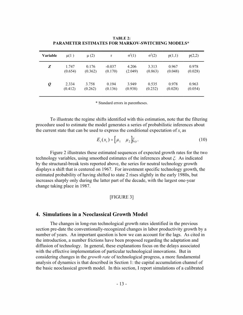
By assuming that the conditional densities are represented by mixed normaldistributions, equations (8) and (9) can be used to estimate the parameters of the modelvalues using maximum-likelihood techniques. The parameter estimates found using thisapproach are reported in Table 2. For both technology growth variables, the high-growthand low-growth states are quite persistent, with transition probabilities associated withstaying in the current state very close to one. Note that the mean growths rates are nearlyidentical to those found in the structural break-test regressions reported above.

- 13 -

[ ]E xt t t t( ) .|= µ µ ξ1 2 (10)

TABLE 2:PARAMETER ESTIMATES FOR MARKOV-SWITCHING MODELS*

Variable µ(1 ) µ (2) r σ2(1) σ2(2) p(1,1) p(2,2)

Z 1.747(0.654)

0.176(0.362)

-0.037 (0.170)

4.206(2.049)

3.313(0.863)

0.967(0.048)

0.978(0.028)

Q 2.334(0.412)

3.758 (0.262)

0.194(0.136)

3.949(0.938)

0.535(0.232)

0.978(0.028)

0.963(0.054)

* Standard errors in parentheses.

To illustrate the regime shifts identified with this estimation, note that the filteringprocedure used to estimate the model generates a series of probabilistic inferences aboutthe current state that can be used to express the conditional expectation of xt as

Figure 2 illustrates these estimated sequences of expected growth rates for the twotechnology variables, using smoothed estimates of the inferences about ξ. As indicatedby the structural-break tests reported above, the series for neutral technology growthdisplays a shift that is centered on 1967. For investment specific technology growth, theestimated probability of having shifted to state 2 rises slightly in the early 1980s, butincreases sharply only during the latter part of the decade, with the largest one-yearchange taking place in 1987.

[FIGURE 3]

4. Simulations in a Neoclassical Growth ModelThe changes in long-run technological growth rates identified in the previous

section pre-date the conventionally-recognized changes in labor productivity growth by anumber of years. An important question is how we can account for the lags. As cited inthe introduction, a number frictions have been proposed regarding the adaptation anddiffusion of technology. In general, these explanations focus on the delays associatedwith the effective implementation of particular technological innovations. But inconsidering changes in the growth rate of technological progress, a more fundamentalanalysis of dynamics is that described in Section 1: the capital accumulation channel ofthe basic neoclassical growth model. In this section, I report simulations of a calibrated

- 14 -

max ( , ),E U C Ntj

t j t jj

β + +=

∞

−∑ 10

C K K Q Z K Nt t t t t t t+ − − =+−[ ( ) ] / .1

11 δ α α (11)

[ ]β α δα αEU Q

U QQ Z K Nt

C t t

C t tt t t t

( ) /( ) /

( )⋅⋅

+ −

=+ +

+ + +−

+−1 1

1 1 11

11 1 1 (12)

DSGE model that trace out the endogenous capital-deepening effects of exogenouschanges in balanced and investment-specific technological growth rates.

Two versions of the model are considered: In the first – a “full information”specification – technology growth rates are subject to one-time shifts that areunanticipated, but fully recognized once they occur. This specification corresponds tothe stark nature of the structural break tests reported in Section 3.1. In the secondversion, agents are assumed to be solving the Markov-switching specification estimatedin Section 3.2. This version of the model can be thought of as representing a “Bayesianlearning” framework.

While the full information model is shown to provide a somewhat better overallfit to the data, the Bayesian learning version provides very similar long-run long runimplications, verifying the robustness of the model’s general implication that endogenouscapital-deepening is consistent with low-frequency patterns observed in the data.

4.1. Model Structure

The basic structure of the model is as follows: An infinitely-lived representativehousehold maximizes utility over consumption and leisure

subject to a budget constraint that incorporates both neutral and investment-specifictechnology,

Our interest here is to consider the effects of changes in the growth rates of Zt andQt on patterns of capital accumulation. The nature of these effects can beillustrated—and distinguished from those of transitory shocks to the level oftechnology—by considering the fundamental Euler equation governing capital stockdynamics:

An increase in the expected future level of either technology variable, Qt+1 or Zt+1,raises the expected future marginal product of capital. An increase in Qt also raises theeffective return to current investment. Shocks to the levels of the technology variables,whether transitory or permanent, have the effect of increasing investment demand,resulting in an increase in equilibrium investment and capital accumulation.

The effects of changes in the long-run growth rates of technology variables can beseen by examining a steady-state version of equation (10),

22Specifically, the solution algorithms of King, Plosser and Rebelo (1988a) are adapted to allowfor changes in underlying growth trend variables.

- 15 -

α δγ γβ

α σkN

C Q

+ −

=

−1

1( ) , (13)

kN

Z Q

=

− −

−

+ −−

−

γ γ β δα β

σα

α σα

α1

1 11

11

1( )

( ). (13')

where k = K/(γK)t, a stationary-inducing transformation (described more fully in thefollowing subsection).

Equation (13) states that the equilibrium net marginal product of capital is equalto the real rate of return in the economy, which in turn depends on the underlying growthtrends. (The parameter σ represents the coefficient of relative risk aversion inconsumption.)

Using the steady-state growth relationships (4) and (5), the capital/labor ratio can beexpressed directly as a function of the long-run technology growth rates,

It is straightforward to show that k/N is decreasing in γZ and γQ — a higher growthrate of technology, of either type, is associated with a lower capital/labor ratio. Anincrease in the growth rate of either technology variable has the direct effect of raisingthe growth rates of output, consumption, capital and productivity. However, therelationships shown in equations (13) and (13') reveal that the increase will also beassociated with a shift in the level of the capital stock (relative to labor) as the realinterest rate increases and the optimal marginal product of capital rises. By lowering theequilibrium capital/labor ratio, an increase in technology growth has a transitional effectof that dampens the growth rate of capital. The effects of a shift in technology growthare therefore quite distinct from those accompanying shocks to the level of technologyrelative to trend.

4.2 Simulation Methodology

Simulations of the dynamic responses to these shocks are generated using standardtechniques for solving a stationary log-linear approximation of the model, modified to allowfor long-run technology growth rates to be subject to occasional shifts.22

First, a stationary representation of the model is derived by dividing each of thetime-t variables by growth factors, Xit, where Xit+1 = γX Xit. As a result of thistransformation, these growth factors emerge as parameters of the stationary system. For

23The model also includes the standard equation that relates the marginal rate of substitutionbetween consumption and leisure to the marginal product of labor. The specific effects ofallowing for endogenous labor-leisure choice will be considered below.

- 16 -

γ δk t t t tk k q i+ = − +1 1( ) , (14)

[ ]βγγ

α δσ

α αEU c N q

U c N qq z k Nt

C t t t

C t t t

C

Qt t t t

( , ) /( , ) /

( ) .+ + +

+

−

+ + +−

+−−

−

+ −

=1 1 1

11 1 1

11

111

1 1 (15)

( )γγ δ

γδ

γ δk

kkt t

kt t tk k q i

− −

+ −

−− −

= ++( )

$ $ ( )( )

$ $ $ ,1

111

example, using lower case variables to represent transformed (stationary) variables [e.g.kt = Kt/Xkt], the capital accumulation becomes,

and the Euler equation takes the form

Equations (14) and (15) describe the important dynamics of the model economy,where changes in the lower case variables will now represent out-of-steady-statemovements.23 Equations (13) and (13') showed that the long-run effects of changes intechnology growth rates are reflected in the steady-state interest rate and the capital-laborratio. But equation (15) differs in that it includes dynamics associated with changes inthe marginal utility of consumption. Now, if we consider a shift in technology growththat changes the γ-terms in (15) the dynamic transition path will involve adjustment alongmargins on both the preferences-side and production-side of the model. As illustrated insection 1, risk-averse agents will seek to smooth consumption, which is associated with agradual adjustment of the capital-labor ratio. Moreover, a wealth causes consumptiongrowth to “jump” in the same direction as the change in technology growth, movingcapital growth (and the capital-deepening component of labor-productivity growth) in theopposite direction.

To simulate these transition dynamics, I use a standard method of taking log-linear approximations of the model’s equations around a baseline steady-state, thensolving the resulting dynamic system using methods like those described by King,Plosser and Rebelo (1988a) and King and Watson (1998). But rather than treating thegrowth-trend variables as fixed parameters of the system, they are allowed to be time-varying. For example, equation (14) is linearly approximated as,

where the carat or “hat” values represent proportional deviations of the variables fromtheir baseline steady-state values, and the time subscript on represents a change in$γ kt

24King and Rebelo (1993) employ a similar approach to simulating capital transition dynamics. Rather than considering changes in the technological growth rate, however, they evaluateperturbations of the capital stock from its long-run value to generate transition dynamics back tothe steady state. The two exercises are conceptually identical, tracing the transition path of thecapital stock from an initial out-of-steady-state position to its equilibrium steady-state value.

- 17 -

$ $ $ ; , .γ ρ γ εXt X Xt Xt X Z Q= + =−1 (16)

∆ k k kt k kt t t= + + − −γ γ$ $ $ .1

U C N C Nt t t t( , ) ln( ) ( ) / ( ),1 1 11− = + − −−χ ζζ (17)

the expected future growth rate relative to the baseline steady-state. Equations (4) and(5) relate the growth-rate variables in (14) and (15) to the underlying technology growthtrends, which are assumed to be exogenous variables of the system.

In general, the exogenous technological growth variables take the form,

In the full-information version of the model, the autoregressive parameters, ρX, are set tounity: breaks in the technology growth rates are immediately recognized and assumed tobe permanent. In the Bayesian learning version, those parameters will be determined bythe mapping of the Markov-switching processes onto the AR(1) structure of the linearlyapproximated system.

By treating the growth trends as exogenous and time-varying, the log-linearapproximation of the model is used to simulate approximate transition dynamics inresponse to a growth rate shifts.24 Simulated growth rates of the underlying variables canthen be recovered from simulations as the sum of the baseline steady-state growth rate,the change in the growth rate, and the first-differences of the simulated dynamicresponses of model variables; for example,

4.3 A Calibrated Demonstration

The model is calibrated at an annual frequency using long-run average data, andwith parameter values that are generally consistent with RBC analyses and growthaccounting exercises. Capital’s share of output, α, is set to 0.30, and the capitaldepreciation rate, δ, is calibrated to the average ratio of depreciation to the net stock ofnonresidential fixed private capital in the BEA’s Fixed Reproducible Tangible Wealthaccounts—approximately 6.5%. The household discount factor, β, is based on a realreturn to capital of 6%.

For the model simulations, the form of the utility function is specified as:

25The labor supply elasticity (with respect to the real wage rate) is given by ζ-1(1-N)/N, so that thecalibrated parameter values imply that this elasticity is approximately equal to one. This value ishigher than is typically found in microeconomic analysis, but lower than values commonly usedto calibrate macroeconomic models. The unitary elasticity is consistent with some recent workseeking to reconcile the discrepancy between the micro and macro literature; e.g., Chang and Kim(2003, 2005). In any case, the particular value of this parameter turns out to be quantitativelyunimportant in the analysis.

- 18 -

i.e., the coefficient of relative risk aversion is set to unity. The preference parameter χ isselected so that the fraction of time spent working of 0.24, and the labor supply elasticityparameter, ζ , is set to equal 3.25

To demonstrate the dynamic adjustment paths following changes technologygrowth and to compare the implications of neutral and investment-specific growthshocks, consider one-time shifts that permanently raise the trend rate of productivitygrowth by one-half percent, from 1.5% to 2.0%. For the purposes of this demonstration,investment-specific technology growth is calibrated to account for one-half of the initial1.5% growth trend. Changes in each of the two types of technology growth areconsidered independently, where each shift is calibrated to deliver the one-half percentchange in productivity growth, dln(γZt) = (1-α) ×.005 or dln(γQt) = [(1-α)/α] ×.005.

Figures 4 and 5 illustrate the transition dynamics associated with these shifts. Thegrowth rate of the capital stock, shown in Figure 4, illustrates the fundamentalendogenous dynamics of the long-run transition path. An increase in either type oftechnology growth raises the optimal marginal product of capital, giving rise to a periodof slower capital growth as the capital/labor ratio adjusts to its new level. As illustrated inFigure 1, the wealth effect on consumption demand creates an initial decline ininvestment, so there is a period during which capital growth falls below its initial trendrate before converging to the new higher rate. The slowdown is more pronounced for achange in investment-specific technology growth, reflecting the fact that this form worksdirectly through capital-deepening and is therefore associated with a larger eventualincrease in the growth rate of the capital stock.

[FIGURE 4]

Figure 5 shows the growth rates of labor productivity and its capital-deepeningcomponent, αK/N. These series display an additional source of dynamics that was notpresent in Figure 1: The initial wealth effect of the change in technology growth pertainsto leisure as well as consumption, so there is decline in the growth rate of labor supplyassociated with the recognition of the shock. The growth shifts are modeled as changesin expected future growth from period T forward, so that the potential productivitygrowth trend increases in periods T+1 and beyond. At time T, the wealth effect on labor

- 19 -

supply lowers work effort. Given the predetermined capital stock, this results in atransitory increase in the growth rates of both KT/NT and YT/NT. Thereafter, the transitionpath of the capital stock drives the adjustment dynamics of these growth rates.

[FIGURE 5]

Growth from capital deepening falls below its initial rate and only graduallyconverges to the new higher trend. As a result, labor productivity growth remains belowthe new long-run trend for some time. In the case of a shift in neutral technology growth,productivity growth reaches half of its ultimate increase only after 4 years. It takes 12years for productivity growth to reach 90 percent of its eventual increase. The effects oftransition dynamics following a shift in investment-specific growth are even moredramatic: Because it effects growth solely through the capital-deepening component, theinvestment-specific growth shift results in productivity growth falling below its originaltrend rate, and it takes 10 years before productivity growth reaches half of its long-runincrease; 90 percent of the adjustment is achieved only after 19 years have passed.

3.5 Model Simulations Using With Structural Breaks (Full Information)

This section presents simulations of the full-information model using values fortechnology growth rates and their shifts, as estimated in the structural-break testregressions.

Figure 6 compares the model’s predicted growth rates for labor productivity andthe capital labor ratio to those in the data. The model simulation identifies growth-ratepaths that appear to fit the longer-run trends in the data fairly well. The simulationproduces a surge in capital deepening in the late 1960s that has the effect of delaying theslowdown in productivity growth following the downward shift in neutral technologygrowth. In response to the increase in investment-specific technology growth in the late1980s, capital deepening and overall productivity growth slow before rising graduallytoward the end of the sample period. The correspondence between the simulations andthe data is clearest in the comparison of capital stock growth rates in the third panel ofFigure 6. Although the timing and magnitude of the turning points differ between actualand simulated series, both display a key peak in the late 1960s and a slowdown in the late1980s, followed by gradual adjustment to the new steady-state growth rates.

[FIGURE 6]

As shown in the first row of Table 3, the correlations between the simulated seriesand the data are 0.54 for productivity and 0.24 for the capital-deepening component. Note that these correlations do not simply reflect the effects of the exogenous shifts intechnology growth: The second row of Table 3 shows the correlation of actual data withthe steady-state growth components only, constructed by assuming that the relationships

- 20 -

in equations (4) and (5) hold period-by-period. Without the endogenous modeldynamics, the labor productivity correlation is slightly lower, but capital-deepeningcorrelation is essentially zero. A comparison of the slower-moving capital-stock growthrates shows this even more clearly: The correlation between actual and simulated growthrates is 0.48, while the correlation of the data with only the exogenous growthcomponents is negative. The positive correlation for capital and the capital deepeningcomponent of labor productivity are entirely attributable to the model’s endogenousdynamics.

TABLE 3: CORRELATIONS OF SIMULATED GROWTH RATES WITH DATA

FULL-INFORMATION MODEL

Annual Growth Rates Low-Pass Filtered Data*

Variable Y/N K/N K Y/N K/N K

Correlation of Actualwith Simulated Data 0.544 0.243 0.479 0.973 0.870 0.606

Correlation of Actualwith Growth

Component Only0.492 0.007 -0.295 0.864 -0.044 -0.411

* Filtered data are generated using the band-pass filter described by Christiano and Fitzgerald (2003), with a specification that isolates cyclical components with a periodicity of 12 years of longer.

Note that the higher-frequency variability in the labor productivity andcapital/labor ratio, attributable to the wealth effect on labor supply, does little tocontribute to the fit of the simulated variables to the data. Hence, the inclusion ofvariable labor-leisure choice would not appear to contribute to the ability of the model tomatch longer-run productivity growth patterns. In fact, these high frequency dynamicstend lower the correlations between actual and simulated series reported in Table 3.

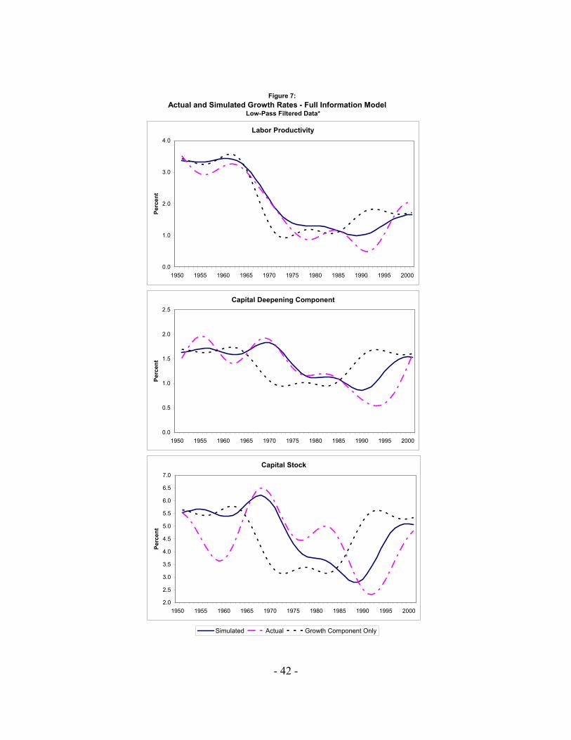
To focus more directly on the slower-moving components of fluctuations, Figure7 compares actual and simulated series that have been smoothed using the band-passfiltering method of Christiano and Fitzgerald (2003). A low-pass filter specification wasused to identify fluctuations in the data with cycle periodicity of 12 years or greater.

[FIGURE 7]

26This approach to constructing log-linear approximations of a Markov-switching process is asimilar to Schorfheide (2005), in which the long-run inflation rate is modeled as being subject toregime shifts. The analysis in this paper is a simplified application of the technique, which issupported by representation theorems in Sims (2001).

- 21 -

ln( ) ,γ µ µ=−

− −+

−− −

12

12

22

11 221

11

11 222

pp p

pp p (18)

The longer-run relationship between actual and simulated series is apparent in thesmoothed data, particularly for the capital growth rate and the capital-deepeningcomponent of productivity growth.. Though differing slightly in magnitude and phase,the low-frequency cycles isolated by the filter generally show striking similaritiesbetween actual and simulated series. Correlations comparing these series, also reportedin Table 3, show that the simulated and actual series are very highly correlated. Theexogenous growth shifts still account for much of the correlation between the filteredseries for labor productivity, but the model’s endogenous dynamics still fully account forthe correspondence between actual and simulated movements in capital growth and thecapital-deepening component of productivity growth. In the absence of endogenousdynamics, the correlations in the second line are both negative. The slight improvementin labor productivity correlations seen by comparing the two rows in Table 3 cantherefore also be attributed to the endogenous dynamics of the model.

3.6 Model Simulations with Regime-Shifting (Learning)

Perhaps a more realistic view of changes in technology growth rates is providedby the estimates from the Markov-switching model in Section 2.3. In this section, Iconsider simulations of a model in which agents are assumed to solve the inferenceproblem given by (6)-(9), allowing for “learning” about the shift in technology growthregimes.26

In order to map the regime-shifting framework onto the Canonical difference-equation structure of the model, we need to express a log-linearized version of theMarkov-switching process in the general form of equation (16).

It will be convenient to take the linear approximation around a baseline steady-state defined by the unconditional expectation of the two technology growth-rates,expressed as functions of the estimated parameters of the Markov-switching processes. For each of the technology growth variables, γ = γ Z, γQ ;

where the composite expressions weighting the mean growth rates are the ergodicprobabilities of being in the two states.

27See also Hamilton (1994), p. 684.

28That the autoregressive terms are close to, but not equal to one reflects the property of theregime-shifting model that there is always a small probability of moving to the other state.

29In this case, the initial conditions of the simulation are set by running the model for 30 yearsprior to the start of the sample, using the initial values of ξt|t (which are associated with a veryhigh probability of being in state 1 for both technology growth rates). This initialization period

- 22 -

( )$ ln( ) ln( )γ γ γ µ µ1 111

11 221 2

12

= − =−

− −−

pp p

( )$ ln( ) ln( )γ γ γ µ µ2 222

11 222 1

12

= − =−

− −−

pp p

[ ]$ $ $ |γ γ γ ξXt X X t t= 1 2 (19)

[ ]E Pt Xt X X t t( $ ) $ $ |γ γ γ ξ+ =1 1 2 (20)

ε γ γ γ ρ γXt Xt t Xt Xt X XtE= − = −− −$ ( $ ) $ $1 1 (21)

When γ is in state 1, its logarithmic deviation from the baseline steady-state is

and when γ is in state 2,

More generally, the conditional expectation of will depend on the estimated sequence$γ tof probabilities, ξt|t,

and from equation (9) the time-t expectation of xt+1 is

Note that the time varying nature of the growth states is entirely summarized inthe vector of probability inferences, ξ. For the two-state Markov processes considered, itcan be shown that is independent of the state, and is given by p11+ p22 - 1Et Xt Xt( $ ) / $γ γ+1(the stable eigenvalue of the probability transition matrix, P).27 For the linearlyapproximated simulations, this is the appropriate value to use for ρX in equation (16). Given the parameter values reported in Table 2, ρZ = 0.945 and ρQ = 0.941.28 Thesequence of disturbances fed into the model, which implicitly include terms associatedwith agents learning about the states, can then be calculated as:

The trend-shift estimates derived using smoothed inferences about the stateprobabilities, (illustrated in Figure 2) are used to generate a simulation of this version ofthe model.29 The results of this exercise, illustrated in Figure 8, show a somewhat muted

allows the capital stock to converge to near its steady-state value at the start of the sample period.

- 23 -

version of the simulated paths found in the full-information simulations of the model. The more gradual adjustment of expectations about changes in long-run growth ratesdampens the sharp response of labor that generated high-frequency movements in Y/Nand K/N in Figure 7, tending to improve the fit of the model. However, the learningframework also dampens the magnitude of capital-growth responses relative to the full-information simulations.

[FIGURE 8]

The correlations of actual and simulated data reported in Table 4 show that thelearning model provides a slightly improved fit for productivity and capital-deepeningrelative to the full information model, but with a slightly lower correlation between actualand simulated capital stock growth rates.

TABLE 4: CORRELATIONS OF SIMULATED GROWTH RATES WITH DATA,

REGIME-SHIFTING MODEL

Annual Growth Rates Low-Pass Filtered Data*

Variable Y/N K/N K Y/N K/N K

Correlation of Actualwith Simulated Data 0.553 0.369 0.405 0.967 0.828 0.476

Correlation of Actualwith Growth

Component Only0.515 0.010 -0.303 0.890 -0.002 -0.368

*Filtered data are generated using the band-pass filter described by Christiano and Fitzgerald (2003), with a specification that isolates cyclical components with a periodicity of 12 years of longer.

Again, to focus on the lower-frequency movements, Figure 9 shows actual andsimulated series that have been smoothed a low-pass filter. The longer-run movements inthe simulated series still correspond generally to patterns in the data, but fail to fit themagnitude of growth rate changes as well as in the full-information simulations. As wasthe case in the earlier simulations, however, the endogenous dynamics of the model areresponsible for the correspondence between actual and simulated growth rates of capital

- 24 -

and the capital-deepening component of productivity. In the absence of the model’sdynamics, the correlation of these growth rates with the underlying technology-growthshifts are zero or negative, in both the filtered and unfiltered data comparisons.

[FIGURE 9]

4. CONCLUSION

The model examined in this paper suggests that the adjustment of capital to achange in technology growth implies a long period of transition before the shift is fullyreflected in productivity growth. This is particularly true if the technology change isinvestment-specific.

Statistical tests show that there was, in fact, an increase in the rate of investment-specific technology growth in the late 1980s, partly reversing the decline in potentialgrowth from a downward shift in TFP growth in the late 1960s. The pattern of capitalstock growth and the capital-deepening component of productivity growth displaysubsequent fluctuations that are generally consistent with the model’s predictions. Thesefindings suggest that capital adjustment dynamics have been an important factorexplaining the apparent lag between the pace of technological innovation and the growthrate of labor productivity.

The adjustment mechanism identified in this paper contributes to an explanationof the lag, but is not proposed as an alternative to other theories that emphasizetechnology diffusion and adaptation. For explaining the lag between early advances inICT and their manifestation in aggregate measures of investment-specific technologygrowth, frictions associated with the adaptation and diffusion of technologicalinnovations are very likely relevant.

The fact that the model does not fully predict the timing or magnitude of the trough in capital-stock growth in the early 1990s suggests that the simple frameworksimulated in this paper fails to account completely for the lags between the identifiedshift in investment-specific technology growth and the productivity acceleration of thelate 1990s.

Nevertheless, the ability of the model to replicate some of the key salient featuresof the data suggests that the capital-adjustment channel examined here is important forevaluating patterns of productivity growth. The analysis suggests that the rapidproductivity growth of the late 1990s has its origins in accelerating technology trendsdating back nearly a decade, with the lag between the technology growth shift and theproductivity acceleration largely accounted for by the capital accumulation dynamics thatare implicit in a neoclassical growth paradigm.

APPENDIX

- 25 -

Data Appendix

A1. Basic Data Set: Summary

Variables are constructed as follows:

PI: A quality-adjusted measure of the price deflator for private nonresidential fixedinvestment. Details of the quality-adjustment methodology are described below.

PC: The price deflator for nondurable consumption goods and services, calculated as theratio of nominal expenditures on nondurables plus services to a chain weighted aggregateof those two consumption components (1996 dollars).

Q: The relative price of quality-adjusted investment goods in terms of consumption: PC /PI.

C: Real Consumption of nondurable goods and services, chain-weighted 1996 dollars.

I: Nominal private nonresidential fixed investment, deflated by PC.

Y: Nominal gross business output, deflated by PC.

K: The capital stock is generated iteratively from the accumulation equation, beginningwith a 1948 base of equipment and structures from the Fixed Reproducible TangibleWealth tables (BEA). Capital stock observations are updated using annual real figures forprivate nonresidential fixed investment and depreciation rates derived from the wealthtables (details below).

N: Hours of all persons, as used in the calculation of business sector productivity (BLS).

Z: The Solow residual, calculated using a capital share of 0.30 and a labor share of 0.70.

All variables are transformed into per capita terms using annual figures on total residentpopulation, as reported by the U.S. Census Bureau.

A2. Estimating and Incorporating Embodied Technological Change

In recent years, the BEA has been very diligent in adapting its methodologies tothe rapid rate of innovation in the information and communications technology (ICT)sectors. In addition to the introduction of hedonic indices for computer equipment andpurchased software, quality improvement has been examined and incorporated inmeasures for telephone switching equipment, cellular services and video players, amongothers. Indeed, the BEA has even changed its aggregation methodology to more

APPENDIX

- 26 -

accurately measure the contribution of quality change to GDP growth: the adoption in1996 of a chain-weighting methodology was intended to allow aggregates to trackquality-improvement better over time.

Nevertheless, many economists contend that a significant amount of qualitychange goes unmeasured in the official statistics, particularly in cases where qualityimprovement is more incremental. As detailed in his 1990 book, The Measurement ofDurable Goods Prices, Robert Gordon undertook to quantify the extent of thisunmeasured quality change. Drawing data from a variety of sources, including specialindustry studies, Consumer Reports, and the Sears catalogue, Gordon compiled a data setof more than 25,000 price observations. Using a number of methodologies, he compiledthe data into quality-adjusted price indexes for 105 different product categories, thenaggregated the data to correspond to the individual components of the BEA’s measure ofproducers durable equipment expenditure. In particular, he calculated a “drift ratio”,representing the difference between the growth rates of his quality-adjusted price dataand the official NIPA price indexes, then aggregated the components to create a new real,quality-adjusted investment series.

Table A1 shows trends in the drift ratios calculated by Gordon for individualcomponents of investment spending. The table is organized by the more recentcategories and definitions for Private Nonresidential Fixed Investment in Equipment andSoftware, which differs somewhat from the taxonomy used at the time of that Gordonconstructed his drift ratios. (Some specific differences will be discussed in more detailbelow). The growth rates in Table A1 represent the spreads between the official growthrates and the growth rates of Gordon’s quality-adjusted measures.

Over the span of the entire sample period, 1947-83, the drift ratios are uniformlypositive, indicating unmeasured quality improvement. In many cases, the magnitude ofthe quality adjustments is remarkable. Not surprisingly, Gordon’s estimates ofunmeasured quality improvement are particularly large for the high-tech categories ofcomputing and communications equipment (prior to the adoption by the BEA of hedonicmethodologies for these categories). Drift ratios for some components of transportationequipment, particularly aircraft, also indicate substantial under-measurement of qualitychange over the post-war period.

Generally speaking, the magnitude of the drift ratios is smaller in the later yearsof the sample period (and in some cases, marginally negative). This observation isconsistent with the hypothesis that the official statistics more accurately measure qualitychange in the 1970s and 1980s than they did in earlier decades.

The bottom-line of Gordon’s study was that the official NIPA data understatedthe true growth rate of investment spending by nearly three percentage points over hispost-war sample period. Unfortunately, because Gordon’s data set extends only through1983, some extrapolation is necessary in order to use his findings to evaluate recent U.S.economic experience.

APPENDIX

- 27 -

A3. Applying Gordon’s Adjustments to Recent Data

In order to apply Gordon’s quality adjustment to more recent NIPA data, it isnecessary to make some assumptions about unmeasured quality adjustment in the post-1983 period. In addition, changes in the BEA’s definitions and methodologyimplemented over the past two decades require some attention.

The basic procedure I adopt is to assume that the growth rate of unmeasuredtechnological change over the 1983-2001 period is the same as Gordon’s measured driftrate over the last 10 years of his sample. That is, Gordon’s actual drift ratios areextrapolated to 2001 using the growth rates in the second column of Table A1. The driftratios are renormalized to match the base period the NIPA data, then the price deflator foreach component is divided by the corresponding drift ratio to produce a quality-adjustedmeasure of price for each of the components of fixed investment. Deflating the nominalseries by these price indexes yield quality-adjusted measures of real investmentexpenditure.

The drift ratios are extrapolated on a component-by-component basis and thenaggregated to create a quality-adjusted measure of total investment spending. Thisdisaggregated approach is preferable to a simple extrapolation of the aggregate trend fortwo reasons: First, several changes in the BEA’s definitions and methodology have, forsome components, eliminated or at least mitigated the measurement problems found byGordon. In addition, the procedure of re-aggregating the quality-adjusted componentsusing a chain-weighting methodology allows the role of changing expenditure sharesover time to be incorporated into the total investment data.

Of the changes to the BEA’s definitions and methodology, most apply to theelements of information processing equipment and software. Many of these changes areconsistent with recommendations from Gordon’s study. First, the category previouslyknown as “office, computing and accounting machinery” (OCAM) was divided into twocategories: “computers and peripheral equipment” and “office and accountingequipment.” Most of the unmeasured quality change for this component was in thecomputers and peripherals element, for which a hedonic price index approach wasadopted in late 1985. Because current BEA practice carefully accounts for qualitychange, Gordon’s calculations are superfluous for evaluating the growth rate of computerequipment. For the remaining elements of that category, data from Gordon’s Tables 6.1and 6.2 (which detail the construction of a deflator for OCAM) were used to separate outthe computer component, with the remaining drift ratio to be applied to office andaccounting machinery.

Software was incorporated as a component of fixed investment only in 1999, andwas therefore not examined by Gordon. The BEA applies a hedonic approach to somecomponents of software investment: In particular, a hedonic index is used to deflateprepackaged software, while in-house software is deflated using an input cost index.

APPENDIX

30 See Parker (2000) and Landefeld and Fraumeni (2001).

31 Moulton and Seskin (1999).

32 Gordon, p. 538.

33 Fox (1987).

34 Fox and Parker (1991).

- 28 -

Custom software is deflated using a weighted-average of these two deflators.30 Thispractice amounts to applying a hedonic price index to about one-half of all software. Forthe purpose of this study, I assume that the BEA methodology accurately measuresquality change in software.

Next to computers, the largest drift ratios measured by Gordon were forcommunications equipment. In particular, Gordon found that the official price index fortelephone transmission and switching equipment (by far the largest item in thecommunications equipment category) vastly understated improvements associated withelectronics and transmissions technologies in the 1960s and 1970s. In 1997, the BEAintroduced a quality-adjusted price index for telephone switching and switchboardequipment, and carried back these revisions to 1985 in the 1999 comprehensive revisionof the national accounts.31 Because these revisions addressed the most serious concernsraised by Gordon about the measurement of quality change in communicationsequipment, I assume that the post-1985 data accurately reflect quality improvements. Consequently, I use Gordon’s drift ratios and extrapolations only for years prior to 1985.

Another category that requires special attention is automobiles. As shown inTable 3, the automobile component showed a negative drift ratio over the 1973-83period—suggesting that the BEA overestimated quality change over the decade. However, Gordon explains this finding as the result of a “spurious decline in the NIPAautomobile deflator during 1980-83”32 that he attributed to the use of a deflator for usedcars that is inconsistent with quality-change measured in the index for new cars. (Usedcar sold from business enterprises to households—reflecting a reclassification frombusiness capital to consumer durables—represent a factor that subtracts frominvestment.) In the absence of this inconsistency, Gordon notes that the drift ratio forautomobiles would be close to zero for the 1973-83 period. In 1987, the BEA began toadjust used automobile by applying a quality-adjustment factor derived from its treatmentof new car prices.33 In the comprehensive revision of 1991, this change was carried backto years prior to 1984.34 This change altered both the nominal and real data series oninvestment spending for automobiles, and largely eliminated the “spurious decline” in the

APPENDIX

35 In addition, because the BEA’s methodological changes affected both nominal and real series, Iuse Gordon’s actual price index figures (rather than applying his drift ratios directly to thecontemporary deflator series) for years prior to 1983.

36 This reclassification was associated with the incorporation of new data from the 1992 I-Oaccounts. See Taub and Parker (1997)

37 The “special industry machinery” component was one of six that Gordon referred to as“secondary” categories, for which the underlying price data overlapped with the other sixteen“primary” categories.

- 29 -

automobile deflator for 1980-83. Consequently, in extrapolating Gordon’s data onquality change for autos, I assume a drift ratio equal to zero for the post 1983 period.35

Some other re-classifications of the components of equipment investment provedto be simple to address: For example, the reclassification of analytical instruments fromthe Photocopy and Related Equipment category to the Instruments category in 199736

required no special adjustments, because Gordon’s drift ratio applies to the combinedInstruments and Photocopy Equipment category that was in use at the time. Similarly, areclassification of some equipment from Metalworking Machinery to Special IndustryMachinery was also innocuous, since Gordon found that the deflator for the latter wasbased on a subset of raw prices from the former. In calculating his drift ratios, Gordonsimply applied the same factor to both categories.37

Finally, there is the issue of aggregation methodology. At the time of his writing,Gordon criticized the BEA’s continuing practice of using fixed-weight deflators. Particularly in light of his modifications accounting for quality change, a fixed-weightapproach tends to underestimate the importance of goods that are declining in price (orincreasing in quality) while overstating the importance of goods that have rising prices. Gordon proposed the use of a Törnqvist index, which uses share weights from adjacentperiods to construct deflators for both the individual components of equipment purchases,and for aggregating the totals. The BEA subsequently adopted a “Fisher ideal” chain-weighting formula that is similar to the Törnqvist approach in that it incorporates share-weights from adjacent periods that are allowed to evolve over time. While the twoapproaches are very similar, they are not identical. For the purposes of this study,however, I assume that the two methodologies are essentially interchangable. While Iuse Gordon’s Törnqvist-aggregated measures disaggregating and re-aggregating theelements of OCAM into their contemporary definitional categories, I use the BEA’schain-weighting formula for aggregating the quality-adjusted components of investmentspending.

One further modification was made to the aggregate data on equipment andsoftware spending. Prices in 1974 and 1975 were distorted by the removal of wage-price

APPENDIX

38 See Katz and Herman (1997).

39 The net stocks calculated by the BEA are end-of-year values, with investment assumed to beplaced in service, on average, at mid-year. Consequently, it is assumed in the BEA data that new

- 30 -

K K It t t= − +−( )1 1δ (A1)

controls—a distortion that was exacerbated in Gordon’s data by the use of Searscatalogue prices from the spring-summer issue, which was printed before controls werelifted (see Gordon, p. 482). The growth rates of Gordon’s quality-adjusted pricestherefore exhibit large fluctuations 1974 and 1975. To prevent these extreme changesfrom having an undue influence structural-break tests, price level data for 1974 isadjusted by linearly interpolating between price levels of 1973 and 1975. Thismodification leaves the average of 1974 and 1975 growth rates unchanged, but eliminateslarge swings evident in the original data.

A4. Unmeasured Quality Change for Nonresidential Structures

The investment aggregate used in this paper includes both durable equipment andstructures. In order to account for unmeasured quality change in the structurescomponent of the aggregate, I use the estimate of Gort, Greenwood and Rupert (1999). That study finds that the quality-improvement in structures that is not captured in theofficial NIPA data amounts to approximately one percent growth per year. Consequently, I add one percentage point to each year’s growth rate in real nonresidentialstructures over the sample period, then construct an adjusted real series. This measure isthen aggregated by chain-weighting with the adjusted measure of fixed investment inequipment and software to produce a total quality-adjusted measure of privatenonresidential fixed investment.

A5. Construction of Capital Stock Data

With this measure of investment in hand, the final step in compiling a quality-adjusted data set is the construction of an aggregate capital stock measure. Theprocedure used to construct the capital stock measure involves modification of theBEA’s estimates of fixed reproducible wealth.38

The BEA uses a perpetual inventory method with geometric depreciation – thesame general form as in the capital accumulation equation in the model.

Each year’s capital stock is constructed as he sum of undepreciated capital from theprevious year plus gross investment.39

APPENDIX

assets depreciate during their first year in service at a rate equal to one-half of the annualdepreciation rate on existing assets. This minor deviation from the capital accumulation processassumed in the model was found to make very little difference in the pattern of adjusted capitalstock growth rates. Consequently, the simpler formula which includes no depreciation forcurrent-year investment goods was used.

40 The BEA constructs measures of net stocks for individual components, then uses chain-weighted aggregation to build aggregates. The use of these annual depreciation factorsapproximately adjusts for changes in the composition of the capital stock and total depreciationthat arise from this procedure.

- 31 -

qi k K/ ( ).= − −γ δ1 (A2)

kk

qiq i

ADJ

NIPAkADJ

NIPA NIPAkNIPA=− −

− −( )[ ( )]

( )[ ( )]γ δ

γ δ1

1(A3)

To parallel this construction, I begin be using equation (A1) with data for netstocks of private nonresidential capital and fixed investment to calculate a series ofimplied depreciation factors.40 Given a starting value for the capital stock, an adjustedmeasure is then constructed by applying these depreciation factors to the quality-adjustedinvestment series, corresponding to QtIt in the model. Because the capital stock variablein the model represents capital available for production in the current year, the data areshifted by one year so that end-of-year values for the capital stock in year T are dated torepresent beginning-of-period stocks in T+1.

The starting value for the capital stock is calibrated by exploiting the steady-stateproperties of the model. Specifically, the accumulation equation (3) in the paper impliesthat the investment/capital ratio depends on the capital stock growth trend and thedepreciation rate:

The ratio of the adjusted capital stock to the official BEA measure is therefore related tothe implied growth rates of the two measures, as well as the initial ratio of adjustedinvestment to NIPA investment:

The numerator incorporates quality-adjusted investment (qi) and the associated growthrate of capital, γK = γY γQ while the denominator is related to official investment (iNIPA)and a measure γQ calculated official NIPA price indexes. Taking 1948 to be the base year,the ratio of the quality-adjusted investment series to the official series is 0.44. Averagegrowth rates of output and the relative prices of investment to consumption over thesubsequent 10-year period (1948-58) imply ratio of kADJ to kNIPA that is approximatelyequal to 0.3.

- 32 -

Table A1:Drift in the Ratio of Official to Alternative Deflators for Components of

Private Nonresidential Fixed Investment in Equipment and Software Growth Rates (Percent)

1947-83 1973-83Information processing equipment and software Computers and peripheral equipmenta 15.33 7.37

Softwareb na naCommunication equipment 6.42 8.13Instrumentsc,d 3.50 2.99Photocopy and related equipmentc,d 3.50 2.99Office and accounting equipmente 6.80 6.82

Industrial equipmentFabricated metal products 1.78 -0.42Engines and turbines 3.50 0.47Metalworking machinery 1.15 0.96Special industry machinery, n.e.c.c 2.47 2.81General industrial, incl. materials handling, equipment 1.79 1.25Electrical transmiss., distrib., and industrial apparatus 2.09 0.40

Transportation equipmentTrucks, buses, and truck trailersc 3.00 0.56Autos 1.35 -2.07Aircraft 8.29 3.65Ships and boatsc 1.93 1.39Railroad equipment 1.47 1.78

Other equipmentFurniture and fixtures 1.44 0.53Tractors 1.41 3.17Agricultural machinery, except tractors 0.68 -0.19Construction machinery, except tractors 1.62 0.68Mining and oilfield machineryc 1.62 0.68Service industry machinery 3.15 3.64Electrical equipment, n.e.c. 1.08 0.18Otherc 1.98 1.68

SOURCE: Gordon (1990), Appendix B, Appendix C and Tables 6.11 and 6.12.

NOTES:a. The official BEA statistics now incorporate quality-adjustment using a hedonic-price index

approach, obviating the need to use Gordon’s figures.b. Software expenditures have been included in official measures only since 1999.c. Classified by Gordon as “secondary” category, with price data derived from primary categories.d. At the time of Gordon’s study, Instruments and Photocopy comprised a single component.e. Derived from data on the category of Office, Computing and Accounting Machinery, adjusted to

exclude computers and peripheralsn.e.c. = not elsewhere classified.

- 33 -

References

Andolfatto, David and Glenn M. MacDonald, “Technology Diffusion and AggregateDynamics,” Review of Economic Dynamics 1 (1998), 338-370.

Aghion, Phillipe, and Howitt. Peter, “A Model of Growth Through CreativeDestruction,” Econometrica 60, 323-51.

Andrews, Donald W. K. “Tests for Parameter Instability and Structural Change WithUnknown Change Point,”Econometrica, 61:4 (1993), pp. 821-856.

Bai, Jushan, “Least Squares Estimation of a Shift in Linear Processes.” Journal of TimeSeries Analysis 15:5 (1994), pp. 453-72.

Basu, Susanto, John G. Fernald, and Matthew G. Shapiro, “Productivity Growth in the1990s: Technology, Utilization, or Adjustment?” Carnegie RochesterConference Series on Public Policy 55 (December 2001), 117-65.

Chang, Yongsung, and Sun-Bin Kim, “From Individual to Aggregate Labor Supply: AQuantitative Analysis based on a Heterogeneous Agent Macroeconomy” WorkingPaper 03-5, Federal Reserve Bank of Richmond (2003).

__________ “On the Aggregate Labor Supply,” Federal Reserve Bank of Richmond,Economic Quarterly 91 (Winter 2005).

Christiano, Lawrence J. and Terry J. Fitzgerald, “The Band Pass Filter,” InternationalEconomic Review 44 (2003), 435-65.

Collard, Fabrice “Spectral and Persistence Properties of Cyclical Growth,” Journal ofEconomic Dynamics and Control 23 (1999) 463-488.

Cummins, Jason G., and Giovanni L. Violante, “Investment-Specific Technical Changein the United States (1947-2000): Measurement and Applications.” Review ofEconomic Dynamics 5 (2002), 243-84.

David, Paul A., "The Dynamo and the Computer: An Historical Perspective on theModern Productivity Paradox," American Economic Review Papers andProceedings (May 1990), 355-81.

Denison, Edward F., Trends in American Economic Growth, 1929-1982. WashingtonD.C., The Brookings Institution, 1985.

- 34 -

Fox, Douglas R., “The U.S. National Income and Product Accounts: Revised Estimates”Survey of Current Business 67 (July 1987), pp. 7-15.

__________, and Robert P. Parker, “The Comprehensive Revision of the U.S. NationalIncome and Product Accounts: A Review of Revisions and Major StatisticalChanges,” Survey of Current Business 71 (December 1991), pp. 24-40.

Fraumeni, Barbara M., “The Measurement of Depreciation in the U.S. National Incomeand Product Accounts.” Survey of Current Business 77 (July 1997), pp. 7-23.

French, Mark, W., “Estimating Change in Trend Growth of Total Factor Productivity: Kalman and H-P Filters Versus a Markov Switching Framework.” Board ofGovernors of the Federal Reserve System, Finance and Economics DiscussionSeries 2001-44, September 2001.

Gordon, Robert J., “Does the ‘New Economy’ Measure up to the Great Inventions of thePast?” The Journal of Economic Perspectives 14:4 (Fall 2000), 49-74.

__________, The Measurement of Durable Goods Prices, (University of Chicago Press,1990).

Gort, Michael, Jeremy Greenwood and Peter Rupert, “Measuring the Rate ofTechnological Progress in Structures,” Review of Economic Dynamics 2 (1999),207-30.

Greenwood, Jeremy, Zvi Hercowitz, and Per Krusell, “Long-Run Implications ofInvestment-Specific Technological Change,” The American Economic Review87:3 (June 1997), 342-62.

__________, “The Role of Investment-Specific Technological Change in the BusinessCycle,” European Economic Review 44 (January 2000), 91-115.

Greenwood, Jeremy and Mehmet Yorukoglu, “1974,” Carnegie-Rochester ConferenceSeries on Public Policy 46 (June 1997), 49-95.

Hamilton, James D., “Analysis of Time Series Subject to Changes in Regime,” Journal ofEconometrics 45 (1990), 39-70.

__________, Time Series Analysis (Princeton University Press, 1994).

Hansen, Bruce E., "Approximate Asymptotic P Values for Structural-Change Tests,"Journal of Business and Economic Statistics 15:1 (1997), 60-67.

- 35 -

__________, “The New Econometrics of Structural Change: Dating Breaks in U.S.Labor Productivity,” The Journal of Economic Perspectives 15:4 (2001), 117-128.

Helpman, Elhanan, ed. General Purpose Technologies and Economic Growth, MITPress, 1998.

Hercowitz, Zvi, “The ‘Embodiment’ Controversy: A Review Essay,” Journal ofMonetary Economics 41 (1998), 217-224.

Hornstein, Andreas, “Growth Accounting with Technological Revolutions,” FederalReserve Bank of Richmond, Economic Quarterly 85 (Summer 1999), 1-22.

__________, and Per Krusell, “Can Technology Improvements Cause ProductivitySlowdowns?” NBER Macroeconomics Annual 1996, 209-259

Jorgenson, Dale W., “The Embodiment Hypothesis,” Journal of Political Economy 74:1(February 1966), 1-17.

__________, “Information Technology and the U.S. Economy,” American EconomicReview 92 (March 2001), 1-32.

__________, Mun S. Ho, and Kevin J. Stiroh, “Projecting Productivity Growth: Lessonsfrom the U.S. Growth Resurgence,” Federal Reserve Bank of Atlanta EconomicReview 87:3 (2002:Q3), 1-13.

__________, and Kevin J. Stiroh, “Raising the Speed Limit: U.S. Economic Growth inthe Information Age,” Brookings Papers on Economic Activity 1(2000), 125-211..

Jovanovic, Boyan and Glenn M. MacDonald, “Competitive Diffusion,” Journal ofPolitical Economy 109 (February 1994), 24-52.

Katz, Arnold J., and Shelby W. Herman, "Improved Estimates of Fixed ReproducibleTangible Wealth, 1929-95," Survey of Current Business, May 1997, pp. 69-92.

King, Robert G., John Plosser and Sergio Rebelo, “Production, Growth and BusinessCycles: I. The Basic Neoclassical Model,” Journal of Monetary Economics21:2/3 (March/May 1988a), 195-232.

____________, “Production, Growth and Business Cycles: II. New Directions,” Journalof Monetary Economics 21:2/3 (March/May 1988b), 309-342.

- 36 -

King, Robert G., and Sergio Rebelo “Transitional Dynamics and Economic Growth in theNeoclassical Model,” American Economic Review 83:4 (September 1993), 908-31.

King, Robert G., and Mark W. Watson, “The Solution of Singular Linear DifferenceSystems Under Rational Expectations,” International Economic Review 39 (1998)1015-26.

Landefeld, J. Steven, and Barbara M. Fraumeni, “Measuring the New Economy.” Surveyof Current Business 81 (March 2001), pp. 23-40.

Landefeld, J. Steven, and Bruce T. Grimm, “A Note on the Impact of Hedonics andComputers on Real GDP,” Survey of Current Business 80 (December 2000), pp.17-22.

Landefeld, J. Steven, and Bruce T. Grimm, “Recognition of Business and GovernmentExpenditures for Software as Investment: Methodology and Quantitative Impacts,1959-98,” Manuscript, Bureau of Economic Analysis (2000). Available atwww.bea.doc.gov.

Landefeld, J. Steven, and Robert P. Parker, “BEA’s Chain Indexes, Time Series andMeasures of Long-Term Economic Growth,” Survey of Current Business 77 (May1997), pp. 58-68.

Mazzucato, Mariana, “The PC Industry: New Economy or Early Life-Cycle?” Review ofEconomic Dynamics 5:2 (April 2002), 318-345.

Moulton, Brent R., Robert P. Parker and Eugene P. Seskin, “A Preview of the 1999Comprehensive Revision of the National Income and Product Accounts: Definitional and Classificational Changes,” Survey of Current Business 79(August 1999), pp. 7-20.

Moulton, Brent R. and Eugene P. Seskin “A Preview of the 1999 ComprehensiveRevision of the National Income and Product Accounts: Statistical Changes,”Survey of Current Business 79 (October 1999), pp. 6-17.

Oliner, Stephen D. and Daniel E. Sichel, “Computers and Output Growth Revisited: HowBig is the Puzzle?” Brookings Papers on Economic Activity (1994), 273-317.

_________, “The Resurgence of Growth in the Late 1990s: Is Information Technologythe Story?” Journal of Economic Perspectives 14 (Fall 2000), 3-22.

__________, “Information Technology and Productivity: Where Are We Now andWhere Are We Going?” Federal Reserve Bank of Atlanta Economic Review 87(2002), 15-44.

- 37 -

Ozlu, Elvan “Aggregate Economic Fluctuations in Endogenous Growth Models,”Journal of Macroeconomics 18 (Winter 1996), 27-47.

Pakko, Michael R. “Investment-Specific Technology Growth: Concepts and RecentEstimates” Federal Reserve Bank of St. Louis Review (November/December2002a), 37-48.

__________, “What Happens When the Technology Growth Trend Changes? TransitionDynamics, Capital Growth and the ‘New Economy,’” Review of EconomicDynamics 5 (2002b), 376-407.

Perli, Roberto and Plutarchos Sakellaris, "Human Capital Formation and Business CyclePersistence," Journal of Monetary Economics 42 (1998), 67-92.

Roberts, John M., "Estimates of the Productivity Trend Using Time-Varying ParameterTechniques," Contributions to Macroeconomics 1:1 (2001), http://www.bepress.com/bejm/contributions/vol1/iss1/art3.

Schorfheide, Frank, “Learning and Monetary Policy Shifts,” Review of EconomicDynamics 8 (2005) 392-419.

Seskin, Eugene P., and Robert P. Parker, “A Guide to the NIPA’s” Survey of CurrentBusiness 78 (March 1998), pp. 26-68.

Taub, Leon W., and Robert P. Parker, “Preview of Revised NIPA Estimates for 1992From the 1992 I-O Accounts,” Survey of Current Business 77 (December 1997),pp. 11-15.

Sims, Christopher A., “Solving Linear Rational Expectations Models,” ComputationalEconomics 20 (2001), 1-20.

Solow, Robert M, “Investment and Technical Progress,” in Kenneth J. Arrow, SamuelKarlin, Patrick Suppes, eds., Mathematical Methods in the Social Sciences. Stanford University Press, Stanford CA, 1960.

__________, “Manufacturing Matters,” New York Times Book Review (July 12, 1987),36.

Stiroh, Kevin J., “Information Technology and the U.S. Productivity Revival: What Dothe Industry Data Say?,” American Economic Review 93 (2002), 1559-76.

Yorokoglu, Mehmet, “The Information Technology Productivity Paradox,” Review ofEconomic Dynamics, 1:2 (1998), 551-592.

- 38 -

Figure 2: Neutral and Investment-Specific Technology

(Log levels, Base = 1950)

Neutral Technology

0.0

0.1

0.2

0.3

1950 1955 1960 1965 1970 1975 1980 1985 1990 1995 2000

Investment-Specific Technology

0.0

0.3

0.6

0.9

1.2

1.5

1950 1955 1960 1965 1970 1975 1980 1985 1990 1995 2000

- 39 -

Figure 3:Growth Rate Estimates from a Markov-Switching Specification

0.0

0.5

1.0

1.5

2.0

2.5

3.0

3.5

4.0

1950 1955 1960 1965 1970 1975 1980 1985 1990 1995 2000

Gro

wth

Rat

e (P

erce

nt)

Investment-Specific Technology

Neutral Technology

Figure 4:Capital Stock Responses to Technology Growth Shifts

2.0

2.5

3.0

3.5

4.0

4.5

5.0

-5 0 5 10 15 20 25

Years from shift (T+j)

Gro

wth

Rat

e (P

erce

nt)

2

2.5

3

3.5

4

4.5

5

Investment-Specific

Neutral

- 40 -

Figure 5:Growth Accounting WIth Shifts In Technological Progress

A Neutral Technology Growth Shift

0.0

0.5

1.0

1.5

2.0

2.5

-5 0 5 10 15 20 25

Years from Shift (T+j)

Gro

wth

Rat

es (P

erce

nt)

An Investment-Specific Technology Growth Shift

0.0

0.5

1.0

1.5

2.0

2.5

-5 0 5 10 15 20 25

Years from Shift (T+j)

Gro

wth

Rat

es (P

erce

nt)

Labor Productivity

Capital Deepening

Capital Deepening

Labor Productivity

Implied Potential

Implied Potential

- 41 -

Figure 6:Actual and Simulated Growth Rates - Full Information Model

Labor Productivity

-4

-3

-2

-1

0

1

2

3

4

5

6

1950 1955 1960 1965 1970 1975 1980 1985 1990 1995 2000

Perc

ent

Capital Deepening Component

-1

-0.5

0

0.5

1

1.5

2

2.5

3

3.5

4

1950 1955 1960 1965 1970 1975 1980 1985 1990 1995 2000

Perc

ent

Capital Stock

0

1

2

3

4

5

6

7

8

9

1950 1955 1960 1965 1970 1975 1980 1985 1990 1995 2000

Perc

ent

Simulated Actual Growth Component Only

- 42 -

Figure 7:Actual and Simulated Growth Rates - Full Information Model

Low-Pass Filtered Data*

Labor Productivity

0.0

1.0

2.0

3.0

4.0

1950 1955 1960 1965 1970 1975 1980 1985 1990 1995 2000

Perc

ent

Capital Deepening Component

0.0

0.5

1.0

1.5

2.0

2.5

1950 1955 1960 1965 1970 1975 1980 1985 1990 1995 2000

Perc

ent

Capital Stock

2.0

2.5

3.0

3.5

4.0

4.5

5.0

5.5

6.0

6.5

7.0

1950 1955 1960 1965 1970 1975 1980 1985 1990 1995 2000

Perc

ent

Simulated Actual Growth Component Only

- 43 -

Figure 8:Actual and Simulated Growth Rates - Markov Switching Model

Labor Productivity

-4

-3

-2

-1

0

1

2

3

4

5

6

1950 1955 1960 1965 1970 1975 1980 1985 1990 1995 2000

Perc

ent

Capital Deepening Component

-1

-0.5

0

0.5

1

1.5

2

2.5

3

3.5

4

1950 1955 1960 1965 1970 1975 1980 1985 1990 1995 2000

Perc

ent

Capital Stock

1

2

3

4

5

6

7

8

1950 1955 1960 1965 1970 1975 1980 1985 1990 1995 2000

Perc

ent

Simulated Actual Growth Component Only

- 44 -

Figure 9:Actual and Simulated Growth Rates - Markov Switching Model

Low-Pass Filtered Data*

Labor Productivity

0.0

1.0

2.0

3.0

4.0

1950 1955 1960 1965 1970 1975 1980 1985 1990 1995 2000

Perc

ent

Capital Deepening Component

0.0

0.5

1.0

1.5

2.0

2.5

1950 1955 1960 1965 1970 1975 1980 1985 1990 1995 2000

Perc

ent

Capital Stock

2.0

2.5

3.0

3.5

4.0

4.5

5.0

5.5

6.0

6.5

7.0

1950 1955 1960 1965 1970 1975 1980 1985 1990 1995 2000

Perc

ent

Simulated Actual Growth Component Only