UNIVERSITY OF CALIFORNIA Los Angeles Channel Coding and Power Control for FH/CDMA Radios A dissertation submitted in partial satisfaction of the requirements for the degree Doctor of Philosophy in Electrical Engineering by Victor Shiaw-Jong Lin 1995
Transcript
UNIVERSITY OF CALIFORNIA
Los Angeles
Channel Coding and Power Control for FH/CDMARadios
A dissertation submitted in partial satisfaction of the
requirements for the degree Doctor of Philosophy
in Electrical Engineering
by
Victor Shiaw-Jong Lin
1995
ii
The dissertation of Victor Shiaw-Jong Lin is approved.
Kirby Baker
Henry Samueli
Kung Yao
Gregory J. Pottie, Committee Chair
University of California, Los Angeles
1995
i
ii
xv
1
.. 2
... 5
.. 8
11
12
3
3
4
16
7
18
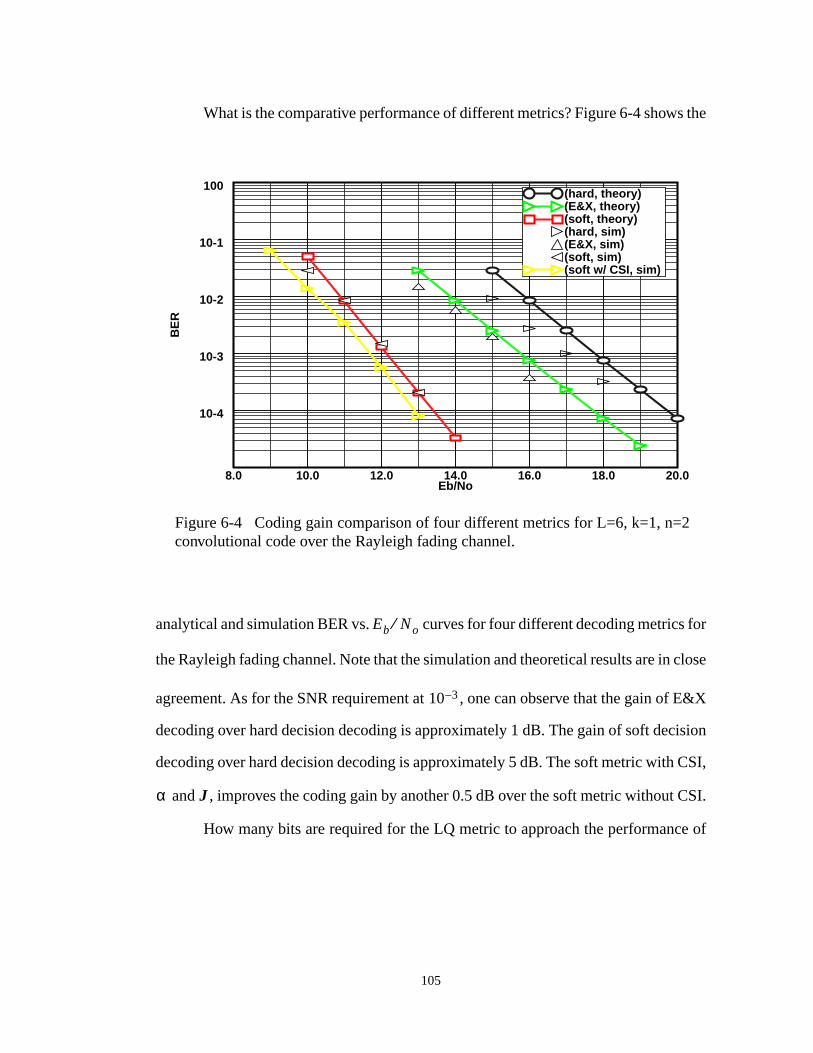
TABLE OF CONTENTSLIST OF FIGURES.................................................................................... vii
LIST OF TABLES........................................................................................ x
ACKNOWLEDGMENTS .......................................................................... xiii
VITA ..............................................................................................................
ABSTRACT OF THE DISSERTATION ................................................ xvii
Figure 6-13 Cutoff rate vs. SNR per bit for four different decoding
metrics with a NC-BFSK system over Rayleigh fading
bi-level, partial-band jammer channel (f=0.90,
Eb/No=13 dB). 116
Figure A-1 19 Hexagonal Cell Layout (Frequency Reuse Factor of
1/3) 122
Figure A-2 Hopping pattern by Latin-square construction (n = 8 and
frequency reuse factor of 1/3). 123
xi
xii
LIST OF TABLES
Table 4-1 Call blocking and call dropping probabilities with and
without distributed admission control for a single-cell
network 59
Table 4-2 Call blocking and call dropping probabilities with and
without distributed admission control for a single-cell
network59
Table 4-3 Call blocking and call dropping probabilities with and
without distributed admission control for a multi-cell
network 61
Table 4-4 Call blocking and call dropping probabilities with and
without distributed admission control for a single-cluster
network 62
Table 5-1 Code performance and delay comparison 71
Table 5-2 Eb/No at Pb = 10-3 for different decoding metrics for a
dual antenna diversity system. 79
Table 5-3 Code performance for different decoding methods81
pest
A. I
my
in the
Dr.
ive
Dr.
our
olas
any
Kim,
short
and
Pai,
ACKNOWLEDGMENTS
To my advisor, Professor Gregory J. Pottie, I would like to express my dee
gratitude for his guidance, support, and kindness throughout my years at UCL
am especially grateful for the extra time and effort he has devoted to shape
research experience and to ensure me continuing successful endeavors
engineering field.
I would also like to thank the other members of my dissertation committee:
Kirby Baker, Dr. Kung Yao, and Dr. Henry Samueli. I appreciate the collect
enthusiasm they have shown toward my research. Additional thanks go to
Samueli for providing me a rewarding consulting assignment with Broadcom.
To all the members of the radio transceiver project, I thank you for y
collaboration. I am grateful for the assistance of Dr. Tim Chen and Prof. Nich
Bambos in the study on power control issues. I am also thankful for the m
helpful technical discussions with my colleagues: Chris Hansen, Jaeheyong
Jonathan Min, Eldad Perahia, Ben Tang, and Charles Wang. The follow is a
list of colleagues and friends who made my stay at UCLA more interesting
enjoyable: Bruce Kwan, Steve Chin, Tom Kwon, Jeff Putnum, Eric Berg, Pat
xiii
ogize
the
h. I
ness
ing
ped
and
have
yers
Robin Joshi, Gordon Yee, James Chang, Glenn Chang, and Kirk Chang. I apol
for leaving anyone out inadvertently. I appreciate the help and efficiency of all
staff members in the Electrical Engineering department.
I would like to thank my extended family at the University Presbyterian Churc
thank especially Pastor Soon Chang and Esther Chung, for their warmth, kind
and prayers. I thank God that they have strengthen my faith in Him.
Lisa, I want to thank God for bring her into my life. She has shown me the mean
of love and spiced my life with laughters. I will always remember how she hel
me regain strength and focus when I felt heavy with burdens.
Most of all, I am indebted to my parents for their immeasurable care, support
understanding. Thank God for giving me parents who are so loving and wise. I
been deeply touched by my brother Tom and sister Cathy for their constant pra
and encouragement. Thank God for them and their families.
Lastly, I would like to acknowledge financial support from ARPA.
xiv
at-umss
lessory,
VITA
January 7, 1967 Born, Taipei, Taiwan
1989 B.S., Electrical EngineeringCornell UniversityIthaca, New York
1989-1990 Product Development EngineerHewlett PackardAndover, Massachusetts
1991 M. Eng., Electrical EngineeringCornell UniversityIthaca, New York
1990 Teaching AssistantCornell UniversityIthaca, New York
1992-1995 Research AssistantUniversity of California, Los AngelesLos Angeles, California
1994 Independent ConsultantBroadcom CorporationLos Angeles, California
PUBLICATIONS AND PRESENTATIONS
J. Min, A. Rofougaran, V. Lin, M. Jensen, A. Abidi, G. Pottie, and Y. RahmSamii, “A Low-Power Handheld Frequency-Hopped Spread SpectrTransceiver Hardware Architecture,” Virginia Tech Symposium on WirelePersonal Communications, Blackburg, VA, p. 10/1-8, June 1993.
V. S. Lin and G. J. Pottie, “Channel Coding for a Frequency-Hopped WireTransceiver,” Proc. of the 1993 Canadian Workshop on Information TheOttawa, Canada, pp. 109-124, 1994.
xv
ionnal
ngn
V. S. Lin and G. J. Pottie, “Implementation of Distributed Power and AdmissControl for a Frequency-Hopped Wireless Transceiver,” InternatioWireless ‘95 Conference, July 1995.
V. S. Lin and G. J. Pottie, “Adaptive Decoding Metrics with Convolutional Codiin FH/CDMA Systems,” Submitted to IEEE Transaction oCommunications
xvi
ction
ion
me
f the
ith
istic
the
ystem
te the
on
n are
hen
ABSTRACT OF THE DISSERTATION
Channel Coding and Power Control For FH/CDMARadios
by
Victor Shiaw-Jong Lin
Doctor of Philosophy in Electrical EngineeringUniversity of California, Los Angeles, 1995
Professor Gregory J. Pottie, Chair
We investigate the issues of adaptive power control, channel code sele
and decoding metrics formulation for a slow frequency-hopped/code divis
multiple access (SFH/CDMA) radio.
We show how to effectively adapt a distributed power control sche
proposed for single-channel narrowband systems to the unique constraints o
SFH/CDMA system. In addition, the performance of distributed power control w
a fixed transmit power dynamic range is studied through simulation. Heur
admission control algorithms for mitigating performance degradations due to
dynamic range constraints are presented. Some of the trade-offs between s
capacity and complexity are discussed.
We also present a low-delay channel coding technique and demonstra
benefits of dual antenna diversity in combination with coding. BCH, Reed-Solom
(RS), and convolutional codes are considered. The basis for code compariso
the system performance, delay and decoder complexity. It is shown that w
xvii
, the
idth
ision
g for
. For
g is
lass
ding
evel
nds
ition
ch as
imple
binary non-coherent FSK modulation and hard decision detection are used
BCH, RS, and convolutional codes that can meet the delay and bandw
constraints have similar performance and comparable complexity. Soft dec
decoding for the convolutional code and error-and-erasure correction decodin
the RS code are investigated in terms of the performance-complexity trade-offs
convolutional codes, it is shown that improvement over hard decision decodin
significant when the right decoding metric is selected.
To improve the effectiveness of coding in SFH/CDMA systems, a new c
of decoding metrics is formulated. The performance of new adaptive deco
metrics for convolutional codes is analyzed under Rayleigh fading and bi-l
partial-band noise jamming. New tighter probability of error performance bou
are derived. We find that adapting the metric according to the channel cond
provides significant performance gain over standard fixed decoding metrics, su
the soft decision and erasure and error decoding metrics. We also describe a s
algorithm for adapting the decoding metric.
xviii
rsed
ceiver.
e and
power
ignal
good
ased
over
ms
ents.
urces
annel
Chapter 1
INTRODUCTION
Wireless personal communication systems enable geographically dispe
users to exchange information using a portable terminal, such as a handheld trans
Often, the system engineer’s design objective is to maximize the transmission rat
number of simultaneous users (capacity) under the constraints of robustness,
consumption and hardware complexity. The tradeoffs among capacity, reliability, s
power, and cost of equipment can be complex. The topic of this thesis is a study of
system tradeoffs in wireless transceiver design.
Future generations of wireless personal communication systems will be b
on digital transmission technology. Digital technology has important advantages
traditional analog technology. With digital technology, radio communication syste
can be designed to meet more stringent transmission reliability requirem
Furthermore, digital technology enables more efficient sharing of channel reso
when multiple users need to access the system through a common ch
simultaneously.
1
ns?
897,
the
een
e new
the
red in
blic
etter
rove
and
built,
ne
n
lular
rvice
can
g and
first
fy the
1.1 Historical Perspective
What are some important milestones in the history of wireless communicatio
The birth of wireless communication is generally accepted to have occurred in 1
when Marconi received credit with the patent for the radiotelegraph, from which
word radio was coined [17]. Since that time, mobile radio communications has b
used to navigate ships and airplanes, dispatch police cars and taxis, generat
businesses, and win wars.
The use of radio telephones has evolved rapidly and grown explosively in
last few decades. This evolution of wireless systems can be viewed to have occur
different stages [19]. The main force driving the evolution is an increasing pu
demand for wireless services. To meet this ever increasing demand, b
communication technologies are required to increase network capacity, to imp
quality of service, and to introduce new service features.
The first generation of public wireless systems was developed in the 1970’s
the 1980’s, based on analog technology. During this period, several systems were
including Nordic Mobile Telephone (NMT) by Ericsson, Advanced Mobile Pho
Service (AMPS) by AT&T, and Mobile Cellular Service L1 (MCS-L1) by Nippo
Telephone and Telegraph (NTT) [17]. In order to improve system capacity, the cel
concept [14] was adopted. The main concept of cellular systems is that the se
region is divided into smaller areas, called cells. By using more cells, the system
support more users. To further improve capacity, other ideas, such as cell splittin
sectorization, were developed.
As the public appetite for wireless services gets bigger, the capacity of
generation systems, even with improvements, soon became insufficient to satis
2
digital
y is
alog
loped
and
stem
ed
spread
boost
read
tly in
aced
In
onal
over
nnot
ing
arent
ations
first
acity
e [7].
demand in some areas. This led to the development of the second generation
wireless system, built in the 1980’s and the 1990’s. In this period, digital technolog
implemented to improve the system capacity several times over traditional an
systems. At this stage, vehicular cellular radio and cordless telephone are deve
and optimized separately to provide service to users with different mobility patterns
communication needs [8]. The typical vehicular radio systems include Global Sy
for Mobile Communications (GSM) in Europe and Digital AMPS (IS-54) in the Unit
States; the typical cordless telephone systems include CT-2 in Europe and some
spectrum products in the United States.
Among second generation systems, one of the new technologies used to
system capacity is code division multiple access (CDMA). CDMA, based on sp
spectrum technology, is developed to utilize the available spectrum more efficien
multicell networks. The history of spread spectrum (SS) communications can be tr
all the way back to its military origin during early phases of World War II [36].
military applications, spread spectrum technology is used to combat intenti
jamming by an enemy transmitter. The approach to defeat jamming is to transmit
many signal coordinates with large-bandwidth signals, such that the jammer ca
achieve large jammer-to-signal power ratio in all the coordinates. The antijamm
properties of SS signals are well investigated and documented [37].
Since spread-spectrum uses large-bandwidth signals that result in the app
inefficient use of the radio spectrum, people had assumed that commercial applic
of SS radios were impractical [42][43]. Cooper and Nettleton, in 1978, were the
ones to recognize that digital spread-spectrum radio had a potentially higher cap
for mobile radio applications than the analog narrowband radios used at that tim
More research on digital SS mobile radio soon followed in 1980 [13][39].
3
ated
trum
d for
the
ead
ents.
read-
key
/SS)
ard,
ffice
dless
deral
trum
dio is
a more
ation
ey
tems
ility
lower
obust
of the
By the late 1980’s and early 1990’s, advances in very-large-scale integr
circuit (VLSI) technologies has made low-cost implementation of spread-spec
radio possible while the popularity of mobile radio has spurred the market deman
high-capacity systems. These factors contributed to a renewed interest in
application of spread-spectrum technology for mobile radio. The widespr
commercial development of SS wireless systems today is sparked by two key ev
One of the events is the 1985 FCC ruling which allows the unlicensed use of sp
spectrum radio in ISM bands, which include the 902 to 928 MHz band. Another
event is the well-publicized Qualcomm direct sequence spread-spectrum (DS
CDMA system which has led to the adoption of a second U.S. digital cellular stand
IS-95 [12].
Today, commercial spread-spectrum radios are used in indoor o
applications, such as wireless local area networks (WLANs), and wireless cor
phone (PBX) systems. Among the interesting outdoor applications is the Fe
Emergency Management Agency’s (FEMA) experimental use of spread-spec
radios to transmit digital video. In some situations, unlicensed spread spectrum ra
used as an emergency backup to wired lines and in many cases, they are used as
economical substitute for digital leased lines.
Numerous sources have projected that the demand for wireless communic
services will continue to grow rapidly well into the next century. One of the k
ingredients needed in third generation wireless personal communications sys
(PCS) is a low-power wireless access technology. The portability and affordab
requirements forces a design focus on power reduction to extend battery life and
component costs. Developing a low-power handheld transceiver that can provide r
wireless communications presents many technical challenges. To meet some
4
the
less
from
ation
igh
ystem
ltiple
tion
ding
ions.
ower
smit
ment
ith
elay
ation
tions
nnel
ition
as the
challenges, the UCLA personal communications project began in 1991.
1.2 Scope of Thesis
This thesis arises from work we have performed to develop and validate
system design techniques proposed for the UCLA prototype all-CMOS wire
transceiver handset. A radio signal propagating in a wireless environment suffers
severe corruption due to various channel impairments, making reliable communic
difficult. To overcome the radio channel impairments without resorting to h
transmitter power, the proposed architecture incorporates many advanced s
techniques, such as antenna diversity, slow frequency-hopped/code division mu
access (SFH/CDMA), channel coding, and adaptive power control.
The topic of this thesis is the study of the system tradeoffs in the implementa
of adaptive power control, channel code selection, and the formulation of deco
metrics for frequency-hopped transceivers in wireless communication applicat
Our investigation has resulted in the specification and validation of a distributed p
control scheme for a SFH/CDMA system, the determination of the sufficient tran
power dynamic range to prevent significant system capacity loss and the develop
of heuristic algorithms for reducing call dropping in a power controlled network w
dynamic power range restrictions. We have also performed a study on low-d
channel coding and demonstrated the benefits of dual antenna diversity in combin
with coding. In addition, we have designed an adaptive metric that can track varia
in channel statistics and a simple algorithm for adapting the metric to changing cha
conditions. We will show that adapting the metric according to the channel cond
provides significant performance gain over standard fixed decoding metrics, such
soft decision and erasure and error decoding metrics.
5
ion
e a
4 to
n of
ted
ts of a
ncy-
are
6 we
ghter
s for
Chapter 2 gives an overview of terrestrial cellular radio communicat
technologies, with particular attention to CDMA systems. In chapter 3 we outlin
framework and describe system models for analyzing CDMA systems. In chapters
6, we present our new results. In chapter 4 we consider the implementatio
distributed adaptive power control. We show how to effectively adapt a distribu
power control scheme proposed for narrowband systems to the unique constrain
SFH/CDMA system. In chapter 5 we consider channel coding options for a freque
hopped system employing NC-BFSK signaling. Alternative channel codes
compared on the basis of delay, complexity, and bandwidth efficiency. In chapter
propose new adaptive decoding metrics for convolutional code and derive new ti
probability of error bounds. Chapter 7 contains our conclusions and suggestion
future research.
6
usly
s to
ation
e to
these
and
adio
s have
efly
tem
gives
t are
Chapter 2
TECHNICAL BACKGROUND
In a multi-user radio communication system, several users can simultaneo
exchange information over different radio links. The system design objective i
establish as many reliable links as possible over an unreliable shared communic
medium. The principal impairments in a single link or channel are attenuation du
multipath fading and multiple access interference from other radios. To overcome
impairments, advanced digital transmission techniques are needed.
In this chapter, we outline basic multi-user radio system design principles
techniques. Specifically, we are concerned with the design of digital mobile r
systems based on spread spectrum technology. Spread spectrum technique
with non-ideal bandpass filters, transmit power will leak into the adjacent freque
bands. If the leakage power is significant in the system of Figure 3-1, link 1 and 2 w
emit adjacent channel interference to each other during every first and fourth time
in a frame. Although this example involves a peer-to-peer system, the latin-sq
construction can be similarly applied to cellular networks.
3.3 Radio Link Model
Within the network, there are many links. Figure 3-2 outlines the system mo
for a single radio link. The input bit stream is encoded and fed to the interleaver.
interleaver rearranges the coded sequence in such a way that the fading chann
burst error characteristic is transformed into a channel having independent errors
coded symbol at the output of the interleaver is transmitted by binary orthogonal
signaling. The frequency hopping binary FSK signal is output from a frequency ho
where the hopping local signal is multiplied by the binary FSK signal. A slow freque
EncoderBinary FSKModulation
Hopping FrequencySynthesizerSequence
Fading Channel
Hopping FrequencySynthesizerSequence
Decoder Binary FSKDemodulation
binarydata
binarydata
Deinterleaver Equal GainCombining
Interleaver
Figure 3-2 System Model.
ChannelEstimator
21
a few
tics of
band
e the
tenna
und
ot be
iver
ining
s have
on
an be
pread
y can
- time
hese
n the
om
annel,
ultiple
hop scheme is assumed in which a hop is made in each slot interval consisting of
symbols. The transmitted signal passes through a radio channel, the characteris
which are described in the next section.
At the receiver end, the received signal is first dehopped to obtain the base
binary FSK signal. Non-coherent detection is used for the reception, becaus
handheld system is designed to allow fast hopping. The receiver employs dual an
diversity with postdetection equal gain combining to achieve diversity. This was fo
to outperform selection diversity, and in any case when the channel SNR cann
estimated with any accuracy for a slot (e.g., fast hopping), two complete rece
branches are required to make antenna diversity effective. Thus, equal gain comb
comes essentially for free. We assume that the signals received at the two antenna
low correlation.
3.4 Fading Channel Model
An active radio link will experience transmission impairments. Depending
the bandwidth of the signal relative to the coherence bandwidth, channel models c
classified as wideband or narrowband. In the proposed SFH/CDMA system, the s
bandwidth is much larger than the coherence bandwidth so that frequency diversit
be achieved. However, the aggregate channel resource defined by the bandwidth
product is divided evenly into subchannels, as illustrated in Section 3.2, and t
subchannels are more like narrowband channels; hence, we will concentrate o
characterization of narrowband channels.
In classical AWGN channels, the signal is corrupted by an additive rand
signal, known as noise. When a signal passes through a multiple access radio ch
besides noise, other random processes, namely propagation phenomena and m
22
ssion
ts can
ath
at a
ations.
n be
. As
the
ables
sited
istic
ignal,
used.
zed
ding
s than
of a
ned as
access intereference distorts the signal. In this section, we will explain the transmi
impairments due to propagation and interference and show how these impairmen
be modeled for different types of performance evaluations.
3.4.1 Propagation Models
A major propagation mechanism in terrestrial mobile radio channel is multip
fading. Multipath refers to the many paths by which signal energy may arrive
receiver. The paths are characterized by different delays, phase shifts, and attenu
The low-pass equivalent impulse response of the multipath radio channel ca
modeled by a time-varying linear filter:
(3.1)
where the -th path has amplitude , phase and propagation delay at time
a signal is transmitted through a radio channel, physical characteristics of
propagation environment might be constantly changing. For example, the port
might be moving amongst natural or man-made obstacles which are are randomly
on irregular terrain. It is too complicated and unrealistic to pursue an exact determin
approach to modeling the propagation effects. To determine the received radio s
which may be influenced by many random factors, a statistical approach is often
The time-varying distortion caused by multipath fading is often characteri
by two kinds of spreading: delay spreading (spreading in time) and Doppler sprea
(spreading in frequency). Delay spread measured in indoor settings is usually les
100 ns [9]. For an outdoor microcellular environment, delay spreads on the order
few microseconds have been observed. The coherence bandwidth, which is defi
h t τ,( ) αi t( )eθi t( )δ t τi–( )i
∑=
i αi θi τi t
23
r than
ignal
the
is, all
phase
sed in
For
ad so
tive
time
based
ed as
r than
ps/
the
gnal
signal
The
ived
vel.
the inverse of the delay spread, ranges from around 1 MHz in outdoors to greate
10 MHz in indoors. For the proposed SFH/CDMA system, the instantaneous s
bandwidth is less than 1 MHz. When signal bandwith is narrow relative to
coherence bandwidth of the channel, the channel is frequency-nonselective. That
of the frequency components in the signal undergo the same attenuation and
during transmission. The impulse response for a narrowband channel can expres
the form:
(3.2)
This flat-fading channel results in multiplicative distortion of the transmitted signal.
such narrowband systems, the symbol period is much longer than the delay spre
that intersymbol interference (ISI) is negligible and ISI reduction by adap
equalization is unnecessary. Doppler spread due to terminal motion causes
variations in the envelope of the received narrowband signal. For a pedestrian
system, the doppler spread is small (e.g 5 Hz). The coherence time, roughly defin
the inverse of doppler spread, is approximately 0.2 seconds, which is much greate
the frequency dwell time of SFH/CDMA system (e.g. 6 at the hop rate of 160 kho
s). This implies that the channel fades relatively slowly, the condition under which
multiplicative distortion may be regarded as a constant within a hop.
For the purpose of predicting the received strength for a narrowband si
at a receiver, we use a propagation model that quantifies the phenomena of
propagation by two factors: the median signal strength, and the signal variability.
prediction is a two step method involving an estimation of both the median rece
signal within a relatively small area, and the signal variability about the median le
h τ t,( ) α t( )eθ t( )δ t τ–( )=
µs
α t( )
24
the
iction
The
sured
fects
, the
ance
ength,
t. The
ath
which
lly a
oving
ance
at 30
hin a
tween
ns of
3.4.1.1 Median Signal Strength
There are a number of models described in the literature for predicting
median signal strength in a small area [27]. In general the models used in the pred
methods are a mixture of empiricism and the application of propagation theory.
empirical approach relies on fitting curves or analytical expressions to sets of mea
data and implicitly attempting to take factors such as diffraction, atomospheric ef
or irregular terrain into consideration. When the signal variability is averaged out
path loss has been empirically determined to follow an inverse power law with dist
between the transmitter and receiver. That is, the average received signal str
denoted by , can be written as:
(3.3)
where is called the path loss exponent, is the distance, and is some constan
values of ranged from 1.5 to 6, depending on the propagation environment.
3.4.1.2 Signal Variability
It is often useful to separate the effects of signal variability due to multip
fading on a basis of scale into those which occur over a short distance and those
are apparent only over much longer distance. Although fading is fundamenta
spatial phenomenon, it is experienced as a temporal variation by a receiver m
through the multipath field. Local multipath that can be observed over a short dist
on the order of a wavelength causes short-term fluctuation. For a receiver moving
miles/hour, several short-term fades, also known as rapid fading, can occur wit
second. The long-term variation, caused by gross changes in the overall path be
the transmitter and receiver, occurs over much larger distances on the order of te
Γ r( )
Γ r( ) Ar γ–=
γ r A
γ
25
to the
rchers
ed by
iation
with
the
nity
rem
zed as
lows a
ility
for
term
-term
nce
wavelengths. Because the variations are often caused by the mobile moving in
shadow of buidlings or hills, long- term fluctuation is called shadowing.
When shadowing is present, measurements reported by several resea
[30][15][2]suggest that the average received signal strength at distance , denot
, has the log-normal distribution:
(3.4)
where all units are in decibles. For similar environmental areas, the standard dev
has been observed to be independent of path length. It ranges from 4-18 dB,
being a typical value for urban environments.
The signal variability also has a rapid fading component superimposed on
log-normal variation. This is caused by multipath propagation in the immediate vici
of the receiver. In the absence of a strong line-of-sight path, the central limit theo
arguments may be invoked to show that the received waveform can be characteri
a complex Guassian process. The envelope of a complex Gaussian process fol
Rayleigh distribution and the phase follows a uniform distribution. The probab
density function of Rayleigh fading can as written as:
(3.5)
where , the second moment, represents the average signal power.
The distinction in time scales of the signal variability is extremely useful
engineering. Mathematically, this means that the statistical model of the short-
fading is conditioned upon the instantaneous values of the parameters of the long
statistics [31]. For most fading channels, only the short-term fading variations influe
r
Γ r( )
pΓ r( ) x( )1
2πσ--------------exp x Γ r( )–( )2
2σ2--------------------------–
=
σ 8=
f y( )y
σ2------exp y
2σ2---------–( )=
2σ2
26
the
he
ues
g in
kage
rence
noise,
sired
s, log-
at all
to
deled
any
next
nmit
on.
easing
d. To
the selection of the appropriate method of modulation, diversity, and coding; only
long-term fading variations determine the availability of the channel. T
dichotomization of the time scales allows us to analyze network and link iss
separately. We will elaborate the practical implication on propagation modelin
Section 3.5 and Section 3.6.
3.4.2 Interference Model
Frequency reuse leads to co-channel interference while spectral lea
produces adjacent-channel interference as described in Section 3.2. The interfe
and desired signals arrive simultaneously at a receiver and, excluding the thermal
their sum is the received signal. Since the interference signals, similarly to the de
signal, pass through the propagation channel, they are impaired by distance los
normal shadowing, and Rayleigh fading. In modeling interference, we assume th
signals are affected by independent but identical statistics.
As with propagation modeling, proper modeling of the impairments due
interference must match the engineering interest. Interference signals can be mo
individually or as a single aggregate process, resulting from the combination of m
signals. How to choose the right model for a specific purpose is discussed in the
two sections.
3.5 Channel Modeling for Power Control Study
In CDMA systems, power control techniques are employed to adjust the tra
power from every radio link to the minimum level required for reliable transmissi
This saves power and also reduces the interference in nearby cells, thereby incr
capacity. Power control algorithms can be classified as centralized or distribute
27
ations,
On
ally.
and
d and
t of
s be
thm
k to
loss.
hold,
iable
-loop
hat an
d by
access
both
ge
l, an
n it
rence
tem
implement centralized algorithms, there must be some terminals, such as base st
that can cooperatively control the transmit power of every radio link in the network.
the other hand, under distributed algorithms each radio link adjusts its power loc
Distributed power control is suitable for peer-to-peer systems, such as military
emergency response applications in which base stations may not be deploye
centralized control is impractical. Futhermore, it is desirable from the practical poin
view of avoiding burdening higher levels of the network even should base station
available.
Chapter 4 studies the implementation of a distributed power control algori
for the proposed SFH/CDMA system. The power control algorithm uses feedbac
deal with slowly varying channel conditions, namely shadowing and free space
The algorithm adapts with respect to an average signal-to- interference (SIR) thres
reducing the average transmitted power to the level actually needed for rel
transmission. Power control with respect to a SIR measure requires a closed
structure whereby the two parties on occasion exchange messages indicating t
adjustment in transmitted power level is required.
Power control is mainly a network issue. Its effectiveness can be measure
system capacity, often defined as the number of users that can simulatenously
the system with some guaranteed quality of service. Quality of service is related to
reliability and availablility requirements. Reliability is usually a function of avera
SIR. By keeping the mean SIR near a desired threshold through power contro
implicit reliability requirement is established. A link is considered unavailable whe
cannot obtain the SIR threshold, which occurs when there is excessive interfe
from other co-channel users in the system.
One purpose of studying power control algorithms is to determine sys
28
er
ithm
the
ws
ystem
ften
nnel
log-
long
iver
the
sion
e a
d in
for
ains:
any
l code
ance,
, and
ally
availability as a function of network loading. In addition, the dynamics of the pow
control algorithm are interesting. Knowing the convergence property of the algor
is very important. Since power control involves interaction between multiple links,
interference model should treat the signal in every radio link individually. This allo
changes in SIR over succesive slots and frames to be determined. Since the s
model for studying power control is highly complex, a simulation approach is o
required to examine the system behavior. For power control simulations, a cha
model should include slowly varying propagation effects, namely distance loss and
normal shadowing, on the individual signals. The rapid fading can be ignored as
as we assume perfect channel measurements.
3.6 Channel Modeling for Channel Code Study
The power control mechanism in the proposed SFH/CDMA transce
architecture can overcome slowly changing channel impairments. However,
proposed power control algorithm cannot deal with the other dominant transmis
impairments in SFH/CDMA systems, namely multipath fading. In order to achiev
high capacity with low power consumption, it is essential that diversity be employe
the transceiver architecture. There are many well-known diversity techniques
mitigating rapid fading. These techniques can be realized into one of three dom
space, frequency, and time. Channel coding provide time diversity. There are m
different channel codes and one of the issues in transceiver design is channe
selection. The selection process considers tradeoffs among error perform
transmission delay, channel bandwidth expansion due to added redundancy
algorithmic complexity.
The effects of rapid fading on communications performance are usu
29
SNR.
as an
d the
annel
at the
or of
nges
ce.
vere
w the
good
tion
ds on
ance
odel
log-
rent
rror
ents
described by the error-rate performance of the transceiver as a function of mean
In link performance simulations, the total inteference statistics could be modeled
additive white Guassian process. When there are many significant interferers an
transceiver employs frequency hopping, long interleaving span and a powerful ch
code, the randomized interference will appear as an additive white Gaussian noise
baseband. The AWGN might have a time-varying variance to simulate the behavi
fading interferers. The variance of the noise might also be time varying due to cha
in system loading, which could lead to increase or decrease in system interferen
3.7 Summary
In radio communications, the channel is highly complex and causes se
degradation to the transmitted signal. It is important to understand and model ho
channel places fundamental limitations on the performance of the system. A
channel model can facilitate the design and development of radio comunica
techniques for achieving robust transmission. Choosing a channel model depen
many factors, such as the signal characteristics and the goals of the perform
analysis.
In general, for the purpose of determining system availability, a channel m
might include the slowly-varying propagation effects such as distance loss, and
normal shadowing. The model need to include all the various signals in the diffe
links in the system. On the other hand, for the purpose of computing bit e
performance on a single link the channel model could consists of only the impairm
due to rapid fading and AWGN.
30
biles
. For
ted
mple,
the
the
MA
rithm
n the
e for
ing
Chapter 4
IMPLEMENTATION OF
DISTRIBUTED POWER CONTROL
Dynamic control of the transmit powers and channel assignments of the mo
in a wireless network can greatly improve system capacity and resource allocation
networks requiring reduced complexity of protocols and infrastructure, distribu
power control schemes are more appropriate than centralized ones. For exa
distributed power control could be used in peer-to-peer networks which eliminate
complexity associated with base-stations. In this chapter, we describe
implementation of a distributed power control scheme for the prototype SFH/CD
system. The scheme is based on a distributed power and admission control algo
developed by Chen et. al [4]. An important feature in their scheme is the protectio
operational links by suppressing new links that may cause the quality of servic
ongoing calls to fall below a certain target.
In this chapter, we present capacity analysis of different networks, assum
31
ed
des a
ing
. A
deals
vide
with a
thms
s are
int
rage
ot be
els,
in a
f the
bels.
tage
power control with limited dynamic range. Some analytical results for simplifi
systems are presented to verify simulation results. The idealized system provi
baseline for comparison against more realistic systems.
The chapter is organized as follows. In Section 4.1, the motivation for study
distributed power control with dynamic range constraints (DPCDRC) is given
mathematical description of DPCDRC is presented in Section 4.2. Section 4.3
with capacity calculation of systems with different power control schemes to pro
some benchmarks for comparison. Section 4.4 studies performance degradation
dynamic range constraint and details the problem of dropped calls. Heuristic algori
for reducing dropped calls are presented in Section 4.5. Finally, concluding remark
made in Section 4.6
4.1 Motivation
The following simple example illustrates how a dynamic range constra
affects the outage probability of a network. Outage probability is defined as the ave
fraction of the service area over which an acceptable transmission quality cann
maintained [34]. We take this as our principal measure of performance.
In the network of Figure 4-1, there are two links operating in adjacent chann
both receivers are fixed at the origin, and the transmitters are uniformly distributed
unit circle centered at the origin.
Let the adjacent channel interference emitted from a transmitter be o
power in the transmitter’s own channel. Define as the dynamic range in deci
When the SIR of a link drops below the acceptable threshold, denoted by , ou
occurs. That is,
α dB
x
γ
32
l.
r law
utage
hen
iven
ed
(4.1)
where = power of the desired signal, and = power of the interference signa
Assuming that radio propagation attenuation obeys an inverse fourth powe
with distance, we can derive a relationship between the distances under the o
condition:
(4.2)
Let and be modeled as random variables with uniform distributions, t
the outage probability is given by
(4.3)
where
(4.4)
Figure 4-2 plots the analytical result for a variety of dynamic range values, g
and . The -29 dB interference rejection factor is determin
d2
d1
tx
rx1 and rx2
int
Figure 4-1 Simple example with two links
SIR Pr Pi– α– x+ γ<=
Pr Pi
d2 10
γ α x–+( )40
--------------------------
d1≤
d2 d1
P d2 kd1– 0<{ } dxdy
0
ky
∫0
1
∫=
0.5k; k 1≤=
k 10
γ α x–+( )40
--------------------------
=
γ 12 dB= α 29 dB–=
33
ng
the
hing
city.
th the
in
e of
FH/
IR)
s of
from a functional simulation of the UCLA prototype SFH/CDMA transceiver, taki
into account the frequency responses of the transmit and receiver filters.
The plot exhibits a general trend in which more dynamic range reduces
outage probability, and also that increasing the dynamic range yields diminis
improvements in the outage probability, which is related to the system capa
Simulation results (marked by rectangles) for this simple case are in agreement wi
analytical result. Next, we consider more realistic networks.
4.2 Description of Power and Admission Control
Algorithm
A general description of the system models for SFH/CDMA network is given
Chapter 3. Here we provide additional details about the models for the purpos
studying power control issues. To implement distributed power control over a S
CDMA link, we must be able to reliably estimate the signal-to-interference ratio (S
at the receiver. Unreliable SIR information can significantly reduce the benefit
20.0 30.0 40.0 50.0Dynamic Range (dB)
0.010
0.020
0.030
0.040
0.050P
out
Figure 4-2 Outage Probability vs. Dynamic Range for andγ 12 dB=
α 29 dB–=
34
nt a
f the
ten or
entage
hen
hich
nal is
e on
iven
e hops
annel
n. In
wly
ies on
for
f the
is
ality
power control. The non-coherent correlator outputs can be used to impleme
maximum-likelihood estimator for the SIR [49]. To obtain reliable measurements o
SIR, the estimator must average over hundreds of samples in a frame instead of
less samples in a hop. The RMS error in the SIR estimation, expressed as a perc
of the actual value, is approximately , where is the number of samples. W
the number of samples is greater than 100, the RMS error is less than 10%, w
implies a fairly accurate measurement of the SIR. Given the SIR estimate, a sig
sent to the corresponding transmitter to update the transmit power.
In our power control scheme, the power will be adjusted once per frame bas
a reliable measure of the “average” SIR, which is mathematically defined below. G
the transmit power is constant across a frame, the SIR can fluctuate in successiv
as multipath and the combination of links causing mutual interference change. Ch
coding is thus required to overcome hops with SIR too low for reliable transmissio
other words, our SFH/CDMA system uses power control to mitigate the slo
changing channel impairments such as shadowing and distance loss, and rel
channel coding to combat the rapid channel variations.
In order to study the power control problem with constrained transmit power
SFH/CDMA systems, we propose the following system model as an extension o
models in [10][24]. The performance object is to achieve
(4.5)
where is the SIR of the i-th link averaged over the N time slots within a frame,
the prefix SIR target value determined by the lowest acceptable global service qu
1 M⁄ M
Ri γ≥ i 1 2 … M, , ,=( )
Ri γ
35
n
al
s. The
d in
the
h
of the network, and M is the number of links.
In (4.5), is given by
(4.6)
where is the power transmitted by the ith transmitter, is the “average” attenuatio
between the ith transmitter and the jth receiver and is the power of the additive therm
noise in each receiver. We assume that all receivers have the same noise floor
average attenuation in (4.6) can be written as
(4.7)
where is the attenuation between the ith transmitter and the jth receiver during the
kth time slot within a frame. Equations (4.5) and (4.6) may be combined and state
matrix form along with the transmit power constraint as follows:
(4.8)
where is the vector of transmitter powers which are constrained to be within
interval , is the identity matrix, matrix is non-negative wit
elements:
(4.9)
Ri
RiGii Pi
Gij Pij i≠∑ η+-------------------------------=
Pi Gij
η
Gij1N---- Gij
k( )
k 1=
N
∑=
Gijk( )
I γF–[ ]P u≥PL Pi PU≤ ≤
P
PL PU,[ ] I M M× F
Fij 0 if i j==
Gij Gii⁄ if i j≠=
36
rve
e
is
eater
ect
uted.
ork
nt to
an
is
etting
and is the vector with elements
(4.10)
A solution to (4.8) is feasible if at least one solution vector exists. Obse
that the SFH/CDMA system model reverts to the original TDMA/FDMA model if w
let and . That is, (4.8) becomes
(4.11)
Mitra [24] showed that if a solution to (4.8) exists, then a particular solution
, where
(4.12)
and this solution is Pareto optimal in that any other which also satisfies (4.8) is gr
than . Note that finding the solution by (4.12) requires global control to coll
measurements of and the distribution of the power vector after it has been comp
Our objective as formulated in (4.8) is to use power control on a SFH/CDMA netw
to minimize transmitters’ powerswithin the dynamic range constraintswhile giving
each link enough power to satisfy their target average SIR and furthermore, we wa
do this in adistributed manner to reduce network control complexity.
Foschini [10] proposed a distributed power control algorithm based on
iterative power update approach using the power update equation:
(4.13)
Without any dynamic range restrictions, this simple distributed algorithm
guaranteed to converge to the Pareto optimal power solution, whenever a power s
u
γη Gii⁄= i 1 2 … M, , ,=(
P
PL PU,[ ] 0 ∞,[ ]= Gijk( ) Gij= , k∀
I γF–[ ]P u≥Pi 0≥
P*
P* I γF–[ ] 1– u=
P
P*
G
P n 1+( ) γFP n( ) u+=
37
tion
ted
ified
n be
sted
at the
ntrol
of
able.
onal
ional
er
our
The
screte
cess
are
exists for which all links meet the SIR requirement. That is, when there exists a solu
which can found by the global algorithm (4.12), the solution of the distribu
algorithm approaches it geometrically fast [24]. Chen, Bambos and Pottie [4] simpl
Foschini’s distributed algorithm and showed that the power update equation ca
rewritten as:
(4.14)
Equation (4.14) specifies that the current transmitter power should be adju
by a factor that is equal to the ratio of the target SIR to the measured average SIR
receiver.
Computing power updates is an essential part of the distributed power co
algorithm. In [4] a power update algorithm is developed to protect the quality
operational links when the set of desired SIR requirements are no longer achiev
The algorithm incorporates a non-linear adjustment function to allow the operati
links to increase their powers more rapidly than the new links so that the operat
links will always maintain their target SIR while the new links might end up with low
SIR. The power adjustments in [4] are drawn from a set of real numbers. For
implementation, however, we quantized the power update function to four levels.
steps were chosen to preserve the active link protection mechanism. By using di
adjustment levels, the control traffic in the feedback loop of the power control pro
is minimized.
Our modified update scheme is formalized below. Define
(4.15)
where the power update functions for an operation link i and a new link j
Pi n 1+( )γ i
Ri n( )------------Pi n( )= i 1 2 … M, , ,=( )
PidB k 1+( ) Pi
dB k( ) gi RidB k( ) γ i
dB ∆––( )+=
38
t the
.15),
by
SIR
rgin,
up.
wer
set
IR
track
links
tion
ile an
link
arget
given by (4.16) and (4.17), respectively.
(4.16)
(4.17)
The only difference between the first and second update function is tha
maximum step size is versus , where is a quantized adjustment step. In (4
a protection margin is provided by raising the effective SIR target of all links
approximately . In addition, the quantization adds a margin of so that the effect
is actually between and . Whenever its SIR drops into the protection ma
the operational link can increase its power faster than a new link that is powering
The protection margin can be optimized for fine tuning the performance of the po
control algorithm.
A simple admission control policy algorithm was also derived in [4]. When a
of SIR requirements become unattainable, a new link will see little or no S
improvements despite increasing its power. The basis of the admission policy is to
the changes in SIR relative to the increase in transmit power and block any new
with small SIR versus power slope in order to relieve network congestion.
When the transmit power is constrained, the admission control will malfunc
under certain circumstances. For example, suppose a new link powers up wh
operational link, denoted by O, is already at maximum power level. The new
generates interference to active users, causing the SIR of link O to drop below t
gi x( )
δ– x δ>0 0 x δ< <δ δ– x 0< <
2δ x δ–<
=
gj x( )
δ– x δ>0 0 x δ< <δ δ– x 0< <
=
2δ δ δ
∆ δ
∆ δ ∆+
39
line
get to
e it
that
out.
ant
re of
nnels
The
e-cell
rithm
link
timal,
. The
SIR
l sets
utage
bout
ing
SIR. Since link O can no longer increase its power, its transmission quality will dec
as the new link, which sees SIR improvements, continues to increase its power to
the target SIR. If the new link is admitted, link O will terminate prematurely becaus
can no longer maintain reliable transmission. Thus, failing to reject a new link
causes infeasible SIR requirements forces one or more operational links to drop
Since call dropping is a more annoying problem than call blocking, in general, we w
to keep the call dropping probability lower than the call blocking probability.
4.3 Network Capacity for Ideal Power Control
We use both the number of users per cell and slot efficiency as the measu
capacity performance. Slot efficiency is defined as the ratio of the number of cha
occupied to the number of available channels at a certain outage probability.
cellular systems in this section are assumed to have ideal power control. For singl
systems, we computed the optimum capacity using the global power control algo
given in (4.12). For multiple-cell systems, the power is controlled so that all reverse
signals are received at the same power level. Although the latter scheme is subop
it is computationally less expensive and the capacity analysis is more tractable
simulation procedure starts with no calls, and adds calls until the set of
requirements becomes infeasible. This is repeated for a large number of tria
(10000) so that the average efficiency of slot usage can be computed at an o
probability not exceeding 1%. The next section furnishes some additional details a
the SFH/CDMA simulation model.
4.3.1 Simulation Parameters
Our simulations include both cellular and clustered systems. The follow
40
ction
h
s)
r
in
in
ng a
assumptions apply to the parameters of the SFH/CDMA model described in Se
4.2:
1. All cells/clusters are of equal size and hexagonal shape. The radius of eac
hexagon is small enough to ensure the systems are interference-limited.
2. The location of portables (both transmitters and receivers in cluster system
is uniformly distributed within the coverage area.
3. All portables have a common antenna height and antenna gain.
4. Orthogonal hopping patterns are generated by a 32-element latin square;
hence, each cell/cluster can accommodate a maximum of 32 links. In othe
words, Nl = 32, where Nl is the maximum number of links per cell/cluster.
Both the number of orthogonal hopping tones and the number of time slots
a frame is also 32. That is, .
5. A common fourth-power path loss model is used to describe the signal
propagation for all transmitter-receiver pairs. All transmitted signals are
affected by log-normal shadowing with identical statistics.
6. Adjacent channel interference is specified by the ACI coupling factor.
According to the RF transmit and receive filter specifications of the UCLA
prototype SFH/CDMA system, the out-of-band emission to an adjacent
frequency is approximately 29 dB down from the peak transmitted power
the desired frequency.
7. Thermal noise can be modeled as a constant. It can be calculated assumi
NT N 32= =
41
na
g
SFH/
ell
ped
SNR
I, the
stem
ing
ame.
ACI
most
then
3 dB noise figure for the low-noise amplifier.
8. Perfect knowledge of the SIR parameters at a receiver is available to the
corresponding transmitter.
9. The established SIR requirement includes the gain from coding and anten
diversity. The effectiveness of antenna diversity and error correction codin
in mitigating multipath fading is demonstrated in later chapters.
Unless otherwise stated, the above parameters will be the standard for all
CDMA simulations. The next section deals with the basic SFH/CDMA single c
system, and the subsequent sections deal with multi-cell and clustered systems.
4.3.2 Single Cell Reverse Link Capacity
The single-cell capacity formula in [12] can be extended to frequency-hop
single cell systems utilizing an average power control scheme, in which the frame
is kept constant and the slot SNR may vary about the mean. When there is AC
hopping patterns are no longer completely orthogonal, and so a SFH/CDMA sy
will experience in-cell interference, similar to a DS/CDMA system.
The capacity of a single-cell SFH/CDMA system with well-designed hopp
patterns may be closely approximated as follows. First, find the average SNI per fr
where is the adjacency coefficient for the hopping pattern used and is the
coupling factor. In the best case, any pair of users will be in adjacent channels at
twice in each frame. If the hopping patterns has this optimum adjacency property,
SI--- S
N 1–( )Sxf η+-------------------------------------=
f x
42
the
is
e total
ited.
-cell
onte
acity
ent
n have
r user
it can be shown that
Then,
Finally, solve for N to obtain
(4.18)
where is the total spread spectrum bandwidth, is the information bit rate, is
desired signal power at the base-station, is the ACI coupling factor,
the per user average frame SNR requirement, and is the background noise in th
bandwidth, . The noise term can be ignored when the system is interference lim
We can look at as the effective processing gain with respect to the in
interference.
To compare the capacity approximation and the exact result obtained by M
Carlo simulation, we examined a 32-link system with an ACI coupling factor of
dB. Figure 4-3 shows that the analytical result accurately predicts the cap
performance.
We note that the simulation and analytical results are in close agreem
because the hopping patterns generated by a 32-element latin-square constructio
good adjacent interferer randomization. That is, most users interfere with any othe
f2RW-------=
Eb
No------
AVG
S R⁄I W⁄----------- S R⁄
2x N 1–( )S η+[ ] W⁄----------------------------------------------------= =
N
1 W R⁄2x Eb No⁄( )AVG
--------------------------------------ηS--- 1
2x------–+ if 2x Eb No⁄( )AVG 1>
W R⁄ otherwise
=
W R S
x Eb No⁄( )AVG
η
W
W 2xR( )⁄
10–
43
to a
ows
is
MA
lar
FH/
ach
. This
from the same cell only twice in each frame.
Capacity in terms of number of users per cell can be easily converted
corresponding slot-efficiency value. For example, at 9 dB SNR, the plot above sh
and since the number of available slots is 32, the slot-efficiency
.
4.3.3 Multiple Cell Reverse Link Capacity
It is easy to see that in the absence of ACI, a latin-square based SFH/CD
cellular system utilizing average power control is similar to a DS-CDMA cellu
system without the in-cell interference. Hence, the reverse-link capacity of a S
CDMA cellular system could be analyzed using the approach in [12]. This appro
assumes that the interference in the SFH/CDMA system has Gaussian statistics
5.0 6.0 7.0 8.0 9.0 10.0Eb/No
15.0
20.0
25.0
30.0
35.0
NW/R = 32
Simulation
Analytical
ACI = -10 dB
Figure 4-3 Reverse Link Capacity of the Single Cell SFH/CDMA
N 25=
21 32⁄ 0.66=
44
sers.
t of
ell,
ACI
BER
this
on
rger
assumption is valid when the interference is not dominated by a small number of u
In our analysis, we consider systems with and without ACI. Assuming the effec
thermal noise is negligible, the result is
(4.19)
where is the outage probability, and is the number of users per c
is the per user average frame SNR requirement and is the
coupling factor. Given that a certain is needed to achieve adequate
performance, (4.19) can be used to upper bound the probability of not achieving
level of performance for users/cell at any given time (e.g. 1% of the time).
Solving (4.19) for we obtain:
(4.20)
where is an upperbound on and is an upperbound
, which can be found by numerical integration. is defined as
(4.21)
Notice that (4.20) is a quadratic equation in , the number of users per cell. The la
P Pr I FRAME S⁄ δ>( ) Qδ mN–
σ N------------------( )==
δ
W R⁄Eb No⁄( )AVG
-------------------------------- if no ACI
W R⁄Eb No⁄( )AVG
-------------------------------- 2x N 1–( )– otherwise
=
P N
Eb No⁄( )AVG x
Eb No⁄( )AVG
N
N
m2N2 σQ
1–P( )( )2
2mW R⁄
Eb No⁄-----------------
+ N–
W R⁄Eb No⁄-----------------
2+ 0=
m E IFRAME S⁄( ) σ
var I FRAME S⁄( ) Q k( )
Q k( )1
2π---------- e x2 2⁄– xd
k
∞
∫=
N
45
the
city
ess
19 cell
ed in
MA
peer-
d on
root obtained from direct solution is the capacity.
Figure 4-4 plots the capacity expression for the SFH/CDMA system when
“processing gain” is 156. The analytical result shows that the effect of ACI on capa
performance is negligible in comparison to CCI when the ACI coupling factor is l
than -20 dB. We also observe that the analysis and simulation results based on a
network diverge for smaller values of N because the Gaussian approximation us
the analysis becomes less accurate.
4.3.4 Peer-to-Peer Cluster Capacity
This section presents the capacity of clustered peer-to-peer SFH/CD
networks described in Section 3.1. The lack of regular geometrical structure in a
to-peer network renders capacity analysis problematic at best. Hence, we relie
6.0 8.0 10.0 12.0 14.0Eb/No (dB)
0.0
10.0
20.0
30.0
40.0
50.0
N
Figure 4-4 Reverse-Link Capacity/Cell of the cellular SFH/CDMA system(with and without ACI. The ACI coupling factor is -20 dB).
Poutage = 0.01W/R = 156
Simulation
Analysis
46
ing of
e a
ctly to
s. The
the
his
hen
tems
. An
will
rence
tem.
ere
more
een
ome
m.
in the
uard
firms
uare
simulation to calculate the capacity of the standard model described in the beginn
Section 4.3. An algorithm is needed to organize links into clusters. We assum
situation where the algorithm has set up hexagonal boundaries that conforms exa
the ones in the cellular system. In each cluster, there are an equal number of user
simulation of a single-cluster network with our distributed algorithm shows that
slot-efficiency is approximately 6% at 1% outage probability when is 9 dB. T
performance figure is very poor in comparison to the 62% slot-efficiency found w
the network contains a base-station. (see Section 4.3.3).
The large disparity in performance between the clustered and cellular sys
indicates a fundamental trade-off between capacity and network infrastructure
intuitive benefit from having a base-station is that most of the time, a transmitter
transmit more signal power to the desired receiver than adjacent channel interfe
power to the other receivers. However, this is often not true in a clustered sys
Although the only source of interference comes from ACI, ACI could be a very sev
problem when the links are in a more random configuration.
One way to obtain reasonable capacity for peer-to-peer systems is to add
complexity by doing better frequency planning. For example, the guard band betw
different frequency slots can be increased to reduce ACI. This would trade-off s
spectral efficiency to improve the overall system capacity.
Figure 4-5 shows the effect of reducing ACI within the single-cluster syste
Suppose a larger guard band is introduced so that there are fewer channels
available bandwidth and that the ACI is reduced to -50 dB. Assuming that the g
bands takes up about half of the available bandwidth, then data in Figure 4-5 con
that a slot-efficiency of about can be achieved.
For multi-cluster systems we can combine frequency reuse with the latin-sq
γ
16 32⁄ 50%=
47
n be
H/
licit
ce for
is a
le-
construction to improve system capacity. Appendix A shows how latin-squares ca
modified for frequency-reuse with little additional complexity. In general, a SF
CDMA system does not require frequency planning but simulations show that exp
frequency- reuse is absolutely necessary to obtain reasonable capacity performan
multi-clustered systems. The computed slot-efficiency of a 19-cluster network
dismal 7.3% at 1% outage probability for a 9 dB SNRrequirement. The cost of the
frequency planning to make the entire network mobile can be quite high.
4.4 Performance Degradation Due to Power Control
With Dynamic Range Constraint
Although in the following sections we will focus mainly on the standard sing
-50.0 -40.0 -30.0ACI Coupling factor (dB)
0.0
5.0
10.0
15.0
20.0
N
Figure 4-5 Capacity of single-cluster SFH/CDMA system versus differentACI coupling factor
W/R = 32Eb/No = 9 dBPoutage = 0.01
48
MA
two
e that
pacity
the
hen
also
s are
will
the
the
mic
med
ctive
base-
d by
verse
table
ual to
cell SFH/CDMA system, analogous results can be obtained for other SFH-CD
network configurations. Insufficient transmit power dynamic range could result in
kinds of performance degradations. First, under a centralized power control schem
has a mechanism to block calls causing dynamic range problems, the network ca
could be lowered to compensate for additional blocked calls in order to maintain
original 1% outage criterion. Second, for a distributed power controlled system, w
there is insufficient dynamic range, one or more active calls may be dropped, which
contributes to the outage probability. From the customer’s viewpoint, dropped call
more of a nuisance than a slightly lower network availability. In Section 4.4.1, we
examine the loss in capacity from imposing a dynamic range constraint on
centralized power control algorithm. In the subsequent section, we will study
degradations in performance of the distributed power control algorithm when dyna
range constraints are imposed.
4.4.1 Global Algorithm with Dynamic Range Constraint
In deriving the theoretical capacities formulas (4.18) and (4.20), it was assu
that the portable’s transmit power dynamic range is sufficient to ensure that all a
portables, regardless of their locations, can deliver equal received power to the
station. Thus, it can be inferred that the dynamic range requirement is determine
the propagation model and the cell radius. Assuming the propagation loss is an in
4-th law with distance, the design rule for the dynamic range is simply:
(4.22)
where and are the maximum and minimum separations between a por
and the base-station, respectively. When the dynamic range is greater than or eq
DR* 40Rmax
Rmin-----------
log=
Rmax Rmin
49
log-
st be
tion
with
as a
mic
ws the
t can
at the
, the theoretical capacity predicted by (4.18) or (4.20) can be achieved. When
normal shadowing is included in the propagation model, the dynamic range mu
increased by some margin.
A Monte Carlo simulation was written to quantify the performance degrada
due to a limited dynamic range by computing the capacity of a single-cell network
a dynamic range less than . We will assume that the global scheme h
mechanism for blocking new calls to prevent dropped calls due to insufficient dyna
range. The other system parameters (e.g. the cell radius) are fixed. Figure 4-6 sho
simulation results. Capacity here is defined to be the maximum slot efficiency tha
supported at 1% outage probability. With these parameters, Figure 4-6 shows th
DR*
DR*
50.0 60.0 70.0 80.0Dynamic Range (dB)
0.0
5.0
10.0
15.0
20.0
25.0
30.0
N
W/R = 32
DR* = 75 dB
Rmax = 150Rmin = 2Eb/No = 9 dBACI = -10 dB
Figure 4-6 Reverse Link Capacity of the Single Cell SFH/CDMA vs. DynamicRange for Two Different Propagation Models. (With and Without Shadowing)
w/o shadowingw shadowing
DR < DR*
50
mic
rmal
uld
ould
arks
urves
ields
ained
per
From
ions
ions,
ave a
sage
e is
C
e the
power
um
until
rage
reverse link can support 22 users with BER 99% of the time when the dyna
range is above 70 dB. It also shows when signal propagation includes a log-no
shadowing component with , an additional margin in dynamic range wo
be needed to maintain the same capacity performance. A 10% loss in capacity w
be incurred with a dynamic range of only 67 dB.
By observing the simulation results of various systems, some general rem
can be made about the effect of dynamic range. The capacity vs. dynamic range c
illustrate the existence of a breakpoint above which more dynamic range y
diminishing returns in system capacity. The breakpoint phenomenon can be expl
by looking at power control as a linear programming problem, in which pro
operation of the network corresponds to the existence of a feasible power vector.
the linear programming viewpoint we know there are certain network configurat
where no feasible power vector exists for any dynamic range; for these situat
dynamic range becomes a non-issue. The probability that the network does not h
feasible power vector becomes the dominant factor in lowering efficiency of slot u
when the dynamic range is sufficiently large; thus, the efficiency of slot usag
essentially independent of the dynamic range after a certain point.
4.4.2 Distributed Power Control With Dynamic Range Constraint
The capacity of a single-cell SFH/CDMA system utilizing the DPCDR
algorithm is computed using the simulation procedure given in Section 4.3 but her
outages can be caused by blocked as well as dropped calls. The parameters of the
update function (4.10) are fixed: the protection margin and the minim
step size . When a new link is assigned a channel, it stays in the system
the distributed algorithm converges. This is called the initial set up period. The ave
103–
σ 8 dB=
∆ 1.5dB=
δ 0.5dB=
51
ctors,
n the
it is
tional
ts to
the
rs a
ctive
dB
more
number of power update iterations in the set up period depends on several fa
including the dynamic range, the adjustment step sizes, as well as the load o
network. If a new link does not obtain the required SIR after a setup period,
blocked. When a new link becomes operational, the SIRs of the pre-existing opera
links are checked for dropped calls. This is repeated for a large number of trial se
compute the efficiency of slot usage at an outage probability not exceeding 1%.
Figure 4-7 shows capacity as a function of dynamic range. Compared to
previous system with centralized power control, distributed power control suffe
30% capacity loss due to the protection margin requirement, which raised the effe
SIR targets of all links by 1.5dB. Furthermore, if the dynamic range is only 60
instead of 75 dB, there is another 10% loss in capacity. The capacity loss due to a
50.0 60.0 70.0 80.0 90.0Dynamic Range (dB)
8.0
10.0
12.0
14.0
16.0
N
Figure 4-7 Reverse Link Capacity of the Single Cell SFH/CDMA vs. DynamicRange. (with Shadowing)
W/R = 32
DR* = 75 dB
Rmax = 150Rmin = 2Eb/No = 9 dBACI= -10 dB
DR < DR*
52
The
ed.
nt
ey are
the
ilar
s for
load,
er, is
of
stringent SIR requirement is one of the drawbacks of the distributed algorithm.
other drawback is that calls can be dropped when the dynamic range is constrain
Figure 4-8 plots the call dropping and blocking probabilities for four differe
dynamic ranges. We observe that calls are dropped much more frequently than th
blocked for all dynamic ranges. Although the results in this section pertains to
single-cell network, the multi-cell and peer-to-peer networks also exhibit sim
behavior. Since call dropping is a severe problem, admission control algorithm
reducing the call dropping rate will be presented in Section 4.5.
4.5 Reducing Call Dropping Probability
One way to reduce the call dropping rate is to decrease the maximum
trading off some system capacity for fewer dropped calls. A better solution, howev
to employ a distributed admission control policy that allows voluntary termination
Figure 4-8 Call blocking and call dropping probabilities vs. dynamic range fora single-cell network.
40.0 50.0 60.0 70.0 80.0 90.0 100.0Dynamic Range (dB)
0.0
20.0
40.0
60.0
80.0
100.0
perc
enta
ge (
%)
call droppedcall blocked
53
local
ward
evel.
ating
call
can
m of
: call
ly. A
tcome
icular
iable
ough
ned
One
The
ree
the
k at
ss-
admission attempts when an operational link is in danger of being dropped. A
mechanism to sense the “resistance” of other users is a key element to
implementing a distributed policy. Resistance indicates the network congestion l
Since more calls are dropped at higher congestion levels, blocking or termin
admission attempts that encounter high resistance would effect a reduction in
dropping probability with a slight increase in blocking probability.
To provide a better understanding of the network resistance concept, we
look at each admission attempt as a trial in a random experiment involving a syste
links. At the end of a set-up period, one of three system outcomes may occur
admission, rejection and dropping, which are denoted as , and respective
good resistance indicator is a system variable that can accurately predict the ou
of an admission attempt. The correlation between a random variable and a part
event can be quantified through the probability mass function of the random var
conditioned on that event.
To find a good resistance indicator, we evaluated several candidates thr
simulation. All the simulations in this section involved the single-cell model mentio
in Section 4.3.2. The target SIR is fixed at 9 dB and the dynamic range at 60 dB.
candidate we considered is the initial interference power seen by a new link.
conditional probability distributions of the interference power, conditioned on the th
outcomes, were found through simulation. The following definitions will be used in
sequel:
• is the power of the interference signal detected by the receiver of a new lin
the beginning of its set-up period.
• the probability mass function of the initial interference power for a succe
ca cb cd
I 0
f a I 0( )
54
an
ed
a
een
, for
The
itial
rease,
s.
ful admission attempt ( ).
• the probability mass function of the initial interference power when
admission attempt results in dropped links ( ).
• the probability mass function of the initial interference power for a block
admission attempt ( ).
The histograms of , , and are plotted in Figure 4-9. For
resistance indicator to be useful, it must, with high probability, distinguish betw
admission attempts that will result in dropped links and ones that will not. That is
good performance, we need and to be very different as functions of .
result in Figure 4-9 shows that and have different shapes; thus, the in
interference power could be used as a resistance indicator.
Another resistance measure we evaluated is called the gross power inc
ca
f d I 0( )
cd
f b I 0( )
cb
f a I 0( ) f d I 0( ) f b I 0( )
Figure 4-9 Histogram of the initial interference power for three different outcomeSingle-cell network; Nl = NT = N = 32; Target SIR = 9 dB; Dynamic Range = 60 dB.
-120.0 -100.0 -80.0 -60.0 -40.0 -20.0
Initial Interference (dBm)
0.0
20.0
40.0
60.0
80.0
perc
enta
ge (
%)
call admittedcall droppedcall blocked
f a i( ) f d i( ) i
f a i( ) f d i( )
55
ter at
the
sful
sion
be
near
er
wo
denoted by . It is defined as the difference in powers transmitted by a transmit
the beginning and the end of the set-up period. We will use the following notation in
sequel:
• the probability mass function of the gross power increase for a succes
admission attempt.
• the probability mass function of the gross power increase for an admis
attempt resulting in dropped links.
The histograms of and are plotted in Figure 4-10. It can
observed that is concentrated near and that is concentrated
. Since and are different as functions , the gross pow
increase could also be a good resistance indicator.
∆P
f a ∆P( )
f d ∆P( )
f a ∆P( ) f d ∆P( )
Figure 4-10 Stacked histograms of the gross power increase conditioned on toutcomes.
0.0 20.0 40.0 60.0gross power increase (dB)
0.0
5.0
10.0
15.0
20.0
25.0
30.0
perc
enta
ge (
%)
call admittedcall dropped
f a ∆P( ) ∆P 0= f d ∆P( )
∆P 50= f a ∆P( ) f d ∆P( ) ∆P
56
l and
The
cting
ates,
llow
eral
ts on
ll is
is
our
s of
e cell
call
SIR
ould
up far
s, the
en
itial
icate
amic
w call
Other candidates that were evaluated include the initial received power leve
the change in interference power. The initial receive power level is denoted by .
change in interference power, denoted by , is calculated at the receiver by subtra
the interference power measured at two different iterations separated by N upd
where N is a small arbitrary positive integer. For example, we set N to six to a
enough time for significant change in interference level to occur.
Given the statistics of potential indicators, we experimented with sev
admission control algorithms that perform various combinations of threshold tes
the set of resistance indicators. A flowchart of the algorithm that performed we
given in Figure 4-11.
Although the above admission control algorithm, called Algorithm I,
developed heuristically, there is a good physical explanation for why it works. From
experience, we found that reverse link calls are dropped primarily in two kind
situations. The first occurs when a new call enters the network near the center of th
while the system is operating near maximum capacity. If the transmit power of the
close to the base-station could not be sufficiently lowered to just meet the
requirement, a necessary condition for achieving optimum system capacity, it w
generate excess ACI to the other users. The second is when a new call comes
away from the base-station while the system is also congested. In both case
dynamic range required for a feasible power solution will likely violate the giv
system design specification. From the statistics of initial received power level and in
interference level, we can determine the corresponding thresholds that will ind
when the location of a new call and the system congestion level might cause a dyn
range problem. The values of P1 and I1 are thresholds that indicates when a ne
P0
δi
57
ystem
ped.
els of
should be blocked because it is far enough away from the base-station and the s
has sufficiently high interference level to potentially cause other calls to be drop
Thresholds P2 and I2 applies to calls near the base-station. The dangerous lev
congestion in the two cases are different.
Set Transmitter to
1. Estimate initialinterference level, I0
2. Estimate initialreceived powerlevel, Po
Admit Call
Yes
No
Block Call
minimum power
Io >= I1and
Po <= P1
Io >= I2and
Po >= P2
Yes
No
Figure 4-11 Flow-Chart of Distributed Admission Control Algorithm
58
ith
set
ere
antly
ntrol
ility.
ctive
ion
imes
ution
king
ses
, if a
ould
d
Table 4-1 summarizes the single-cell SFH/CDMA network performance w
and without admission control. The thresholds P1, I1, P2, and I2 of Algorithm I are
to -80 dBm, -86 dBm, -13 dBm, and -43 dBm respectively. These thresholds w
chosen to ensure an equal slot-efficiency can be achieved without signific
changing the outage probability. The results clearly show that the admission co
mechanism reduced the call dropping probability by raising the blocking probab
Hence, performing a combination of threshold test could be the basis of an effe
admission control scheme.
Note that the outage probability is slightly increased when the admiss
control algorithm is enabled because the admission control algorithm will somet
make a wrong prediction, declaring that the network has an infeasible power sol
when one actually exists.
A more accurate admission control algorithm was developed by also chec
the variable against a threshold, D. This algorithm, termed Algorithm II, increa
the accuracy of prediction of the outcome of an admission attempt. In practice
receiver already had the capability to estimate SIR needed for power control, it w
also be capable of estimating , , or . The advantage of only checking an
Table 4-1: Call blocking and call dropping probabilities with and withoutdistributed admission control
Single-Cell Network; Nl = NT = N = 32; Target SIR = 9 dB; Dynamic Range = 60dB.
OutageProbability
% Outage dueto call drops
% Outage dueto call blocks
without admission control 0.0085 84 16
with Algorithm I 0.0104 53 47
with Algorithm II 0.0093 50 50
∆P
I 0 P0 ∆P P0 I 0
59
inate
ged
able
to
ing
ping
the
the
ffects
4.3.3
he
be
ht no
lified
ere
out
r the
19
is that a dangerous congestion level can be detected early enough to quickly term
an admission attempt to avoid degrading the quality of existing links for a prolon
period. Algorithm II was implemented and tested by simulation. The data given in T
4-1 shows that the outage probability under Algorithm II is smaller compared
Algorithm I; hence Algorithm II is indeed a slightly more accurate algorithm. By us
even more complicated algorithms, it may be possible to further reduce call drop
with a slight increase in outage probability.
With some minor modifications, the admission algorithms developed for
single-cell network can be implemented for multi-cell networks. We repeated
simulation technique to determine the appropriate thresholds, accounting for the e
of both co-channel and adjacent channel interference. Our analysis in Section
showed that for multi-cell systems with a small ACI coupling factor, CCI is t
impairment dominating capacity. This fact may allow the admission algorithm to
simplified since the excess ACI generated by calls near the center of a cell mig
longer cause other calls to be dropped. To investigate the efficacy of a simp
admission algorithm with only three thresholds (i.e. P1, I1, and D), simulations w
employed. The performance measures for a multi-cell network with and with
admission control are summarized in Table 4-2. The simulation parameters fo
multi-cell network are similar to those for the single-cell network, except there are
60
ork
For
ded.
SIR
This
ve
The
sion
gle-
pacity
ACI
w the
cells, instead of one, in the multi-cell network simulation.
The data in Table 4-2 show that the call dropping probability for the multi-cell netw
can be reduced by using the simplified admission algorithm.
The previous admission algorithms worked well for cell-based networks.
peer-to-peer networks, we found that very different admission algorithms are nee
Simulation experiments showed that blocking new links which see no
improvements despite increasing power can significantly reduce dropped calls.
admission policy was described in [4] and here we will call it Algorithm III. To impro
the accuracy of Algorithm III, Algorithm IV was developed by testing both and
against corresponding thresholds to further reduce the call dropping probability.
simulation results for the single cluster peer-to-peer network with different admis
control algorithms are summarized in Table 4-3. The dynamic range for the sin
cluster system was set to 60 dB because our simulation shows that the system ca
did not improve with a larger dynamic range. We assume the system has a
specification of-50 dB to obtain a reasonable capacity. The data in Table 4-3 sho
Table 4-2: Call blocking and call dropping probabilities with and withoutdistributed admission control
Multi-Cell Network; N l = NT = N = 32; ACI = -29 dB; Target SIR = 9 dB;Dynamic Range = 60 dB.
OutageProbability
% Outage due tocall drops
% Outage dueto call blocks
without admission control 0.0100 60 40
with admission control 0.0140 41 59
P0 ∆P
61
trol
ing
uted
tem.
frame
stem
wer
, was
, our
most
duce
ntrol
users
advantage of using the more complicated Algorithm IV over Algorithm III.
4.6 Summary
In summary, we considered the implementation of a distributed power con
algorithm for a multiple-access frequency-hopped (SFH/CDMA) system employ
diversity techniques, such as coding and interference randomization. Our distrib
power control/admission scheme fits the unique constraints of this SFH/CDMA sys
In our scheme the transmit power is adjusted according to the average SIR of a
and the power update function uses only four discrete adjustment levels. The sy
relies on channel coding to overcome hops with poor SIRs.
The performance of the distributed power control scheme with transmit po
dynamic constraints, measured by system efficiency and call dropping probability
computed through simulation. For both the single-cell and single-cluster networks
simulation shows that a 60 dB transmit power dynamic range is sufficient to obtain
of the available system capacity without the dynamic range constraints. To re
dropped calls caused by the dynamic range constraint, heuristic admission co
algorithms were developed based on the concept of detecting “resistance” of other
Table 4-3: Call blocking and call dropping probabilities with and withoutdistributed admission control
Single-Cluster Network; Nl = NT = N = 32; ACI = -50 dB; Target SIR = 9 dB;Dynamic Range = 60 dB.
OutageProbability
% Outage dueto call drops
% Outage dueto call blocks
without admission con-trol
0.0104 44 56
with Algorithm III 0.0104 36 64
with Algorithm IV 0.0107 23 77
62
with
ns.
out
ower
all
ed to
er
tions,
imilar
twork
during the call set-up period. We found that cellular and peer-to-peer networks
distributed power control require individually customized admission control solutio
The effectiveness of these algorithms in reducing call dropping probability with
significant capacity loss was demonstrated through simulation. Since dynamic p
controlled TDMA/FDMA systems must also deal with limited transmit power, the c
admission control techniques developed for our SFH/CDMA system may be appli
those other system architectures.
From the simulation of different network topologies using our distributed pow
control scheme, we can conclude that cellular networks, which contain base-sta
have higher system capacity than the corresponding peer-to-peer networks with s
system parameters. This represents a fundamental trade-off between ne
complexity and capacity performance.
63
wly-
sired
the
ing.
ally
se of
r also
tial
rsity,
n this
choice
hich
ng an
Chapter 5
CODE SELECTION
In the last chapter we showed that adaptive power control can mitigate slo
changing variations in the received power by adjusting the transmit power of the de
signal. The proposed power control implementation, however, cannot deal with
other dominant transmission impairment in SFH/CDMA systems, namely rapid fad
Fast fading results in severe fluctuation of the signal level, which can dramatic
increase the signal to noise ratio (SNR) required for reliable operation. Becau
factors such as geographic proximity and shadow fading, the interference powe
displays wide variations across slots.
In order to achieve a high capacity with low power consumption, it is essen
that diversity be employed in the transceiver architecture. Dual antenna dive
frequency hopping, and channel coding are some common diversity technques. I
chapter, we discuss the selection of the channel codes, and the basic trade-offs in
of metrics for decoding. There are a variety of error control coding techniques w
have been developed by communication engineers since the 1960’s. Selecti
64
ong
dded
tive
mbol
e with
oded
tic is
utput
per
appropriate channel code for a particular system involves making trade-offs am
error performance, transmission delay, channel bandwidth expansion due to a
redundancy, and algorithmic complexity.
5.1 System Model
Figure 5-1 outlines the system model used in the investigation of alterna
channel coding schemes. The input bit stream is encoded into the coded q-bit sy
sequence of a block code or a convolutional code and the resulting coded sequenc
a rate of fc symbols/s is fed to the interleaver. The interleaver rearranges the c
sequence in such a way that the fading channel with burst error characteris
transformed into a channel having independent errors. The coded symbol at the o
of the interleaver, to be transmitted with a rate of fc × q, is assigned to one of the two
binary orthogonal FSK signals.
The frequency hopping binary FSK signal is output from a frequency hop
EncoderBinary FSKModulation
Hopping FrequencySynthesizerSequence
Fading Channel
Hopping FrequencySynthesizerSequence
Decoder Binary FSKDemodulation
binarydata
binarydata
Deinterleaver Equal GainCombining
Interleaver
Figure 5-1 System Model.
ChannelEstimator
65
ncy
a few
yleigh
this
tive
to be
ion. It
on-
signed
ction
tion
uracy
make
. We
thin
ver is
sider
des.
asure
nce,
erent
nce
where the hopping local signal is multiplied to the binary FSK signal. A slow freque
hop scheme is assumed in which a hop is made in each slot interval consisting of
symbols. It is assumed that the received signal experiences independent Ra
fading slot-by-slot, and that it is perturbed by additive white Gaussian noise. While
model does not yield a capacity estimate, it is sufficient to evaluate the rela
effectiveness of coding schemes in a situation where we in fact expect the SNR
independent from hop to hop as a result of the use of the Latin squares construct
is possible to perform the link and network simulations independently.
The receiver dehops the signal to obtain the received binary FSK signal. N
coherent detection is used for the reception, because the handheld system is de
to allow fast hopping. The receiver employs dual antenna diversity with postdete
equal gain combining to achieve diversity. This was found to outperform selec
diversity, and in any case when the channel SNR cannot be estimated with any acc
for a slot (e.g., fast hopping), two complete receiver branches are required to
antenna diversity effective. Thus, equal gain combining comes essentially for free
assume that the signals received at the two antennas have low correlation.
As a result of interleaving/deinterleaving and frequency hopping, errors wi
a code word appear to be independent. We assume that a convolutional interlea
used because it results in less delay than block interleaving. In this section, we con
hard decision decoding for convolutional codes and error correction for block co
Later, we examine soft decision decoding for convolutional codes and error-and-er
correction for block codes.
In order to compare the various coding options in terms of BER performa
we assume ideal interleaving so that the channel is memoryless. For non-coh
binary FSK (NC-BFSK) modulation with ideal interleaving, the error rate performa
66
.
e of
r is
a
,
s the
ss
over a frequency-nonselective, slowly fading channel is
(5.1)
where isγb the average signal-to-noise ratio, defined as
(5.2)
The term E(α2) is the average value of the Rayleigh distributed envelope squared
When L-th order antenna diversity technique is used, the performanc
square-law-detected binary FSK is well approximated by [29]
(5.3)
For dual antenna diversity, L is set equal to two.
5.1.1 Performance of Reed-Solomon and BCH Codes
With Reed-Solomon (RS) codes over GF(2q), q binary channel symbols are
used to form one code symbol. Therefore, the probability of code symbol erro
, whereP2 is given by (5.1) and (5.2), with and without antenn
diversity, respectively. For M-ary (M = 2q) block codes with error correction decoding
the decoded symbol error probability can be approximated as
(5.4)
where t = [(d - 1)/2] is the number of errors that can be corrected by the code, d i
minimum distance of the code,N is the block length, and [x] is the largest integer le
P21
2 γb+--------------=
γb
ξb
No------E α2( )=
P21γb-----
L 2L 1–L
≈
P 1 1 P2–( )q–=
Pes1N---- i N
i P
i1 P–( )N i–
i t 1+=
N
∑≈
67
ded
out
oded
rror
ely.
een
sed to
one, a
BCH
than or equal to x. The probability of a decoded bit error is
(5.5)
For BCH codes, the probability of decoded bit error is justPeb= Pes, wherePesis given
by (5.4). Thus, by combining (5.4), (5.5) and (5.2) or (5.3), the probability of deco
bit error for block codes can be computed at any signal-to-noise ratio, with or with
antenna diversity.
5.1.2 Performance of Convolutional Codes
Next, we consider the error rate performance of convolutional codes dec
using the Viterbi algorithm with a hard decision decoding metric. The decoded bit e
probability of a rateb / n convolutional code can be upperbounded by
(5.6)
where d is the minimum free distance of the code, andβl is the total information weight
of all paths of distance l from the all-zeros path. With hard decision decoding
(5.7)
whereP2 is given by (5.1) and (5.2), with and without antenna diversity, respectiv
The weight and distance structure of many convolutional codes have b
computed and tabulated in the literature. Thus, equations (5.6) and (5.7) can be u
evaluate the performance of a specific convolutional code.
To study the performance advantage of coded systems over an uncoded
system simulation was designed and completed. For decoding Reed-Solomon and
Peb2q 1–
2q 1–--------------Pes=
Pb1b--- βlD
l
l d=
∞
∑<
D 4P2 1 P2–( )=
68
. The
tical
are
the
(5.6)
en the
1 dB
ins.
or a
the
state
codes, the Berlekemp-Massey algorithm and Forney algorithm were implemented
Viterbi algorithm was employed for decoding convolutional codes.
The simulation results were checked against the corresponding analy
results whenever possible in order to verify the accuracy of our simulation softw
during the initial phases of the simulation development. It was found that
assumption of ideal interleaving was good. Analytical expressions (5.5) and
produced fairly tight upper bounds. For each coding scheme, the difference betwe
performance curves obtained from the upper bound and the simulation is less than
for 10-2 < BER < 10-4. The simulation results were used to compute coding ga
Figure 5-2 illustrates typical BER curves generated from the simulation data f
particular convolutional code with and without dual antenna diversity. Some of
coding gain data are summarized in Table 5-1. It shows that using the rate-1/2, 32
5.0 15.0 25.0 35.0SNR / bit (dB)
10-4
10-3
10-2
10-1
BE
R
5.8 dB
uncoded+ fading
~13.5 dB
CC(1/2, 64 state)CC(1/2, 64-state)+ dual antenna
uncoded+ AWGN
+ fading+ fading
Figure 5-2 BER vs. SNR for rate-1/2, 64 state convolutional code.
69
and
rsity,
both
ed on
oice
three
. The
ized
er
aving
nd on
ls per
ving
-
in
(ν=5) convolutional code resulted in near minimum SNR at the target BER, with
without antenna diversity. The coding gain achieved is 19.1 dB with antenna dive
compared to 13.0 dB with a single antenna. This highly motivates the use of
channel coding and antenna diversity in the system architecture.
The code rate and code size for the codes in Table 5-1 were chosen bas
their potential to meet code performance with decoding delay tolerable for v
transmission, practical code complexity, and channel bandwidth constraints.
5.1.3 Decoding Delay
To evaluate and compare the delay of the selected codes, we defined
different delay measurements: decoding delay, interleaving delay and overall delay
delay quantities are specified in signaling interval units, Ts, to provide a normal
delay representation. Denotedτd, decoding delay is the waiting time for some numb
of encoded symbol to be received before starting the decoding process. The interle
delay,τi, for a (I, J) convolutional interleaver is proportional to (I-1)× J, where values
of I and J are chosen to randomize the error bursts of the fading channel and depe
the coding scheme, the code parameter, and the number of channel symbo
frequency slot [41]. The overall delay is the sum of the decoding delay and interlea
delay, i.e. τc = τd + τi.
In a system with BFSK signaling and c× q channel symbols per slot, a Reed
Solomon code over GF(2q) with code symbols interleaved across slots would result
τd/Ts = (2q - 1) × q, τi/Ts = (c - 1)× (2q - 1) × q andτc/Ts = (2q - 1) × c × q. For the
same system, a rate-1/2 convolutional code with memoryν (no. of states = 2ν) would
result inτd/Ts = 9× ν, τi/Ts = (c× q - 1) × 9 × ν, andτc/Ts = 9× ν × c × q assuming a
70
ntee
r with
s with
rall
ame.
eed-
ith
s the
ice
d that
truncation depth of 4.5× ν and the interleaving parameters are chosen to guara
independent fading condition for the successive symbols generated by the encode
a separation less than truncation depth. It can also be shown that using BCH code
block length N and bit-by-bit interleaving results inτd/Ts = N,τi/Ts = N × (c × q - 1),
and τc/Ts = N× c × q.
In general, we note that for similar number of symbols per slot, the ove
delays for the BCH and Reed-Solomon codes with equal block lengths are the s
We also note that the overall delay expressions derived above imply that a R
Solomon code over GF(2q) has comparable overall delay to a convolutional code w
memoryν = 2q/9.
Substituting actual system parameters into the above delay formulae give
delay values summarized in Table 5-1:.
All codes listed in Table 5-1 satisfy the tight delay constraint of 20 ms for vo
transmission. In converting normalized delay measure to seconds, it was assume
Table 5-1: Code Performance and Delay Comparison
Code Type
RS = Reed-SolomonCC = Convolutional
Gain w/SingleAntenna
(dB)
Gain w/DualAntenna
(dB)
CodingDelay w/oInterleaving(Ts)
OverallCodingDelay(Ts)
BCH (n=31, k=16, d=7) 11.5 17.9 31 310
BCH (n=63, k=36, d=11) 12.3 18.3 63 378
RS (n=31, k=15, d=17) 13.1 18.2 155 310
RS (n=63, k=33, d=31) 13.2 18.7 378 378
CC (r=1/2,ν=5) 13.5 19.3 38 380
CC (r=1/2,ν=6) 13.6 19.5 54 540
71
ining
for the
e 64
d to
es or
ation
s by
no
ively
bility
l for
ound
10t
hien
d to
ithm.
sarily
lation
plies
each slot consists of 6 BFSK signals for the length 63 block codes and 10 for rema
codes, and that the channel transmission rate is 16 kb/s. To reduce the delays
convolutional codes, we use the fact that the full minimum distances of the 32 th
state codes are obtained with a truncation depth of 19 and 27, respectively [20].
In addition, to ensure practical code complexity, code selections were limite
block codes with block length less than 255 and convolutional codes with 128 stat
less. These are codes which are currently used in various digital communic
systems. Channel bandwidth constraints were included in the code selection
limiting the code rate to approximately 1/2; this limits the channel bit rate to a value
larger than twice the user data rate. This limitation was imposed to avoid excess
large bandwidth requirements with high data rates and to decrease link vulnera
from frequency selective fading at high data rates.
5.1.4 Decoder Complexity
Code complexity was quantified in terms of multiplies per decoded symbo
the block codes and additions per decoded symbol for the convolutional code. We f
that decoding a single t-error correcting BCH code word required approximately2
+ 3tn multiplications, obtained by adding 10t2 multiplications for executing the
Berlekemp-Massey algorithm to 2tn for evaluating the syndrome, and tn for C
search. For a t-error correcting RS code, the number of multiplications require
decode a code word increases due to the multiplications in the Forney algor
However, the number of operations normalized per bit for RS codes is not neces
higher than BCH codes when the code length and rate are fixed. In fact, our calcu
showed that the (63, 33) RS codes required 26 multiplies per bit versus 33 multi
72
te the
rison
s, in
odes
e the
d by
ture
ing,
Our
ain a
r
ge of
e for
nce on
best
nel
[29].
erfect
nefits
per bit for the (63, 36) BCH code. For a 2ν convolutional code, a total of 3*2ν addition
operations are necessary at each stage. This includes two additions to compu
cumulative path metrics of the paths merging at each state and a compa
(subtraction) to determine which incoming path survives. For convolutional code
addition, a trace back operation is required to complete the decoding. For the c
parameters listed in Table 5-1, the convolutional codes required more than twic
operations per bit than the comparable block codes. This fact was partly confirme
the longer simulation times for convolutional codes.
The results of analysis and simulation indicate that for a system architec
employing slow frequency hop and dual antenna diversity to combat multipath fad
a BCH code performs as well as an RS code with a comparable code rate.
investigation also shows that a rate-1/2, 32 state convolutional code can att
relatively large coding gain at 10-3 BER while meeting the tight delay constraint fo
two-way speech transmission. In addition, convolutional codes offer the advanta
efficient soft decision decoding. The conclusion is that complexity and performanc
the code candidates are similar for hard decision decoding; however, the depende
soft decision decoding must be determined before deciding which code is the
candidate. We now examine some of the relevant trade-offs.
5.2 Decoding Metrics
For Rayleigh fading channels, soft decision decoding with perfect chan
parameters can effectively double the diversity order available through coding
However, for a real system where channel parameters are obtained by an imp
estimator, the unreliable estimates could significantly degrade the performance be
73
ter
ctors
-offs
etric
igher
he
s is
pted
um
oft
orm
of soft decoding with side information. The reliability of the channel parame
estimator, the modulation scheme, and the channel condition are some of the fa
that affect the formulation of a good soft decoding metric. Furthermore, the trade
in performance and complexity should be considered when selecting a decision m
for NC-BFSK systems because most soft decoding schemes require much h
receiver/decoder complexity than hard or erasure decoding.
5.2.1 Soft Decision Metrics for Fading AWGN Channels
The optimum soft decision metric is derived from the likelihood function of t
decision variables. For a NC-BFSK system, in which one of two frequencie
transmitted with equal probability to a receiver and the transmitted signal is corru
by additive white Gaussian noise with spectral density No/2, a model of the received
signal is
(5.8)
We assume that the amplitude,α, is known and the phase,φ, is a random
variable uniformly distributed in the interval [0, 2π]. It can be shown that when the
constant terms are eliminated, the log-likelihood functions may be written
(5.9)
where zi is the decision variable produced by a square law detector (the optim
demodulator for NC- FSK), and Io(•) is the modified Bessel function [45].
The mapping of the decision variables into the maximum-likelihood (ML) s
metric involves a very complicated function, ln(Io(x)). To implement the branch
computation part of the Viterbi decoder, a look-up table will be required to transf
r i t( ) α ωi t φ+( )sin n t( );+= i 0 1,=
MML ln pi r( )( ) ln Io
2αzi
No-----------
;∼= i 0 1,=
74
inear
g the
tion
over
tudy
ess
cept.
erent
ay
r the
s not
only
uired
:
ning
as,
the decision variables into branch metrics. Since the transforming function has a l
and a non-linear region, one way to reduce the size of the look-up table is by storin
values of the function over the non-linear region and use a linear approxima
formula, which does not require costly memory storage, to compute the function
the linear region. Using this procedure, the size of the look-up table used in our s
is about 2 Kilobytes.
Besides the ML decoding metric, we consider two suboptimal but l
complicated soft decision metrics. The first is based on the Euclidean distance con
The Euclidean distance metric has been shown to be the optimal soft metric for coh
PSK systems in AWGN channels, but it is not optimal for NC-BFSK systems. It m
be written:
(5.10)
where and for the hypothesis that was received, and vise versa fo
hypothesis that was received. The metric is simpler not only because it doe
involve any complicated functions but also the fade magnitude of the signal is the
channel parameter appearing in the metric. The other metric we considered req
even less processing and complexity by using a simple linear combining scheme
(5.11)
where values of i and j are defined as in the previous metric. The linear combi
metric does not require any channel state information.
5.2.2 Soft Decision Metrics for Multiple-Access Channels
FH/CDMA systems experience background thermal noise, as well
ME zi α–( )2 zj( )2+=
i 0= j 1= z0
z1
MLC zi zj–=
75
r the
ables
rence
ume
n the
ise”
ere
The
the
noise
interference from other users. We use the following model of the received signal fo
multiple-access channel:
(5.12)
where the fade levels and are independent Rayleigh distributed random vari
and are independent narrowband white Gaussian processes. Since interfe
is typically the dominant impairment in multiple-access environments, we can ass
that the noise term is negligible and set the two-sided spectral density of to No/2.
Thus, when E[β2] is normalized to one, then
(5.13)
Note that for the FH system under consideration, the only real difference betwee
fading AWGN channel and the multiple-access channel is that the power of the “no
in the latter is changing from hop to hop.
To perform well for the multiple-access channels, metrics (5.9) and (5.10) w
re-formulated to account for the variation in noise power in each symbol interval.
re-formulations are given by (5.14) and (5.15), respectively:
(5.14)
(5.15)
For NC-BFSK, the relevant quantities for soft decision decoding are
decision variables for the two frequencies, the received signal power, and the
r i t( ) α ωi t φ+( )sin βi t( ) n t( );+ += i 0 1,=
α β
i t( ) n t( )
i t( )
E βi t( )βi τ( )[ ] E β2[ ]E i t( )i τ( )[ ]No
2------δ t τ–( )= =
ML,1 ln Io2αzi
β2No-------------
=
ME 1,zi α–( )2 zj( )2+
β2No
---------------------------------------=
76
slow-
nces
the
for
ion, it
etter
in any
perly
c with
annel
slot
eived
hile
l to
. For
oise
, in
n the
power for each slot. We next present ways of obtaining the channel parameters for
hopped systems.
5.2.3 Estimation of Channel Parameters
The estimation of channel parameters from the data and with training seque
was investigated in [28], in the context of DQPSK. It was found that it is better from
point of view of capacity to form estimates directly from the data-bearing signals
short slots of 8-16 symbols, rather than appending a training sequence. In addit
was found that for some combinations of cell loading and channel codes it was b
to use an erasure-declaring mechanism than to use the soft metric proposed; but
case performance was always better than using simple hard decisions for a pro
chosen erasure threshold. Simulations were also conducted using the soft metri
perfect channel knowledge, revealing a very large gap in performance. Thus, ch
state information can be very valuable in decoding.
For NC-BFSK signaling with square-law detection, the signal power for a
can be estimated by accumulating the larger decision variable, , for each rec
symbol in the slot. This type of estimation involves hard decision demodulation. W
it is relatively easy to estimate the power of the desired signal for useful signa
interference ratios, it is more difficult to accurately estimate the interference power
NC-BFSK, an orthogonal signaling scheme, one way to form an estimate of the n
(or interference) power for a slot is to accumulate the smaller decision variable,
the slot. The reliability of the signal power and noise power estimates depends o
sample size of the estimator, which is equal to the number of symbols per slot.
zi
zj
77
nd-
ithout
n for
hich
ision
anism
ional
tric
for the
hich
on in
res is
signal
tric
but
me
er of
was
5.2.4 Erasure Metric
When the channel state information is not so reliable, performing error-a
erasure correction decoding is a way to increase code performance gains w
incurring increased cost in system complexity. The mechanism we have chose
erasing unreliable NC-BFSK symbols is based on a ratio threshold test, in w
channel symbols having a signal envelope ratio (i.e. the ratio between the dec
variables) below a certain threshold are erased. This erasure declaration mech
does not use any channel state information; hence, requires very little addit
complexity in comparison to hard decision decoding. In the branch me
computations, erasures are assigned a value half-way between the binary values
expected symbols.
We also investigated error-and-erasure correction decoding for RS codes, w
achieves some performance benefit with a trivial increase in decoding computati
comparison to error correction decoding [3]. The mechanism for declaring erasu
again based on a ratio threshold test, in which the code symbols having the lowest
envelope ratio, z0/z1 (assuming that z0 > z1), is erased. When z0/z1 > θ > 1, the decision
corresponding to z0 appears to have a good quality. This erasure declaration me
recognizes that the worst BFSK symbol in each q-bit code symbol is the weak link
it will inevitably fail to erase some symbols which are in error, and will erase so
symbols which are not in error. There is an optimum range of values for the numb
erasures, Ne, declared so that residual error correcting capability, Nc, is sufficient to
correct the remaining errors in the received word. The optimum range of values
found during simulation.
78
ing
oding
with
l
s all
ic is
ade-
tric
other
trics
ing no
een the
5.2.5 Performance Evaluations
Performance evaluation by simulation for a NC-BFSK system over fad
AWGN channels, as well as, multiple-access channels using soft decision dec
metrics given in (5.9), (5.10), (5.11), (5.14) and (5.15) was performed. Receivers
perfect knowledge of channel parametersα and No, and ones with estimated channe
parameters were simulated. Table 5-2 summarizes the relevant Eb/No data for a rate-
, 32-state convolutional coded system with dual antenna diversity.
The data in Table 5-2 shows that there is no single metric that out-perform
others in every scenario. For the fading AWGN channel, the linear combining metr
clearly a very good selection in terms of having a good complexity-performance tr
off. However, for the multiple-access channel, the maximum-likelihood (ML) me
might be the better choice since it holds a slight performance advantage over the
two metrics. In short, when fading interferers are the dominant impairment, the me
using imperfect estimates of channel parameters performed better than the one us
channel parameters at all. For single antenna systems, the performance gap betw
alternative metrics is even bigger.
Table 5-2: Eb/No at Pb = 10-3 for different decoding metrics for a dual antennadiversity system.
Figure 6-4 Coding gain comparison of four different metrics for L=6, k=1, n=2convolutional code over the Rayleigh fading channel.
Eb No⁄
10 3–
α J
105
the
of
) is
bol
nce
the
how
ost
et
soft decision decoding? Figure 6-5 shows the optimum quantization interval and
cutoff rate vs. SNR for the linearly quantized (LQ) metric with different number
quantization bits. To obtain the cutoff rate performance for this system, (6.33
minimized with a numerical optimization program. The average received sym
energy was normalized to one in the optimization program. At rate 1/2, the differe
in the SNR requirements for 2-bit and 3-bit quantization is about 0.5 dB and
difference between 3-bit and 4-bit quantization is negligible. Thus, the results s
that, for the Rayleigh fading channel, three-bit quantization is sufficient to obtain m
of the performance benefit of infinite precision soft decision decoding.
0 5 10 15 20 25 30Eb/No (dB)
0.0
0.2
0.4
0.6
0.8
1.0R
0 (B
its/C
hip)
0.0
0.1
0.2
0.3
0.4
0.5
0.6
0.7
0.8
0.9
1.0
v*
2-bit3-bit4-bit
Figure 6-5 The optimum quantization interval and the corresponding cutoff ratvs. SNR for a binary coded system over a Rayleigh fading channel. (for 3 differennumber of quantization bits)
106
n to
LQ
ing
ver
Figure 6-6 shows the performance for LQ decoding metrics in compariso
other decoding metrics. Note that the simulation and theoretical results for the
metric are in close agreement. At , the coding gain of 2-bit LQ metric decod
over E&X decoding is approximately 2 dB and the gain of soft decision decoding o
For the Rayleigh fading, bi-level partial-band jammer channel, Figure
shows the optimum threshold as a function of the . The results show tha
optimum threshold increases as increases. The optimum threshol
approximately 3.4 and the required to achieve low BER is approximately 10
0.0 5.0 10.0 15.0 20.0Eb/No (dB)
2.5
3.0
3.5
4.0
optim
um th
resh
old
0.0 5.0 10.0 15.0 20.0Eb/No (dB)
0.30
0.40
0.50
0.60
0.70
0.80
Ro
Figure 6-7 The optimum threshold and cutoff rate vs. SNR per bit for a binarycoded system in a Rayleigh fading, bi-level partial-band jammer channel (ρ =0.25, f=0.90).
Eb No⁄
Eb No⁄
Eb No⁄
108
ree
mer
&X
soft
to the
ding
&X
ding
the
hen
l
Figure 6-8 shows the analytical and simulation BER vs. curves for th
different decoding metrics for the Rayleigh fading, bi-level partial-band noise jam
channel. Considering the SNR requirement at , we see that the gain of E
decoding over hard decision decoding is approximately 2 dB. And the gain of
decision decoding over hard decision decoding is approximately 1 dB. Compared
previous result for the Rayleigh fading channel, we see that soft decision deco
without CSI is more effective than E&X decoding against broadband noise but E
decoding is more effective against narrowband noise than soft decision deco
without CSI. The soft metric with CSI, , improves the coding gain by 5.5 dB over
E&X metric. This shows that using CSI in the decoding metric is more important w
Figure 6-8 Coding gain comparison of three metrics using L=6, k=1, n=2convolutional code over Rayleigh fading, bi-level partial-band jammer channe(ρ = 0.25, f=0.90).
Eb No⁄
10 3–
J
109
nce
evious
Chi-
, the
ance
eter
does
=16)
t
In a practical system perfect CSI is unavailable. However, the noise varia
and bit energy could be estimated using the detector outputs as described in the pr
section. With this type of estimator, the channel parameter estimates, and are
Square distributed. The variance of the Chi-Square distribution depends on
number of independent samples in the estimator. Figure 6-9 illustrates the perform
degradation for the weighted soft metric due to the imperfect channel param
estimation.
The data shows that although the unreliable channel state estimates
degrade the performance of the weighted soft metric, a relatively small number (N
N9 E
N
Figure 6-9 Comparison of weighted soft metrics with perfect CSI and imperfecCSI decoding for L=6, k=1, n=2 convolutional code for Rayleigh faded, bi-levelpartial-band jammer channel (ρ = 0.25, f=0.90).
(soft w/ Im. CSI, N=2)(soft w/ Im. CSI, N=4)(soft w/ Im. CSI, N=16)(pure soft)(E&X)(soft w/ Perfect CSI)
110
ER.
CSI
e 6-
utoff
the
um
is
1.5
two
oding
are
and
be
erval
suffices for good decision quality, which results in loss of less than 1 dB at B
Even with only two samples per estimate, the weighted soft metric with imperfect
still performs better than the E&X metric.
Next, we present numerical result for the different quantized metric. Figur
10 shows the cutoff rates for three different quantized metrics. To obtain these c
rates, we also found the optimum quantization intervals. Figure 6-11 shows
optimum quantization intervals for the IAQ metric and Figure 6-12 shows the optim
quantization interval for the WAQ and LQ metrics. The cutoff rate for E&X metric
included for comparison. At rate one-half, the data show that the E&X metric has
dB better coding gain than the 2-bit LQ metric. The data also indicate that the
adaptive quantized metrics have similar performance and both have 2 dB better c
gain than the E&X metric. The fact that the two adaptive quantized metrics
equivalent in performance is interesting. The results from cutoff rate analysis
simulation seems to imply that the interval adaptive quantized metric can
transformed to any other decoding metrics by simply changing the quantization int
and the number of quantization bits of the IAQ metric.
10 3–
111
Figure 6-10 Cutoff rate vs. SNR per bit for quantized metric decode NC-BFSK system over Rayleigh fading bi-level, partial-band jammer channel (ρ= 0.25, f=0.90).
0 5 10 15 20 25 30Eb/No (dB)
0.0
0.2
0.4
0.6
0.8
1.0
R0
(Bits
/Chi
p)
2-bit LQ metric
E&X metric
2-bit WAQ metric
2-bit IAQ metric
112
Figure 6-11 Optimum quantization interval vs. SNR per bit for IAQ metricdecode NC-BFSK system over Rayleigh fading bi-level, partial-band jammerchannel (ρ = 0.25, f=0.90).
0.0 10.0 20.0 30.0Eb/No (dB)
0.0
1.0
2.0
3.0
4.0
5.0
6.0
7.0
optim
um th
resh
old
v1
v0
113
heir
iver
etric
tion
uch
h set
bits
d in
, we
ion
.
Although the two adaptive metrics give the same coding performance, t
implementation costs are different. Selecting which metric to implement in the rece
requires an understanding of the trade-off in hardware complexity. The WAQ m
requires a multiplier and a ROM to store the look-up table for the optimum quantiza
intervals. The IAQ metric does not require a multiplier but does demand twice as m
memory for the look-up table since it uses two different quantization levels for eac
of channel parameters. In custom VLSI design, a ROM larger than a few hundred
would typically be more expensive than an 8-bit multiplier both in terms of area an
terms of complexity. Considering the memory requirements in the two cases
believe that the WAQ metric would be less costly to implement.
It is known that the branch metric computation unit for pure soft decis
Figure 6-12 Optimum quantization interval vs. SNR for two quantized metricdecoded NC-BFSK system over Rayleigh fading bi-level, partial-band jammerchannel (ρ = 0.25, f=0.90).
0.0 10.0 20.0 30.0Eb/No (dB)
0.0
0.2
0.4
0.6
0.8
1.0
1.2
1.4
1.6
1.8
2.0
optim
um th
resh
old
2-bit LQ metric
2-bit WAQ metric
114
xed
ding.
orm
nnel
enting
ould
, the
ok-
AQ
mine
can
annel
zation
d by
annel
heme
hile
ximate
or in
decoding over Rayleigh fading channels consists of a uniform quantizer with fi
thresholds and perhaps an automatic gain controller (AGC) to compensate for fa
For the WAQ metric, the branch metric computation unit should consist of a unif
quantizer with adjustable thresholds, a multiplier, a look-up table and some cha
parameter estimators, such as the SNR estimator. We note that the cost of implem
channel estimation might be shared with the other units in the receiver that w
require channel measurements. Compared to the pure soft decoding metric
additional complexity for implementing an adaptive metric is not excessive if the lo
up table is relatively small. Next, we describe an adaptive algorithm for the W
metric.
6.5 Adaptive Algorithm and Performance Results for
the WAQ metric
To adapt the WAQ metric, we can make use of a training sequence to deter
the characteristics of the channel. We assume that the parameters , , and
be reliably estimated during the channel probing phase. The estimated ch
parameters are used to index a look-up table, selecting the appropriate quanti
interval. The look-up table stores the optimum quantization interval pre-compute
the cutoff rate analysis presented in Section 6.3.4. To track the channel, the ch
estimates can be periodically updated by using a decision-directed estimation sc
based on the received data sequence.
In designing the look-up table, the size of the table should be minimized w
meeting some accuracy constraint. In essence, the look-up table is used to appro
a multivariate function. From simulation and analysis, we determined that the err
f ρ E No
115
r to
ated,
ER
ze of
here
s of
ach
f the
ced
tric
f the
um
-up
sion
able
ach
nel
f the
ge is
generating the optimum quantization interval must be less than 20% in orde
guarantee that the BER performance degradation from using an approxim
suboptimal threshold would be no greater than 20%. A 20% increase in B
corresponds roughly to a SNR degradation of 1 dB.
As an example of how the look-up table should be designed and how the si
the table can be computed, consider a bi-level partial-band jammer channel w
varies between and dB. The look-up table contains byte-sized entrie
the optimum quantization intervals for discrete values of the triplet ( , , ). E
coordinate in the triplet represents one axis in a three dimensional domain. I
accuracy criterion could be met by dividing each axis into ten uniformly spa
segments, then the look-up table would require exactly one kilobyte of memory.
We now illustrate the benefit of using the weighted adaptive quantized me
through our original motivational example given in Section 6.1. The performance o
WAQ metric is compared to the other metrics shown in Figure 6-1. The optim
thresholds for the WAQ metric with 16 quantization levels are stored in a small look
table. 16 levels was found to give performance sufficiently close to infinite preci
soft decision decoding. In this example, and are fixed so that the look-up t
can be greatly simplified. The look-up table contains only 11 entries, e
corresponding to one value in the sequence . As the chan
parameter changes slowly, the quantization interval and the weight coefficients o
WAQ metric automatically adapts to the new channel condition. The rate of chan
Eb No⁄ 10 15
Eb No⁄ f ρ
Eb No⁄ f
ρ 0 0.1 0.2 … 1.0, , , ,{ }∈
ρ
116
t the
s
tric
wer
AQ
trics
l
on the order of thousands of channel symbol intervals. Figure 6-13 shows tha
system with WAQ metric can maintain a or lower BER for all . It show
tremendous improvement over the E&X metric when and over the soft me
when . In general, the performance curve for the WAQ metric tracks the lo
envelope formed by the curves for the E&X and soft metrics. Thus, using the W
metric results in significant performance improvement over the standard fixed me
over the range of .
0.0 0.2 0.4 0.6 0.8 1.0p
10-5
10-4
10-3
10-2
10-1
Pb
hard metricsoft metricE&X metricWAQ metric
Figure 6-13 Error probability for four different decoding metrics in a NC-BFSK system over a Rayleigh fading and bi-level partial-band jammer channe(f=0.90, Eb/No=13 dB).
10 3– ρ
ρ 1=
ρ 0.2=
ρ
117
ptive
ial-
ance
aptive
nnel
ing
n, we
dard
r of
ptive
ple
ed.
ding
ater.
le, we
work
ation
n a
ight
ble
6.6 Summary
In summary, we analyzed the performance of conventional and new ada
decoding metrics with convolutional coding in a Rayleigh fading and bi-level part
band noise jammer channel and derived new tighter probability of error perform
bounds in some cases. More importantly, we showed that using the weighted ad
decoding metric for the Rayleigh fading, bi-level partial-band noise jammer cha
can improve the performance of convolutional codes significantly over us
conventional metrics. Based on the results from cutoff rate analysis and simulatio
observed that the adaptive quantized metric could be made to perform like stan
fixed decoding metrics by setting the quantization interval and the numbe
quantization bits of the adaptive metric to the appropriate values. Thus, the ada
metric combines the features of standard hard, soft and E&X metrics. A sim
algorithm for adapting the metric was given and its implementation was consider
The result of the thesis should motivate the consideration of adaptive deco
metric for other channels in which the potential performance gain may be much gre
Improving the adaptation algorithm is another possible research area. For examp
note that it might be possible to implement a supervised learning neural net
(SLNN) co-processor to learn the relationship between channel statistical inform
and the optimum quantization interval [48]. Implementing a SLNN, rather tha
memory look-up table, to generate the optimum quantization interval function m
provide a more cost effective solution when confronted with highly varia
propagation conditions.
118
sign
The
ntenna
nnel
loped
other
d on
code
, in
mal
from
rting
Two
Chapter 7
CONCLUSION
The purpose of this study is to develop and validate the system de
techniques proposed for the UCLA prototype low-power handheld transceiver.
proposed architecture incorporates many advanced system techniques, such as a
diversity, slow frequency-hopped/code division multiple access (SFH/CDMA), cha
coding, and adaptive power control. Although these system techniques are deve
for a particular transceiver, the techniques are general enough to be applicable to
commercial and military wireless communication applications. Our study focuse
the system tradeoff issues in distributed power control implementation, channel
selection and adaptive decoding metric formulation.
Our study is restricted to the SFH/CDMA radio communication channel
which the principal impairments are signal strength fluctuations due to log-nor
shadowing and nonselective Rayleigh fading, and multiple access interference
other radios. To achieve robust transmission and maximize capacity without reso
to high transmitter power, the following advanced system techniques are used.
118
tion/
nted
d so
Some
trol
wer
nt of
ith
elay
ersity
can
ence
annel
nnel
trics,
less
ptive
y be
be
sues
nel
nts.
ssion
antennas with receive branch diversity combining are employed to provide polariza
space diversity. Frequency hopping combined with error-control coding is impleme
to provide both frequency and interferer diversity. Adaptive power control is use
that the transmitted power required for reliable communication is minimized.
Our investigation has generated interesting conclusions and new results.
new results include the specification and validation of a distributed power con
scheme for SFH/CDMA systems, the determination of the sufficient transmit po
dynamic range to prevent significant system capacity loss and the developme
heuristic algorithms for reducing call dropping in a power controlled network w
dynamic power range restrictions. Another result is the development of a low-d
channel coding scheme and the demonstration of the benefits of dual antenna div
in combination with coding. In addition, we formulated an adaptive metric that
track variations in channel statistics, accommodating rapid changes in interfer
levels, and designed a simple algorithm for adapting the metric to the changing ch
conditions. We have concluded that adapting the metric according to the cha
condition provides significant performance gain over standard fixed decoding me
such as the soft decision and erasure and error decoding metrics.
Many questions emerge from our study of system issues for the wire
transceiver. The result of our thesis should motivate the consideration of ada
decoding metric for other channels in which the potential performance gain ma
much greater. In general, the effect of mobility on system capacity needs to
examined by incorporating more complex system models. For example, handoff is
could be studied in conjunction with power control. Better propagation chan
modeling might be required to more accurately simulate microcellular environme
The use of other modulation schemes might be considered to improve transmi
119
time
hers
time,
ortant
for
rently
low
iques,
high-
h-
cess
rable
etter
throughput. Finally, we have not addressed the potential problem with strict
synchronization requirements for FH/CDMA systems. This problem and many ot
which we have not mentioned provide new research opportunities. At the present
numerous researchers have already begun answering some of these very imp
questions.
The research activities in wireless communication will continue to be strong
the immediately forseeable future. For example, a major research program is cur
in progress at UCLA to develop a high-speed transceiver [32]. In this new project,
power design is not a major objective and hence, more sophisticated system techn
such as adaptive beam forming and equalization, could be implemented to enable
speed communication. Although SFH/CDMA is employed in both the UCLA hig
speed and low-power transceiver projects, the merits of various multiple ac
schemes for wireless personal communications are still the subject of conside
dispute. The research on advanced communication techniques for building b
wireless personal systems will fuel this intense debate for years to come.
120
ction
the
ets are
gned
ll may
each
w a 1/
ach
the
ter as
the
tive
Appendix A
Frequency Reuse with Latin-Squares
Here we consider combining frequency reuse with the latin-square constru
for multi-cell or multi-cluster systems. Suppose the reuse factor is one-third, then
frequency spectrum is divided up into three disjoint subsets of subbands. These s
denoted by and is called the reuse subset index. Each cell is assi
a single reuse subset, , which contains the frequency slots the users in that ce
hop over. Furthermore, to eliminate adjacent channel interference, the bands of
reuse subset are interleaved with bands of the other subsets. Figure A-1 shows ho
3 reuse pattern can be imposed on a 19 cell network:
There are different ways to assign unique cell identification numbers, , to e
cell (clusters). We want the assignment to yield a simple formula for finding
frequency slot number in each hop. By sequentially labeling the cells in each clus
in Figure A-1, we can obtain , which give the reuse set index as a function of
cell identification number:
(A.1)
will also be called the frequency offset because it determines the rela
position of the subbands of each reuse set in the system bandwidth.
Bl 0 l 2≤ ≤,{ } l
Bl
a
l a( )
l a( ) a 1–( )mod r=
l
121
kth
en
Consider the following example. Suppose the base-station number of the
user with mobile id is , the frequency slot number in the ith hop will be giv