DISCUSSION PAPER SERIES Forschungsinstitut zur Zukunft der Arbeit Institute for the Study of Labor Channels of Labour Supply Responses of Lone Parents to Changed Work Incentives IZA DP No. 7574 August 2013 Xiaodong Gong Robert Breunig
Transcript
DI
SC
US
SI
ON
P
AP
ER
S
ER
IE
S
Forschungsinstitut zur Zukunft der ArbeitInstitute for the Study of Labor
Channels of Labour Supply Responses ofLone Parents to Changed Work Incentives
IZA DP No. 7574
August 2013
Xiaodong GongRobert Breunig
Channels of Labour Supply Responses of Lone Parents to Changed Work Incentives
Any opinions expressed here are those of the author(s) and not those of IZA. Research published in this series may include views on policy, but the institute itself takes no institutional policy positions. The IZA research network is committed to the IZA Guiding Principles of Research Integrity. The Institute for the Study of Labor (IZA) in Bonn is a local and virtual international research center and a place of communication between science, politics and business. IZA is an independent nonprofit organization supported by Deutsche Post Foundation. The center is associated with the University of Bonn and offers a stimulating research environment through its international network, workshops and conferences, data service, project support, research visits and doctoral program. IZA engages in (i) original and internationally competitive research in all fields of labor economics, (ii) development of policy concepts, and (iii) dissemination of research results and concepts to the interested public. IZA Discussion Papers often represent preliminary work and are circulated to encourage discussion. Citation of such a paper should account for its provisional character. A revised version may be available directly from the author.
Channels of Labour Supply Responses of Lone Parents to Changed Work Incentives
In this paper, we investigate the response of female lone parents to two reforms to the welfare system in Australia. We look at changes to both hours and participation and focus on the channels of adjustment, in particular the role of job changes for adjustment in hours. We highlight the relationship between policy design and heterogeneous outcomes. Workers/non-workers and mothers with high/low education respond differently to different policies. We find evidence of within job rigidities as the adjustment of working hours happens primarily through changing jobs. Our findings also provide support for the importance of accounting for fixed costs of working. JEL Classification: C23, H31, I38, J13, J22 Keywords: channel of labour supply adjustment, lone mothers, job changes,
difference-in-differences Corresponding author: Xiaodong Gong NATSEM University of Canberra ACT, 2601 Australia E-mail: [email protected]
Duncan, Shephard and Suarez (2006), and Blundell et al. (2008). Card and Robins
(1998) examined the ‘Self-Sufficiency’ experiment in Canada. A consensus among these
studies is that those programs led to increases in employment of women with children.
Yet, Blundell et al. (2008) seems to be the only one that studies the mechanism through
which these effects are achieved. In Australia, Doiron (2004) uses repeated cross-sections
of data from the Income Distribution Survey to evaluate the impact of the 1987 reform
of Single Parent Pension. She finds that the reform increased lone mothers’ labour force
participation but their hours of work decreased. However, without longitudinal data,
she was unable to investigate how adjustment occurred.
As noted in Blundell et al. (2008), it is essential to have long panel data to analyse
the transition of labour supply over time. For our analysis, we use the first nine waves of
the Household Income and Labour Dynamics in Australia Survey, which began in 2001.
We find evidence that the reforms increased working hours of workers and subsequent
employment of non-workers. The probability of continuing to work for those already
working was unaffected. The adjustment in hours of work was largely through changing
employers providing evidence of labour market rigidities. This is similar to what was
found in the U.K. in the 1990s. The two sets of reforms brought different results and
the impacts were heterogenous. The 2004 reform had positive effects on working hours
of lone mothers, but only through job changes. The effects were concentrated among
lone mothers with lower levels of education and with fewer and older children. We do
not find employment effects of the 2004 reform. In contrast, the 2006 reform affected
4
the employment probability of those who were not working prior to the reform. As the
reform had both a work incentive aspect and a lowering of the cost of working (through
the child care tax rebate) aspect, this conforms to our expectations. The increase in
participation was particularly important for lone mothers with lower education levels
and with fewer and older children. The 2006 reforms increased working hours of the
employed, but primarily for women with higher levels of education. The tax offset nature
of the child care reforms were such that the reform was more valuable for those with
higher wages and incomes.
The rest of the paper is organised as follows, Section 2 summarises the principle
government benefits paid to lone parents and the reforms to those payments introduced
since 2004. The approach, the identifying assumptions, and model specification are
discussed in section 3. We present the data in section 4. The results are summarised
in section 5 and we discuss sensitivity analysis and robustness checks in sub-section 5.4.
We conclude in Section 6.
2 Government support to lone parents in Australia
2.1 Transfer payments to lone parents before 2004
Prior to the 2004-05 Financial Year2, lone parents in Australia were entitled to the
following payments: Parenting Payment Single (PPS)3; Family Tax Benefit A (FTB-
A) and Family Tax Benefit B (FTB-B); and if they used formal child care, Child Care
Benefit (CCB)4. Lone parent families may be eligible for other payments depending upon
their specific circumstances (such as disability support), but these three means-tested
payments represent the main source of income support to lone parents before 2004.
PPS is a pension paid to low-income, single parents with children under the age
of 16. One important contextual aspect of the Australian income support system is
that ‘pensions’ are more generous than ‘allowances’ and this difference grows over time
2The Australian Financial Year runs from 1 July to 30 June.3Low income couples were eligible for Parenting Payment Partnered (PPP), another type of Income
Support Payment.4This is a means-tested program which reduces the hourly cost of formal child care. The scheme
remained largely the same over the last decade so it is not the focus of the analysis.
5
because pensions are indexed to Average Weekly Earnings (AWE) whereas allowances
are indexed to the Consumer Price Index which rises less quickly than AWE. In the
second set of reforms which we discuss below, some lone parents who received PPS were
moved from a pension to an allowance which was both less generous at that point in
time and which was going to grow more slowly over time. In 2003, PPS was paid at a
maximum rate of $440.30 per fortnight (or $11,447.8 per annum) while the maximum
amount of any allowance was $342.8 per fortnight (or $8,912.8 per annum).5
FTB-A and FTB-B are family assistance payments, excluded from taxable income,
paid to families with children under 16 or full-time students under 19. FTB-B does not
depend upon the number of children in the household nor upon employment status and
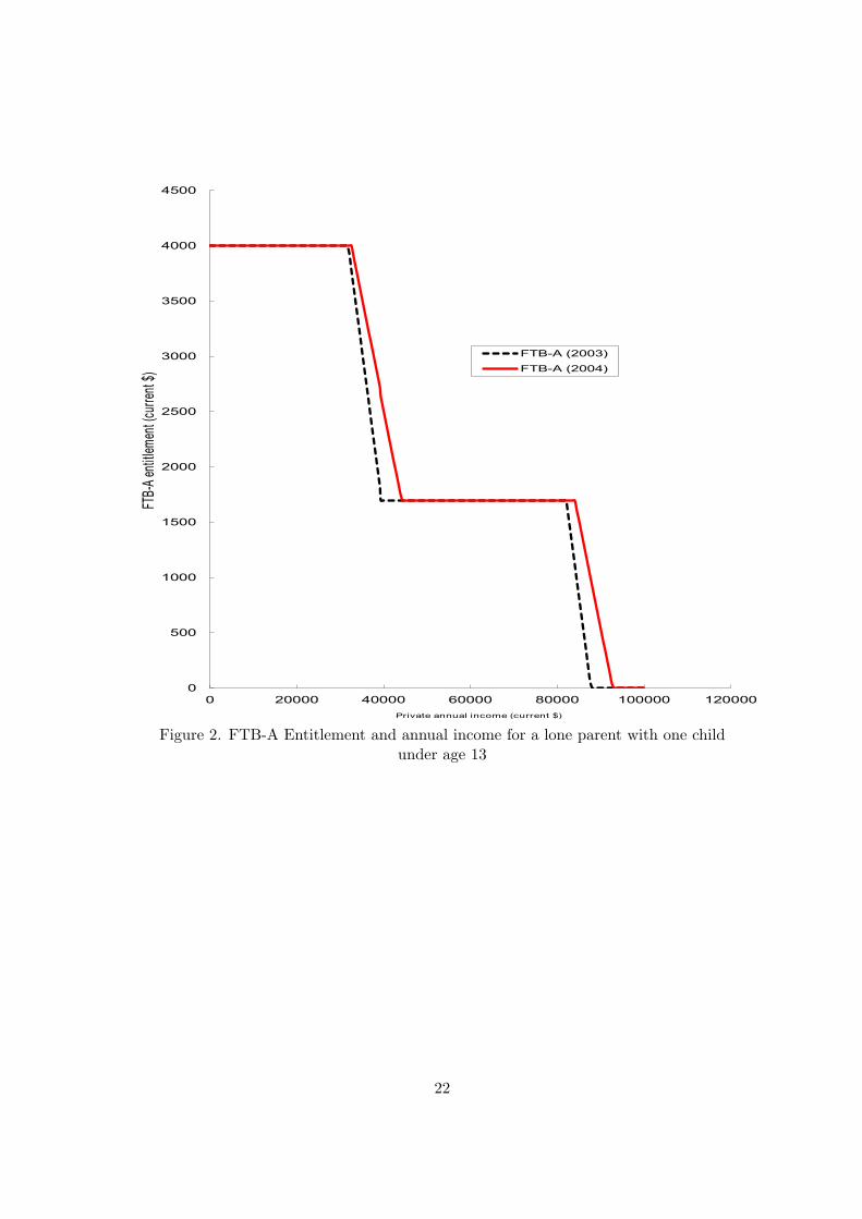
is not means-tested for lone parents.6 FTB-A, on the other hand, depends upon the
age and number of children, and is means-tested. As illustrated by the broken line in
Figure 2, in 2003, a lone parent with one child under 13 could get $4,001.8 of FTB-A
per annum if her annual private income was below $31,755. After that, for each extra
dollar she earns, her FTB-A entitlement was reduced by 30 cents (the ‘taper rate’) until
reaching $1,695 per annum. Her FTB-A entitlement would stay at that level until her
income reached $39,464 before it is again reduced by 30 cents for every additional dollar
earned until reaching an entitlement of zero dollars at an income level of $82,052.7
2.2 Three reforms since 2004
There was one substantial reform introduced in the 2004-05 Financial Year and two
reforms in the 2006-2007 financial year. Our analysis has two parts: the first reform and
the combination of the second and third contemporaneous reforms.
The 2004-2005 reform was part of a legislative package entitled ‘More help for fami-
lies’. The Australian Government lowered the ‘taper rates’ of the means-tests for FTB-A
5All dollar figures in the paper are in Australian dollars. On June 30, 2004, the Australian dollarwas equal to 0.57 Euro or 0.69 U.S. dollar. In June, 2013, the Australian dollar was equal to 0.71 Euroor 0.95 U.S. dollar.
6In 2003, a lone parent received $2,920 per annum if her youngest child was under age 5 and $2,037otherwise.
7Lone parents who qualify for FTB-A also qualify for Rent Assistance if they are renting. Taper ratesfor rent assistance are the same as those for FTB-A because Rent Assistance is treated like a top-up ofthe FTB-A payment.
6
and FTB-B from 30 percent to 20 percent.8 The reform is captured by the movement
from the dotted line to the solid line in Figure 2. This change is equivalent to boosting
the wage of a working lone mother by 10 percent if her annual income is in the tapering
region. If the elasticity of labour supply with respect to own wage is positive, this reform
should lead to an increase in hours worked of lone mothers. The effect of this reform
is even larger for those receiving rent assistance because of its treatment as a top-up to
FTB-A (see footnote 7).
The 2006-2007 reforms consisted of two policy changes. First, PPS eligibility rules
were tightened.9 Under the new rules, new single parent claimants were only eligible for
PPS if their youngest child was under 8 years of age. Previously, single parents were
eligible if their youngest child was under age 16. New income support claimants with
children aged 8 or older no longer qualified for PPS (a pension) but instead could recieve
New Start Allowance–a less generous unemployment benefit which also includes a more
onerous training and job search requirement. Not all single parents were affected as
those on the PPS program prior to the legislative changes were treated under the old
rules provided that their relationship status remained unchanged and that they never
had any payments cancelled. The PPS payments continued to these individuals as
before, however, these individuals also faced a more onerous training and job search
requirement once their youngest child turned 8. Importantly, single parents who were
already working were unaffected by these changes.
The second reform in 2006-2007 was the introduction of the Child Care Tax Rebate
(CCTR). Families of all types were able to claim 30 per cent of out-of-pocket costs (in
excess of CCB payments) for approved child care up to a maximum of $4,000 per child
per annum. Households were able to claim CCTR for two years prior to the reform
back to the 2004-2005 Financial Year when they filed their tax return for the 2005-06
Financial Year (after 1 July 2006). Most households file their tax return between July
and October, thus the first payment only reached families in late 2006. Initially, CCTR
was introduced as a tax offset so only families with a tax liability could benefit. After
8Lone mothers, not subject to means testing for FTB-B, were not affected by this latter change.9This was part of the legislative package ‘Welfare to Work’.
7
the 2006-2007 Financial Year, it was changed into a transfer payment which households
could access even in the absence of a tax liability. The labour market effects of this
reform are ambiguous. Lowering child care costs lowers the costs of working so this may
encourage people to work more. However, there is also an indirect income effect as the
effective decrease in child care costs might result in a lowering of labour supply.
3 Approach
3.1 Identification
We use single, childless women as a comparison group for single mothers and the
‘difference-in-differences’ approach to identify the effects of the policy.10 The first key
identifying assumption of this approach is that single childless women are not affected
by the reforms. Given that we are analyzing administrative rule changes which did
not apply in any way to single, childless women, this assumption would appear to be
met. The second key identifying assumption required is that no other factors affected
the two groups differently over the same period. The period that we analyze was one
of robust economic and job growth in Australia, the benefits of which seemed to be
spread across most demographic groups. We can not find any reason why employment
and hours changes, the variables we analyze, would have been affected differentially for
these two groups apart from the reform. Many other studies use childless women as
a control group for lone mothers (see Eissa and Liebman (1996), Gregg and Harkness
(2003), Francesconi and Klaauw (2007) and Blundell et al. (2008)).11
We present regression estimates in what follows. We check the validity of our re-
gression estimates and the validity of the comparison group in a number of ways. We
compare the characteristics of our treatment and control group; we use nonparametric
matching; and we restrict the sample in various ways all of which are described below in
section 5. Our results are robust to these alternative approaches. In order to avoid the
10For discussions of the approach, see Ashenfelter (1978), Heckman and Robb (1985), Blundell andMaCurdy (1999), Meyer (1995) and Angrist and Kruger (1999).
11Doiron (2004) uses married mothers as a control group. This would be inappropriate in our caseas married mothers were affected by the reforms we analyze such as changes in FTB-B. The legislativereform packages we analyze also had other changes which applied to couple-headed households.
8
confounding effect of changes in labour force status which are caused by the birth of a
child or changes in relationship status, we restrict our estimation sample to those indi-
viduals who are lone mothers in both waves and those who are single, childless women
in both waves. We thus do not analyze any impact which the reforms might have on
fertility or relationship status which are likely to be very small.
One issue for comparability of our treatment and control groups is that the changing
ages of children in the lone mother households across time will have labour supply effects
which the single, childless women will not experience. In order to deal with this, we
control for the changes in the number of children in different age ranges in the household.
The age ranges are chosen to reflect schooling availability and differing care demands
for children of different ages. We also, in the sensitivity tests presented below, restrict
the sample to lone mothers whose children remain in the same age group before and
after the policy change. Our results do not appear to be sensitive to this issue.
We specify three different models to analyse the effect of the reforms: (1) change
in hours worked conditional on working before and after the reforms; (2) the probabil-
ity of being employed conditional on not-working before the reform; (3) unconditional
probability of employment.
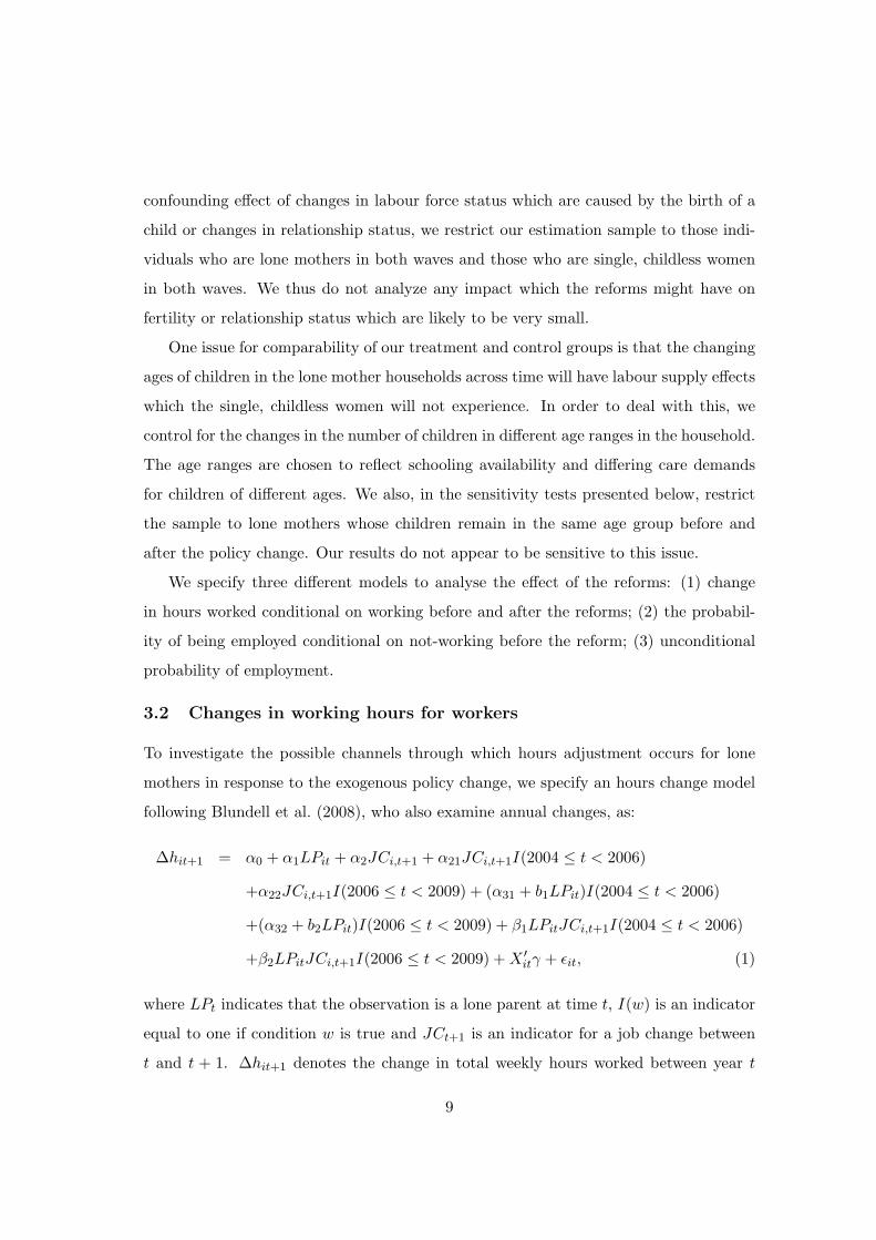
3.2 Changes in working hours for workers
To investigate the possible channels through which hours adjustment occurs for lone
mothers in response to the exogenous policy change, we specify an hours change model
following Blundell et al. (2008), who also examine annual changes, as:
+α22JCi,t+1I(2006 ≤ t < 2009) + (α31 + b1LPit)I(2004 ≤ t < 2006)
+(α32 + b2LPit)I(2006 ≤ t < 2009) + β1LPitJCi,t+1I(2004 ≤ t < 2006)
+β2LPitJCi,t+1I(2006 ≤ t < 2009) +X ′itγ + ϵit, (1)
where LPt indicates that the observation is a lone parent at time t, I(w) is an indicator
equal to one if condition w is true and JCt+1 is an indicator for a job change between
t and t + 1. ∆hit+1 denotes the change in total weekly hours worked between year t
9
and t+ 1; Xit is a vector of observables including levels measured at t and the changes
between t and t + 1; and ϵit captures unobserved impacts on hours changes. I(2004 ≤
t < 2006) and I(2006 ≤ t < 2009) indicate the periods after the 2004 and 2006 reforms,
respectively. Included in Xit are log wage, a quadratic polynomial in age, indicators for
a stated desire to work more (under-employment) or to work less (over-employment),
industry dummies, number and their changes between t and t+1 of children in four age
groups (0 to 5; 6 to 12; 13 to 15; and 16 to 17), type of work contract (casual or fixed
term) and dummies for state/territory and capital city. The variables ‘underemployed’
and ‘over-employed’ are included as indications of the deviation from the individual’s
preferred supply curve. Empirically, they also appear to have strong predictive power
for hours changes. The model is estimated by OLS over nine years of data for all
observations where an individual works in two consecutive years.12
The equation is specified to investigate the role of changing jobs on changing hours
and its interaction with the impact of the reforms. There are two sets of parameters
which capture the effects of the reform. b1 and b2 capture the effects of the two reforms
for workers who stayed in the same job. β1 and β2, meanwhile, capture the additional
effects of the two reforms on workers who changed jobs. If there were no within job
hours restrictions, one would expect β1 = β2 = 0. If this were true, it would indicate
that lone parents could change their hours in response to the reforms by staying in the
same job or by changing jobs in an equal manner. On the other hand, if β1 > 0 (and
similarly for the 2006 reforms), it would indicate a within-job hours restriction.
These four parameters are the difference-in-difference estimators for the two reforms
estimated separately for the group who change jobs and for those who stay in the same
job. As noted by Blundell et al. (2008), equation (1) may suffer from an endogeneity
problem if some omitted factor influences both the job change and the hours change.
However, as they state, it helps to provide an ‘indication of the possible presence of
imperfections or technological rigidities’ in the labour market. By controlling for an
individual’s expressed desire to work more or less we reduce this source of endogeneity.
12We also considered models where we included an interaction term for lone parents and job changes,but this was always insignificant. As there is no reason to believe that the probability of changing jobsdiffers for lone parents in the absence of the reform, we exclude this additional term.
10
Equation (1) is a flexible specification with group-specific discrete jumps after the
reforms for job stayers (α31, α32, b1 and b2) and for job changers (α21, α22, β1 and β2).
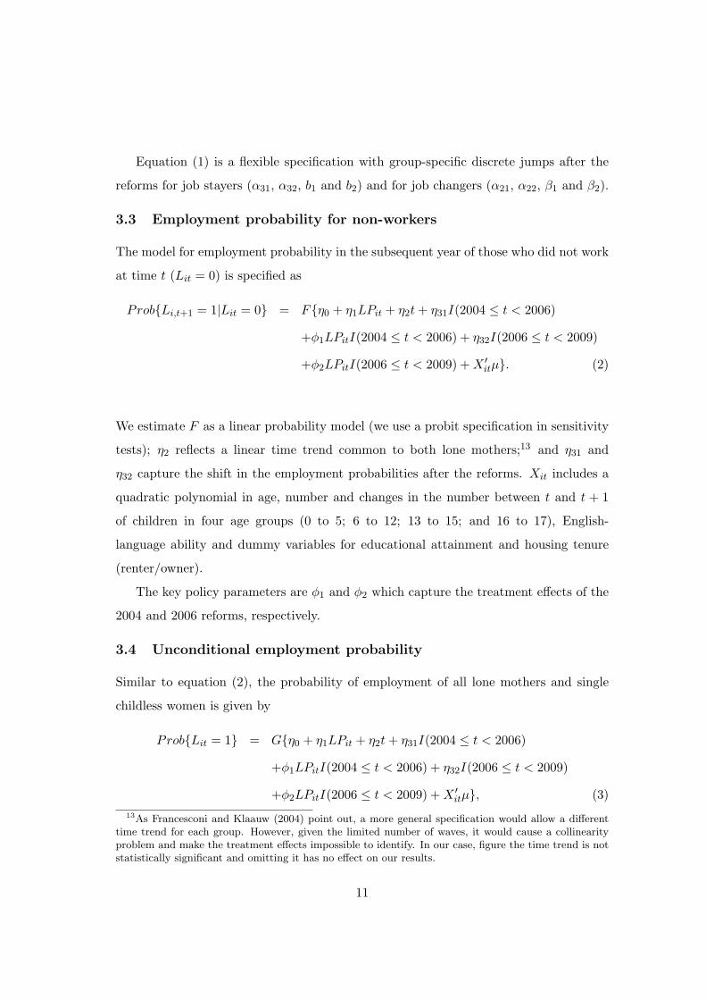
3.3 Employment probability for non-workers
The model for employment probability in the subsequent year of those who did not work
13As Francesconi and Klaauw (2004) point out, a more general specification would allow a differenttime trend for each group. However, given the limited number of waves, it would cause a collinearityproblem and make the treatment effects impossible to identify. In our case, figure the time trend is notstatistically significant and omitting it has no effect on our results.
11
where G is a linear probability function. The difference from equation (2) is that the
dependent variable is contemporaneous with the right-hand side control variables. Xit
contains the same set of control variables as equation (2) with the exception of the
changes in the number of children in different age groups.
4 Data
Data for the analysis are drawn from the first nine waves of the Household Income and
Labour Dynamics in Australia Survey (HILDA) which cover the period 2001 - 2009. The
HILDA Survey is an annual panel survey of Australian households which was begun in
2001.14 There are approximately 7,000 households and 13,000 individuals who respond
in each wave.
We focus on the labour supply of 2,676 lone mothers and single, childless women of
working age (between 15 and 64) excluding those who are students, permanently unable
to work or self-employed. This number also excludes a handful of observations with
missing data on key variables. We are left with 9,239 observations which we use to
analyse the unconditional probability of employment (equation (3)). For the analysis of
hours changes for workers (equation (1)), we restrict the sample to those whose status
as lone parents or single, childless women is unchanged and who are are working for two
consecutive waves. This provides 3,565 observations on 1,214 women. The sample used
to estimate the employment probability conditional on not working in the previous year
(equation (2)) consists of 2,148 observations on 760 women who remain in the same lone
parents/single women status in two consecutive waves and are (not) working in the first
of those two waves.
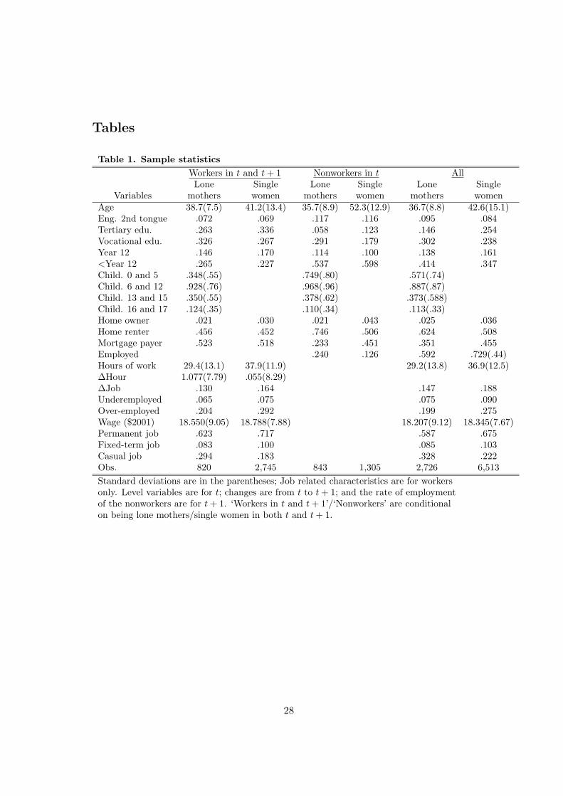
Sample statistics are presented in Table 1. From the table, it can be seen that the
characteristics of lone mothers are different from those of single childless women. How-
ever, if we consider the subset of workers, they are more similar. Overall, as expected,
lone mothers are less educated, younger and more likely to be renters. They are also less
14See Watson and Wooden (2002) for more details.
12
likely to participate in the labour force and, when they do work, work fewer hours. The
biggest difference is between the non-working lone mothers and their single, childless
counterparts. The latter group is much older (with average age of 53 years). This may
invalidate one of our identification requirements. We check this by restricting the age of
the comparison group to 50 or less in one of the sensitivity tests which we conduct and
describe below in section 5.4. The lone parents and single, childless women who work
are more comparable in their characteristics, and they are better educated than the non-
workers. However, their labour supply differs. The lone mothers are more often casual
workers, work fewer hours and are less likely to report being under- or over-employed.
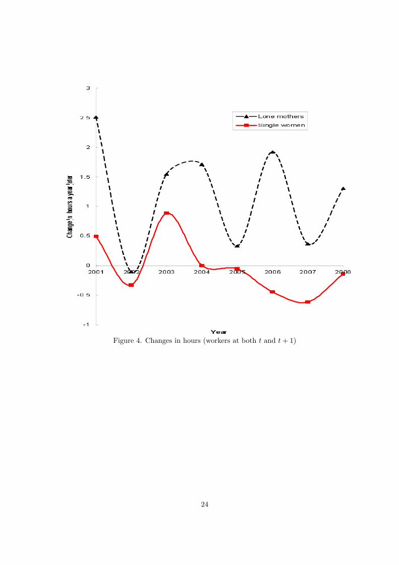
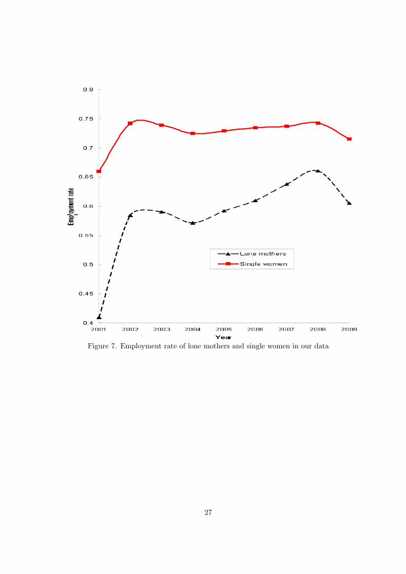
Figures 3 through 7 compare the patterns of labour supply between lone mothers
and single, childless women. From these pictures, we can see that labour supply differs
by group. In Figures 3 and 4, we plot average hours of work and the change of hours
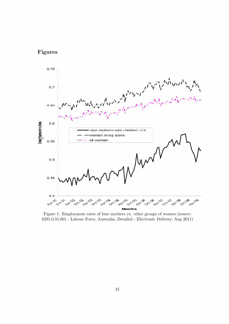
for workers, respectively. Consistent with Figure 1, Figure 3 shows that lone mothers’
hours of work increased in the second half of the last decade but those of single, childless
women remained stable. Figure 4 shows that the change of hours for lone mothers are
positive except in 2002 and are more volatile than the changes in hours of single, childless
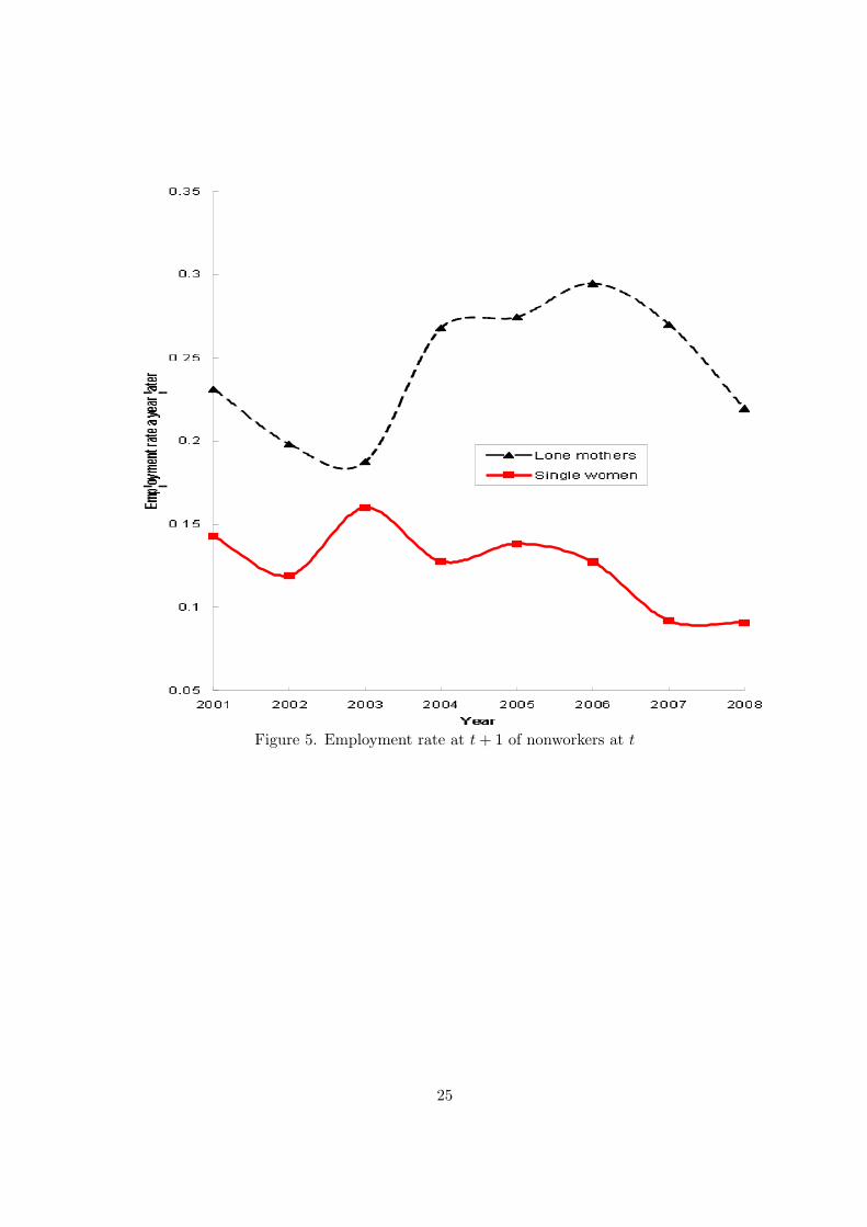
women. Figure 5 shows employment rates conditional on not working in the previous
period. Future employment rates for non-working lone mothers are a bit higher since
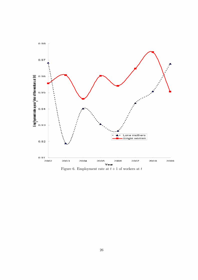
2005 and the pattern is different from that of single, childless women. From Figure 6,
however, we can see that the difference in the patterns of remaining employed for workers
is less pronounced. Figure 7 confirms the overall increase in lone mothers’ employment
across our sample period.
5 Results
We estimate each model for the full sample and also for various sub-samples partitioned
by mother’s education, number of children and age of youngest child, to analyse potential
heterogeneity of policy effects. For the sake of conciseness, we only report the main
parameter estimates. Full regression results are available on request.
13
5.1 Channel of hours adjustment for workers
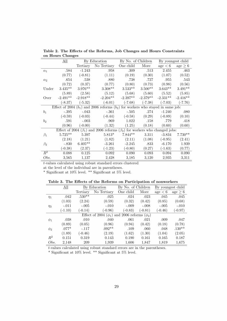
In Table 2, we present the parameter estimates of the treatment effects of the reforms on
lone mothers’ working hours. In the first column we present results from estimation on
the full sample with the remaining columns providing estimates on selected sub-samples
of interest.
For those who stay in their jobs we find no effect of the reforms on working hours–
b1 and b2 are both insignificant. For those that change jobs, we find a positive and
statistically significant effect of the 2004 reform. Working mothers who changed jobs
increased their hours of work by 5.3 hours per week (b1+β1) in response to the reforms.
Looking further across the table, we can see that the effect of the 2004 reform is not
constant across all sub-populations. The effect appears stronger for women with fewer
and older children. These women likely face lower costs to work additional hours.
For the 2006 reforms, we do not find a statistically significant effect of the reforms
when we consider the entire sample. However, we do find a statistically significant effect
on working hours for women with tertiary education of about 7.6 hours per week. This
effect operates through the channel of changing jobs. This seems consistent with the
CCTR reforms of 2006. Even before the reforms, women with tertiary education earn
more and use more child care, CCTR is not means-tested and CCTR is only valuable
when there is a tax liability to be offset. Thus the value of CCTR is higher for these
women.15 The changes to PPS eligibility were not expected to influence working hours
for workers as women who were already working were not impacted by these reforms.
So in the case of changes in working hours for those already working our evaluation of
the 2006 reforms can be considered an evaluation of the introduction of CCTR.
We can also see from Table 2 that a self-reported desire to work more or less hours
is highly predictive of future hour changes. Those who report wanting to work more
increase their work hours by 3.5 hours per week on average relative to those who are
satisfied with their hours whereas those who report wanting to work less decrease their
work hours by 2.5 hours per week on average relative to those who are satisfied with
15This result is consistent with Gong and Breunig (2012) who simulated the ex ante effects of CCTRwith a structural child care and labour supply model.
14
their hours.
Overall, the results provide evidence that there are important within-job hour re-
strictions in the Australian labour market. Changing jobs appears to be an important
channel for all workers to respond to the 2004 policy reforms. It is also the primary
channel by which higher educated workers respond to the 2006 reforms.
5.2 Subsequent Employment of Nonworkers
Table 3 summarises the key parameter estimates from the nonworkers’ subsequent em-
ployment probability equation. The statistical significance of ϕ2 and the insignificant ϕ1
coefficient indicate that the 2006 reforms had a positive effect on the future employment
probability of non-workers but that the 2004 reforms had no effect. This is consistent
with our expectations. The 2006 reforms lowered the cost of working through the intro-
duction of CCTR and also tightened rules and activity tests for receipt of PPS which
had the effect of pushing people into a choice between a lower payment (New Start Al-
lowance) or employment. The combination of these two should have a clear employment
incentive which is particularly concentrated among lone mothers who are less educated
and have older children as can be seen from the other columns of Table 3. The 2004
reform did not have a particularly strong employment incentive for those not already
employed and our insignificant parameter estimate can be interpreted as an indication
that the modest improvements to work incentives were outweighted to a great degree
by fixed costs of working for non-workers.
We also estimated equation (2) for workers (that is, conditional on working at time
t) but omit the results for conciseness. We find no effects of the reforms (ϕ1 and ϕ2
are both statistically insignificant) which is consistent with our expectation that neither
reform should lead to a shift in employment probability for those already employed.
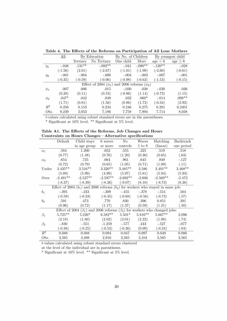
5.3 Employment of All Lone Mothers
In addition to analyzing employment effects conditional on previous employment status,
we estimated the unconditional employment probability for all lone mothers and single
childless women (equation (3)). The key parameters are presented in Table 4. The
15
estimates of ϕ1 and ϕ2 confirm the findings in section 5.2: while the 2004 reform did
not have any employment effects, the 2006 reforms brought about an increase in the
employment of lone mothers with lower education and fewer and older children.
5.4 Sensitivity Tests
To check the specification, the functional form, the validity of the common support
assumption and the potential impact of other factors, we conducted a range of sensitivity
tests for each of the estimated equations. First of all, for the two conditional equations,
although we controlled both the level and the change in the number of children in each
age group, aging of the children could still confound the estimated treatment effect as
discussed above. To further reduce the impact of children’s aging (although we can
never completely remove it), we further restrict the sample to observations where the
youngest child remains in the same age group at t and t+1. Secondly, to check whether
there is a problem caused by non-random attrition, we restrict the sample to individuals
who were observed in at least 6 waves. Thirdly, we estimate the model excluding the
ninth wave. Because CCTR changed (it was increased from 30 to 50 percent as of July
2008) and the on-set of the Global Financial Crisis may have affected our two groups
differently (although we think this is unlikely), the ninth wave may be quite different
from other waves.
In addition, including many covariates in the models may make it harder to find
over-lapping groups with the same characteristics in both the treatment and control
groups. In the treatment literature this is called the common support problem. To
see whether this affects our results, we combine the difference-in-difference estimator
with propensity score matching. We re-estimated equations (2) and (3) with local linear
regression matching (see for example, Heckman, Ichimura and Todd (1997) and Fan
(1992)). For equation (1), we used linear regression matching as the number of observa-
tions in each cell is too small to undertake a non-parametric approach. Equation (2) was
also estimated with the comparison group restricted to be 50 years of age or younger as
discussed above. All equations are also estimated without controls, and where possible,
using a probit functional form. Lastly, a natural way to check the condition that the
16
untreated response changes are the same across the treatment and control groups is to
backtrack one period and examine the response changes in two pre-treatment periods.
If the condition does not hold in the pre-treatment periods, then a pre-treatment gap
may exist.
The key results of these sensitivity tests are summarised in Tables A1, A2 and A3,
respectively. By and large, these results show that the estimates of the benchmark
model (the first column of each table) are robust. In particular, the last column in each
table shows that pre-treatment gaps do not exist so the assumption that the untreated
response changes are the same across the treatment and control groups appears to hold.
6 Conclusions
The classical labour supply model predicts that changed welfare rules will alter women’s
optimal labour supply. Preferred hours will change for those who are working and the
decision to participate for workers and non-workers will also be affected. That model
assumes that workers can adjust hours of work at will within their present employment
relationships.
Our paper illustrates the relationship between different policy designs and heteroge-
nous labour supply outcomes for lone mothers. We find that two reforms which changed
the work incentives for lone mothers in Australia increased working hours of those who
were working and employment of non-workers, but that they had no effect on the con-
tinued probability of remaining in employment for workers. The adjustment in working
hours was largely through changing employers in an environment where working hours
are often constrained within jobs. The 2004 reform had positive effects on hours of work
by working lone mothers, but only through job changes. The effects were concentrated
among lone mothers with lower education and with fewer and older children. The 2006
reforms contributed to an increased probability of employment in subsequent periods for
those who were not working pre-reform. Again, effects were concentrated among lone
mothers with lower education and with fewer and older children. The 2006 reforms also
increased hours of work for higher educated lone mothers who were already employed.
Again, working hours changes occurred through the channel of changing employers.
17
These results highlight some caveats to the standard model. First, in-work rigidities
appear to exist. The ability of policy changes to induce working hour changes therefore
may be enhanced or diminished by the degree of dynamism in the labour market. Second,
some reforms seem to have no effect on participation. This is consistent with important
fixed costs of working which should be accounted for when modeling labour supply.
Third, tightened welfare rules appear to have larger effects on those with lower education
whereas increased child care tax rebates have a larger impact on those with higher
education. This is consistent with the higher incomes of those with more education and
the nature of the child care subsidy which is delivered through a tax rebate.
References
Altonji, J. G. and Paxson, C. H. (1988). Labour supply preferences, hours constraint,and hours-wage tradeoffs, Journal of Labor Economics 6(2): 254–276.
Altonji, J. G. and Paxson, C. H. (1992). Labour supply, hours constraint, and jobmobility, Journal of Human Resources 27(2): 256–278.
Angrist, J. and Kruger, A. (1999). Empirical stragegies in labor economics, in O. Ashen-felter and D. Card (eds), Handbook of Labor Economics, Vol. 3A, Amsterdam: ElsevierScience, chapter 23, pp. 1277–1366.
Ashenfelter, O. C. (1978). Estimating the effect of training programs on earnings, Reviewof Economics and Statistics 60(1): 47–57.
Blundell, R., Brewer, M. and Francesconi, M. (2008). Job changes and hours changes:Understanding the path of labor supply adjustment, Journal of Labor Economics26(3): 421–453.
Blundell, R., Brewer, M. and Shephard, A. (2005). Evaluating the labour market impactof working families’ tax credit using difference-in-differences. Open Access publicationsfrom University College London http://discovery.ucl.ac.uk, University CollegeLondon.
Blundell, R. and MaCurdy, T. E. (1999). Labour supply: A review of alternativeapproaches, in O. Arshenfelter and D. Card (eds), Handbook of Labor Economics,Vol. 3A, Amsterdam: Elsevier Science, chapter 27, pp. 1559–1695.
Brewer, M., Duncan, A., Shephard, A. and Suarez, M. J. (2006). Did working families’tax credit work? the impact of in-work support on labour supply in great britain,Labour Economics 13(6): 699–720.
18
Card, D. and Robins, P. K. (1998). Do financial incentives encourage welfare recipientsto work?, Research in Labor Economics 17: 1–56.
Doiron, D. J. (2004). Welfare reform and the labour supply of lone parents in Australia:A natural experiment approach, The Economic Record 80(249): 157–176.
Eissa, N. and Hoynes, H. (2004). Taxes and the labor market participation of marriedcouples: The earned income tax credit”, Journal of Public Economics 88(9-10): 1931–1958.
Eissa, N. and Liebman, J. B. (1996). Labor supply response to the earned income taxcredit, The Quarterly Journal of Economics 112(2): 605–637.
Ellwood, D. T. (2000). The impact of the earned income tax credit and social policy re-forms on work, marriage, and living arrangements, National Tax Journal 53(4): 1063–1106.
Euwals, R. (2001). Female labour supply, flexibility of working hours, and job mobility,Economic Journal 111: C120–C134.
Fan, J. (1992). Design-adaptive nonparametric regression, Journal of the AmericanStatistical Association 87(420): 998–1004.
Francesconi, M. and Klaauw, W. V. D. (2004). The consequences of “in-work” benefitreform in Britian: New evidence from paneld data. ISER Working Paper number2004-13. Colchester: University of Essex, August.
Francesconi, M. and Klaauw, W. V. D. (2007). The socioeconomic consequences of ”in-work” benefit reform for British lone mothers, Journal of Human Resources 42(1): 1–31.
Gong, X. and Breunig, R. (2012). Child Care Assistance: Are Subsidies or Tax CreditsBetter? IZA discussion paper number 6606. Available from http://ftp.iza.org/
dp6606.pdf.
Gregg, P. and Harkness, S. (2003). Welfare reform and lone parents employment in theUK. CMPO Working paper series, No. 03/072, Department of Economics, Universityof Bristol.
Ham, J. C. (1982). Estimation of a labour supply model with censoring due to unem-ployment and underemployment, Review of Economic Studies 49(3): 335–354.
Heckman, J. J., Ichimura, H. and Todd, P. E. (1997). Matching as an econometricevaluation estimator: Evidence from evaluating a job training programme, The Reviewof Economic Studies 64(4): 605–654.
Heckman, J. J. and Robb, R. (1985). Alternative methods for evaluating the impact ofinterventions, in J. J. Heckman and B. S. Singer (eds), Longitudinal Analysis of LaborMarket Data, Cambridge, UK: Cambridge University Press, pp. 146–245. EconometricSociety Monograph Series number 10.
19
Hotz, J. V. and Scholz, J. K. (2003). The earned income tax credit, in R. A. Moffitt(ed.), Means-tested Transfer Programs in the United States, Chicago: University ofChicago Press.
Hotz, V. J., Mullin, C. H. and Scholz, J. K. (2002). Welfare, employment, and income:Evidence on the effects of benefit reductions from california, American EconomicReview 92(2): 380–384.
Leigh, A. K. (2005). Optimal design of earned income tax credits: Evidence froma british natural experiment. CEPR Discussion Papers 488, Centre for EconomicPolicy Research, Research School of Economics, Australian National University.
Lundberg, S. (1985). Tied wage-hours offers and the endogeneity of wages, Review ofEconomics and Statistics 67(2): 405–410.
Meyer, B. D. (1995). Natural and quasi-experiments in economics, Journal of Buinessand Economic Statstics 13(2): 151–161.
Moffitt, R. A. (1984). The estimation of a joint wage-hours labor supply model, Journalof Labor Economics 2(4): 550–566.
Stewart, M. B. and Swaffield, J. K. (1997). Constraints on the desired hours of work ofBritish men, Economic Journal 107(441): 520–535.
20
Figures
Figure 1. Employment rates of lone mothers vs. other groups of women (source:6291.0.55.001 - Labour Force, Australia, Detailed - Electronic Delivery, Aug 2011)
21
0
500
1000
1500
2000
2500
3000
3500
4000
4500
0 20000 40000 60000 80000 100000 120000
FTB-
A en
title
men
t (cu
rrent
$)
Private annual income (current $)
FTB-A (2003)
FTB-A (2004)
Figure 2. FTB-A Entitlement and annual income for a lone parent with one childunder age 13
22
Figure 3. Hours of work (workers at both t and t+ 1)
23
Figure 4. Changes in hours (workers at both t and t+ 1)
24
Figure 5. Employment rate at t+ 1 of nonworkers at t
25
Figure 6. Employment rate at t+ 1 of workers at t
26
Figure 7. Employment rate of lone mothers and single women in our data
27
Tables
Table 1. Sample statistics
Workers in t and t+ 1 Nonworkers in t AllLone Single Lone Single Lone Single
Standard deviations are in the parentheses; Job related characteristics are for workersonly. Level variables are for t; changes are from t to t+ 1; and the rate of employmentof the nonworkers are for t+ 1. ‘Workers in t and t+ 1’/‘Nonworkers’ are conditionalon being lone mothers/single women in both t and t+ 1.
28
Table 2. The Effects of the Reforms, Job Changes and Hours Constraintson Hours Changes
All By Education By No. of Children By youngest childTertiary No Tertiary One child More age < 6 age ≥ 6
t-values calculated using robust standard errors clusteredat the level of the individual are in parentheses.* Significant at 10% level. ** Significant at 5% level.
Table 3. The Effects of the Reforms on Participation of nonworkers
All By Education By No. of Children By youngest childTertiary No Tertiary One child More age < 6 age ≥ 6
t-values calculated using robust standard errors clusteredat the level of the individual are in parentheses.* Significant at 10% level. ** Significant at 5% level.
30
Table A2. The Effects of the Reforms on Participation ofnonworkers—-Alternative specifications
Default Child same 6 waves No Probit Waves Compare Non-par. Backtrackage group or more controls 1 to 8 Age≤50 matching† one period
t-values calculated using robust standard errors are in the parentheses.* Significant at 10% level. ** Significant at 5% level. # Pseudo R2.†Local linear regression matching with standard errors bootstrapped with 500 replications.
Table A3. The Effects of the Reforms on Participation ofLone mothers—-Alternative specifications
Default Observed in No other Probit Waves Non-par. Backtrack> 5 waves controls 1 to 8 matching† one period
t-values calculated using robust standard errors are in the parentheses.* Significant at 10% level. ** Significant at 5% level. # Pseudo R2.†Local linear regression matching with standard errors bootstrappedwith 500 replications.