Large Kernel Matters ——Improve Semantic Segmentation by Global Convolutional Network

Chao Peng Xiangyu Zhang Gang Yu Guiming Luo Jian SunSchool of Software, Tsinghua University, {pengc14@mails.tsinghua.edu.cn, gluo@tsinghua.edu.cn}

Megvii Inc. (Face++), {zhangxiangyu, yugang, sunjian}@megvii.com

Abstract

One of recent trends [30, 31, 14] in network architec-ture design is stacking small filters (e.g., 1x1 or 3x3) in theentire network because the stacked small filters is more ef-ficient than a large kernel, given the same computationalcomplexity. However, in the field of semantic segmenta-tion, where we need to perform dense per-pixel prediction,we find that the large kernel (and effective receptive field)plays an important role when we have to perform the clas-sification and localization tasks simultaneously. Followingour design principle, we propose a Global ConvolutionalNetwork to address both the classification and localizationissues for the semantic segmentation. We also suggest aresidual-based boundary refinement to further refine the ob-ject boundaries. Our approach achieves state-of-art perfor-mance on two public benchmarks and significantly outper-forms previous results, 82.2% (vs 80.2%) on PASCAL VOC2012 dataset and 76.9% (vs 71.8%) on Cityscapes dataset.

1. Introduction

Semantic segmentation can be considered as a per-pixelclassification problem. There are two challenges in thistask: 1) classification: an object associated to a specific se-mantic concept should be marked correctly; 2) localization:the classification label for a pixel must be aligned to the ap-propriate coordinates in output score map. A well-designedsegmentation model should deal with the two issues simul-taneously.

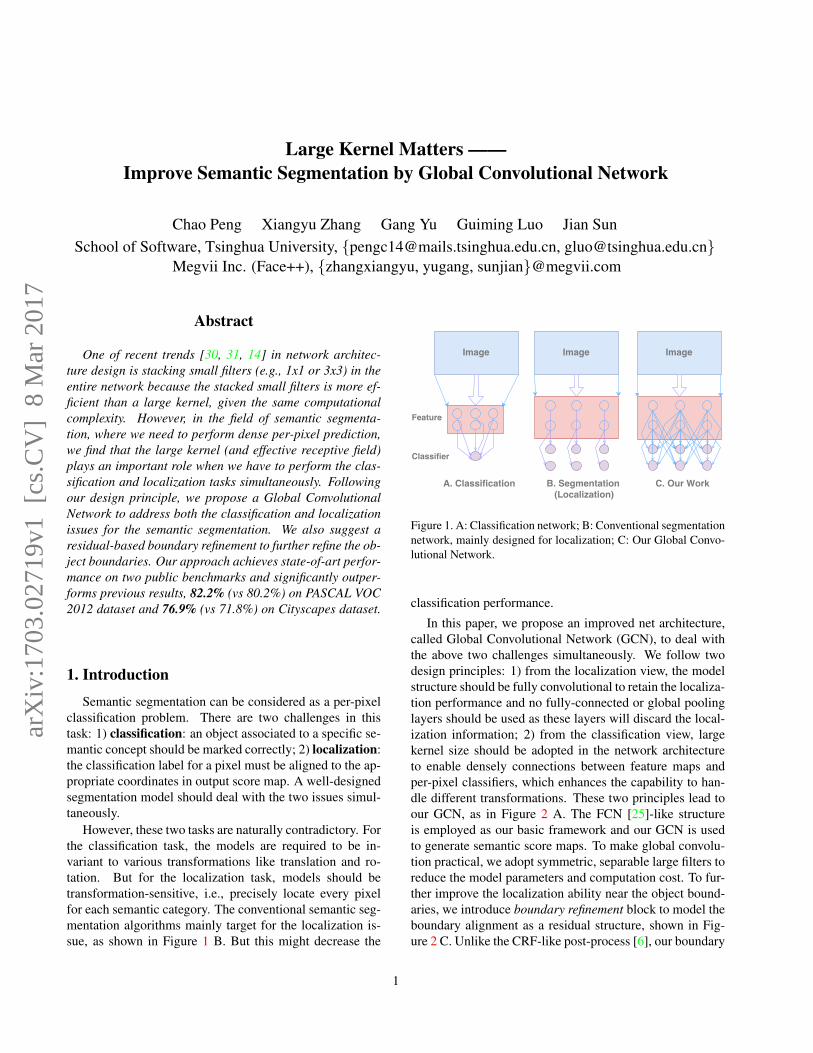
However, these two tasks are naturally contradictory. Forthe classification task, the models are required to be in-variant to various transformations like translation and ro-tation. But for the localization task, models should betransformation-sensitive, i.e., precisely locate every pixelfor each semantic category. The conventional semantic seg-mentation algorithms mainly target for the localization is-sue, as shown in Figure 1 B. But this might decrease the

Figure 1. A: Classification network; B: Conventional segmentationnetwork, mainly designed for localization; C: Our Global Convo-lutional Network.

classification performance.

In this paper, we propose an improved net architecture,called Global Convolutional Network (GCN), to deal withthe above two challenges simultaneously. We follow twodesign principles: 1) from the localization view, the modelstructure should be fully convolutional to retain the localiza-tion performance and no fully-connected or global poolinglayers should be used as these layers will discard the local-ization information; 2) from the classification view, largekernel size should be adopted in the network architectureto enable densely connections between feature maps andper-pixel classifiers, which enhances the capability to han-dle different transformations. These two principles lead toour GCN, as in Figure 2 A. The FCN [25]-like structureis employed as our basic framework and our GCN is usedto generate semantic score maps. To make global convolu-tion practical, we adopt symmetric, separable large filters toreduce the model parameters and computation cost. To fur-ther improve the localization ability near the object bound-aries, we introduce boundary refinement block to model theboundary alignment as a residual structure, shown in Fig-ure 2 C. Unlike the CRF-like post-process [6], our boundary

1

arX

iv:1

703.

0271

9v1

[cs

.CV

] 8

Mar

201

7

refinement block is integrated into the network and trainedend-to-end.

Our contributions are summarized as follows: 1) we pro-pose Global Convolutional Network for semantic segmen-tation which explicitly address the “classification” and “lo-calization” problems simultaneously; 2) a Boundary Refine-ment block is introduced which can further improve the lo-calization performance near the object boundaries; 3) weachieve state-of-art results on two standard benchmarks,with 82.2% on PASCAL VOC 2012 and 76.9% on theCityscapes.

2. Related WorkIn this section we quickly review the literatures on se-

mantic segmentation. One of the most popular CNN basedwork is the Fully Convolutional Network (FCN) [25]. Byconverting the fully-connected layers into convolutionallayers and concatenating the intermediate score maps, FCNhas outperformed a lot of traditional methods on semanticsegmentation. Following the structure of FCN, there areseveral works trying to improve the semantic segmentationtask based on the following three aspects.

Context Embedding in semantic segmentation is a hottopic. Among the first, Zoom-out [26] proposes a hand-crafted hierarchical context features, while ParseNet [23]adds a global pooling branch to extract context information.Further, Dilated-Net [36] appends several layers after thescore map to embed the multi-scale context, and Deeplab-V2 [7] uses the Atrous Spatial Pyramid Pooling, which is acombination of convolutions, to embed the context directlyfrom feature map.

Resolution Enlarging is another research direction insemantic segmentation. Initially, FCN [25] proposes thedeconvolution (i.e. inverse of convolution) operation to in-crease the resolution of small score map. Further, Deconv-Net [27] and SegNet [3] introduce the unpooling operation(i.e. inverse of pooling) and a glass-like network to learnthe upsampling process. More recently, LRR [12] arguesthat upsampling a feature map is better than score map. In-stead of learning the upsampling process, Deeplab [24] andDilated-Net [36] propose a special dilated convolution todirectly increase the spatial size of small feature maps, re-sulting in a larger score map.

Boundary Alignment tries to refine the predictions nearthe object boundaries. Among the many methods, Condi-tional Random Field (CRF) is often employed here becauseof its good mathematical formation. Deeplab [6] directlyemploys denseCRF [18], which is a CRF-variant built onfully-connected graph, as a post-processing method afterCNN. Then CRFAsRNN [37] models the denseCRF intoa RNN-style operator and proposes an end-to-end pipeline,yet it involves too much CPU computation on Permutohe-dral Lattice [1]. DPN [24] makes a different approxima-

tion on denseCRF and put the whole pipeline completely onGPU. Furthermore, Adelaide [21] deeply incorporates CRFand CNN where hand-crafted potentials is replaced by con-volutions and nonlinearities. Besides, there are also somealternatives to CRF. [4] presents a similar model to CRF,called Bilateral Solver, yet achieves 10x speed and com-parable performance. [16] introduces the bilateral filter tolearn the specific pairwise potentials within CNN.

In contrary to previous works, we argues that semanticsegmentation is a classification task on large feature mapand our Global Convolutional Network could simultane-ously fulfill the demands of classification and localization.

3. ApproachIn this section, we first propose a novel Global Convolu-

tional Network (GCN) to address the contradictory aspects— classification and localization in semantic segmentation.Then using GCN we design a fully-convolutional frame-work for semantic segmentation task.

3.1. Global Convolutional Network

The task of semantic segmentation, or pixel-wise classi-fication, requires to output a score map assigning each pixelfrom the input image with semantic label. As mentioned inIntroduction section, this task implies two challenges: clas-sification and localization. However, we find that the re-quirements of classification and localization problems arenaturally contradictory: (1) For classification task, modelsare required invariant to transformation on the inputs — ob-jects may be shifted, rotated or rescaled but the classifica-tion results are expected to be unchanged. (2) While for lo-calization task, models should be transformation-sensitivebecause the localization results depend on the positions ofinputs.

In deep learning, the differences between classificationand localization lead to different styles of models. For clas-sification, most modern frameworks such as AlexNet [20],VGG Net [30], GoogleNet [31, 32] or ResNet [14] em-ploy the ”Cone-shaped” networks shown in Figure 1 A:features are extracted from a relatively small hidden layer,which is coarse on spatial dimensions, and classifiersare densely connected to entire feature map via fully-connected layer [20, 30] or global pooling layer [31, 32, 14],which makes features robust to locally disturbances and al-lows classifiers to handle different types of input transfor-mations. For localization, in contrast, we need relativelylarge feature maps to encode more spatial information. Thatis why most semantic segmentation frameworks, such asFCN [25, 29], DeepLab [6, 7], Deconv-Net [27], adopt”Barrel-shaped” networks shown in Figure 1 B. Techniquessuch as Deconvolution [25], Unpooling [27, 3] and Dilated-Convolution [6, 36] are used to generate high-resolutionfeature maps, then classifiers are connected locally to each

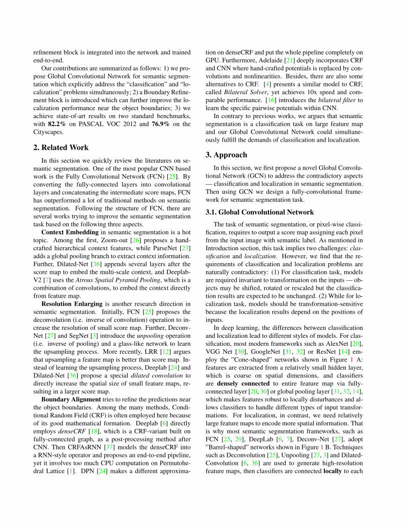
Figure 2. An overview of the whole pipeline in (A). The details of Global Convolutional Network (GCN) and Boundary Refinement (BR)block are illustrated in (B) and (C), respectively.

spatial location on the feature map to generate pixel-wisesemantic labels.

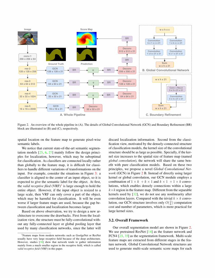
We notice that current state-of-the-art semantic segmen-tation models [25, 6, 27] mainly follow the design princi-ples for localization, however, which may be suboptimalfor classification. As classifiers are connected locally ratherthan globally to the feature map, it is difficult for classi-fiers to handle different variations of transformations on theinput. For example, consider the situations in Figure 3: aclassifier is aligned to the center of an input object, so it isexpected to give the semantic label for the object. At first,the valid receptive filed (VRF)1 is large enough to hold theentire object. However, if the input object is resized to alarge scale, then VRF can only cover a part of the object,which may be harmful for classification. It will be evenworse if larger feature maps are used, because the gap be-tween classification and localization becomes larger.

Based on above observation, we try to design a new ar-chitecture to overcome the drawbacks. First from the local-ization view, the structure must be fully-convolutional with-out any fully-connected layer or global pooling layer thatused by many classification networks, since the latter will

1Feature maps from modern networks such as GoolgeNet or ResNetusually have very large receptive field because of the deep architecture.However, studies [38] show that network tends to gather informationmainly from a much smaller region in the receptive field, which is calledvalid receptive field (VRF) in this paper.

discard localization information. Second from the classi-fication view, motivated by the densely-connected structureof classification models, the kernel size of the convolutionalstructure should be as large as possible. Specially, if the ker-nel size increases to the spatial size of feature map (namedglobal convolution), the network will share the same ben-efit with pure classification models. Based on these twoprinciples, we propose a novel Global Convolutional Net-work (GCN) in Figure 2 B. Instead of directly using largerkernel or global convolution, our GCN module employs acombination of 1 × k + k × 1 and k × 1 + 1 × k convo-lutions, which enables densely connections within a largek×k region in the feature map. Different from the separablekernels used by [32], we do not use any nonlinearity afterconvolution layers. Compared with the trivial k × k convo-lution, our GCN structure involves only O( 2k ) computationcost and number of parameters, which is more practical forlarge kernel sizes.

3.2. Overall Framework

Our overall segmentation model are shown in Figure 2.We use pretrained ResNet [14] as the feature network andFCN4 [25, 35] as the segmentation framework. Multi-scalefeature maps are extracted from different stages in the fea-ture network. Global Convolutional Network structures areused to generate multi-scale semantic score maps for each

Figure 3. Visualization of valid receptive field (VRF) introduced by [38]. Regions on images show the VRF for the score map located atthe center of the bird. For traditional segmentation model, even though the receptive field is as large as the input image, however, the VRFjust covers the bird (A) and fails to hold the entire object if the input resized to a larger scale (B). As a comparison, our Global ConvolutionNetwork significantly enlarges the VRF (C).

class. Similar to [25, 35], score maps of lower resolutionwill be upsampled with a deconvolution layer, then addedup with higher ones to generate new score maps. The finalsemantic score map will be generated after the last upsam-pling, which is used to output the prediction results.

In addition, we propose a Boundary Refinement (BR)block shown in Figure 2 C. Here, we models the boundaryalignment as a residual structure. More specifically, we de-fine S as the refined score map: S = S +R(S), where S isthe coarse score map and R(·) is the residual branch. Thedetails can be referred to Figure 2.

4. ExperimentWe evaluate our approach on the standard benchmark

PASCAL VOC 2012 [11, 10] and Cityscapes [8]. PAS-CAL VOC 2012 has 1464 images for training, 1449 imagesfor validation and 1456 images for testing, which belongsto 20 object classes along with one background class. Wealso use the Semantic Boundaries Dataset [13] as auxiliarydataset, resulting in 10,582 images for training. We choosethe state-of-the-art network ResNet 152 [14] (pretrained onImageNet [28]) as our base model for fine tuning. Dur-ing the training time, we use standard SGD [20] with batchsize 1, momentum 0.99 and weight decay 0.0005 . Dataaugmentations like mean subtraction and horizontal flip arealso applied in training. The performance is measured bystandard mean intersection-over-union (IoU). All the exper-iments are running with Caffe [17] tool.

In the next subsections, first we will perform a series ofablation experiments to evaluate the effectiveness of our ap-proach. Then we will report the full results on PASCALVOC 2012 and Cityscapes.

4.1. Ablation Experiments

In this subsection, we will make apple-to-apple compar-isons to evaluate our approaches proposed in Section 3. As

mentioned above, we use PASCAL VOC 2012 validationset for the evaluation. For all succeeding experiments, wepad each input image into 512 × 512 so that the top-mostfeature map is 16× 16.

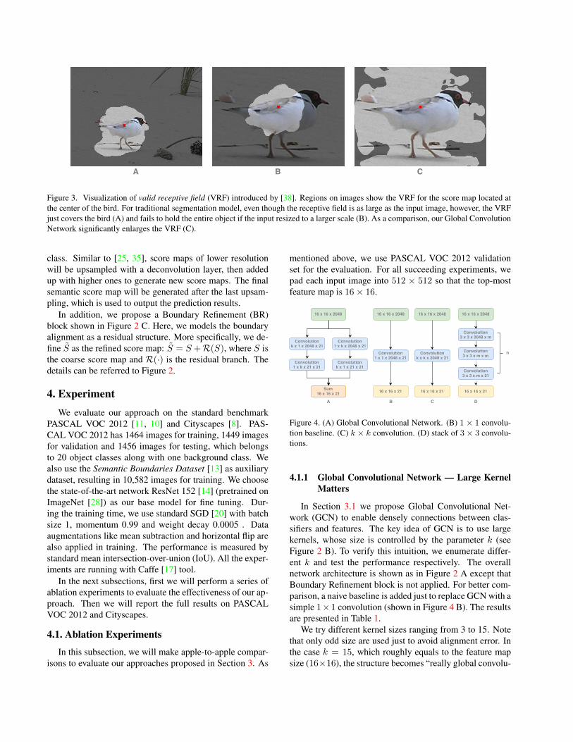
Figure 4. (A) Global Convolutional Network. (B) 1 × 1 convolu-tion baseline. (C) k × k convolution. (D) stack of 3× 3 convolu-tions.

4.1.1 Global Convolutional Network — Large KernelMatters

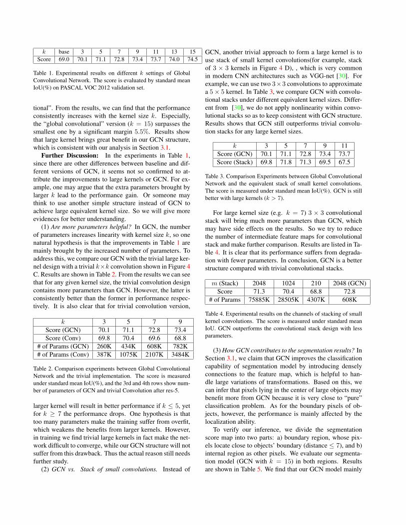
In Section 3.1 we propose Global Convolutional Net-work (GCN) to enable densely connections between clas-sifiers and features. The key idea of GCN is to use largekernels, whose size is controlled by the parameter k (seeFigure 2 B). To verify this intuition, we enumerate differ-ent k and test the performance respectively. The overallnetwork architecture is shown as in Figure 2 A except thatBoundary Refinement block is not applied. For better com-parison, a naive baseline is added just to replace GCN with asimple 1×1 convolution (shown in Figure 4 B). The resultsare presented in Table 1.

We try different kernel sizes ranging from 3 to 15. Notethat only odd size are used just to avoid alignment error. Inthe case k = 15, which roughly equals to the feature mapsize (16×16), the structure becomes “really global convolu-

k base 3 5 7 9 11 13 15Score 69.0 70.1 71.1 72.8 73.4 73.7 74.0 74.5

Table 1. Experimental results on different k settings of GlobalConvolutional Network. The score is evaluated by standard meanIoU(%) on PASCAL VOC 2012 validation set.

tional”. From the results, we can find that the performanceconsistently increases with the kernel size k. Especially,the “global convolutional” version (k = 15) surpasses thesmallest one by a significant margin 5.5%. Results showthat large kernel brings great benefit in our GCN structure,which is consistent with our analysis in Section 3.1.

Further Discussion: In the experiments in Table 1,since there are other differences between baseline and dif-ferent versions of GCN, it seems not so confirmed to at-tribute the improvements to large kernels or GCN. For ex-ample, one may argue that the extra parameters brought bylarger k lead to the performance gain. Or someone maythink to use another simple structure instead of GCN toachieve large equivalent kernel size. So we will give moreevidences for better understanding.

(1) Are more parameters helpful? In GCN, the numberof parameters increases linearity with kernel size k, so onenatural hypothesis is that the improvements in Table 1 aremainly brought by the increased number of parameters. Toaddress this, we compare our GCN with the trivial large ker-nel design with a trivial k×k convolution shown in Figure 4C. Results are shown in Table 2. From the results we can seethat for any given kernel size, the trivial convolution designcontains more parameters than GCN. However, the latter isconsistently better than the former in performance respec-tively. It is also clear that for trivial convolution version,

k 3 5 7 9Score (GCN) 70.1 71.1 72.8 73.4Score (Conv) 69.8 70.4 69.6 68.8

# of Params (GCN) 260K 434K 608K 782K# of Params (Conv) 387K 1075K 2107K 3484K

Table 2. Comparison experiments between Global ConvolutionalNetwork and the trivial implementation. The score is measuredunder standard mean IoU(%), and the 3rd and 4th rows show num-ber of parameters of GCN and trivial Convolution after res-5.

larger kernel will result in better performance if k ≤ 5, yetfor k ≥ 7 the performance drops. One hypothesis is thattoo many parameters make the training suffer from overfit,which weakens the benefits from larger kernels. However,in training we find trivial large kernels in fact make the net-work difficult to converge, while our GCN structure will notsuffer from this drawback. Thus the actual reason still needsfurther study.

(2) GCN vs. Stack of small convolutions. Instead of

GCN, another trivial approach to form a large kernel is touse stack of small kernel convolutions(for example, stackof 3 × 3 kernels in Figure 4 D), , which is very commonin modern CNN architectures such as VGG-net [30]. Forexample, we can use two 3×3 convolutions to approximatea 5× 5 kernel. In Table 3, we compare GCN with convolu-tional stacks under different equivalent kernel sizes. Differ-ent from [30], we do not apply nonlinearity within convo-lutional stacks so as to keep consistent with GCN structure.Results shows that GCN still outperforms trivial convolu-tion stacks for any large kernel sizes.

k 3 5 7 9 11Score (GCN) 70.1 71.1 72.8 73.4 73.7Score (Stack) 69.8 71.8 71.3 69.5 67.5

Table 3. Comparison Experiments between Global ConvolutionalNetwork and the equivalent stack of small kernel convolutions.The score is measured under standard mean IoU(%). GCN is stillbetter with large kernels (k > 7).

For large kernel size (e.g. k = 7) 3 × 3 convolutionalstack will bring much more parameters than GCN, whichmay have side effects on the results. So we try to reducethe number of intermediate feature maps for convolutionalstack and make further comparison. Results are listed in Ta-ble 4. It is clear that its performance suffers from degrada-tion with fewer parameters. In conclusion, GCN is a betterstructure compared with trivial convolutional stacks.

m (Stack) 2048 1024 210 2048 (GCN)Score 71.3 70.4 68.8 72.8

# of Params 75885K 28505K 4307K 608K

Table 4. Experimental results on the channels of stacking of smallkernel convolutions. The score is measured under standard meanIoU. GCN outperforms the convolutional stack design with lessparameters.

(3) How GCN contributes to the segmentation results? InSection 3.1, we claim that GCN improves the classificationcapability of segmentation model by introducing denselyconnections to the feature map, which is helpful to han-dle large variations of transformations. Based on this, wecan infer that pixels lying in the center of large objects maybenefit more from GCN because it is very close to “pure”classification problem. As for the boundary pixels of ob-jects, however, the performance is mainly affected by thelocalization ability.

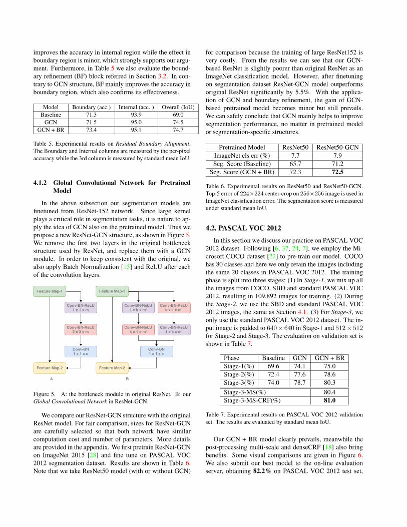
To verify our inference, we divide the segmentationscore map into two parts: a) boundary region, whose pix-els locate close to objects’ boundary (distance ≤ 7), and b)internal region as other pixels. We evaluate our segmenta-tion model (GCN with k = 15) in both regions. Resultsare shown in Table 5. We find that our GCN model mainly

improves the accuracy in internal region while the effect inboundary region is minor, which strongly supports our argu-ment. Furthermore, in Table 5 we also evaluate the bound-ary refinement (BF) block referred in Section 3.2. In con-trary to GCN structure, BF mainly improves the accuracy inboundary region, which also confirms its effectiveness.

Model Boundary (acc.) Internal (acc. ) Overall (IoU)Baseline 71.3 93.9 69.0

GCN 71.5 95.0 74.5GCN + BR 73.4 95.1 74.7

Table 5. Experimental results on Residual Boundary Alignment.The Boundary and Internal columns are measured by the per-pixelaccuracy while the 3rd column is measured by standard mean IoU.

4.1.2 Global Convolutional Network for PretrainedModel

In the above subsection our segmentation models arefinetuned from ResNet-152 network. Since large kernelplays a critical role in segmentation tasks, it is nature to ap-ply the idea of GCN also on the pretrained model. Thus wepropose a new ResNet-GCN structure, as shown in Figure 5.We remove the first two layers in the original bottleneckstructure used by ResNet, and replace them with a GCNmodule. In order to keep consistent with the original, wealso apply Batch Normalization [15] and ReLU after eachof the convolution layers.

Figure 5. A: the bottleneck module in original ResNet. B: ourGlobal Convolutional Network in ResNet-GCN.

We compare our ResNet-GCN structure with the originalResNet model. For fair comparison, sizes for ResNet-GCNare carefully selected so that both network have similarcomputation cost and number of parameters. More detailsare provided in the appendix. We first pretrain ResNet-GCNon ImageNet 2015 [28] and fine tune on PASCAL VOC2012 segmentation dataset. Results are shown in Table 6.Note that we take ResNet50 model (with or without GCN)

for comparison because the training of large ResNet152 isvery costly. From the results we can see that our GCN-based ResNet is slightly poorer than original ResNet as anImageNet classification model. However, after finetuningon segmentation dataset ResNet-GCN model outperformsoriginal ResNet significantly by 5.5%. With the applica-tion of GCN and boundary refinement, the gain of GCN-based pretrained model becomes minor but still prevails.We can safely conclude that GCN mainly helps to improvesegmentation performance, no matter in pretrained modelor segmentation-specific structures.

Pretrained Model ResNet50 ResNet50-GCNImageNet cls err (%) 7.7 7.9Seg. Score (Baseline) 65.7 71.2

Seg. Score (GCN + BR) 72.3 72.5

Table 6. Experimental results on ResNet50 and ResNet50-GCN.Top-5 error of 224×224 center-crop on 256×256 image is used inImageNet classification error. The segmentation score is measuredunder standard mean IoU.

4.2. PASCAL VOC 2012

In this section we discuss our practice on PASCAL VOC2012 dataset. Following [6, 37, 24, 7], we employ the Mi-crosoft COCO dataset [22] to pre-train our model. COCOhas 80 classes and here we only retain the images includingthe same 20 classes in PASCAL VOC 2012. The trainingphase is split into three stages: (1) In Stage-1, we mix up allthe images from COCO, SBD and standard PASCAL VOC2012, resulting in 109,892 images for training. (2) Duringthe Stage-2, we use the SBD and standard PASCAL VOC2012 images, the same as Section 4.1. (3) For Stage-3, weonly use the standard PASCAL VOC 2012 dataset. The in-put image is padded to 640× 640 in Stage-1 and 512× 512for Stage-2 and Stage-3. The evaluation on validation set isshown in Table 7.

Phase Baseline GCN GCN + BRStage-1(%) 69.6 74.1 75.0Stage-2(%) 72.4 77.6 78.6Stage-3(%) 74.0 78.7 80.3Stage-3-MS(%) 80.4Stage-3-MS-CRF(%) 81.0

Table 7. Experimental results on PASCAL VOC 2012 validationset. The results are evaluated by standard mean IoU.

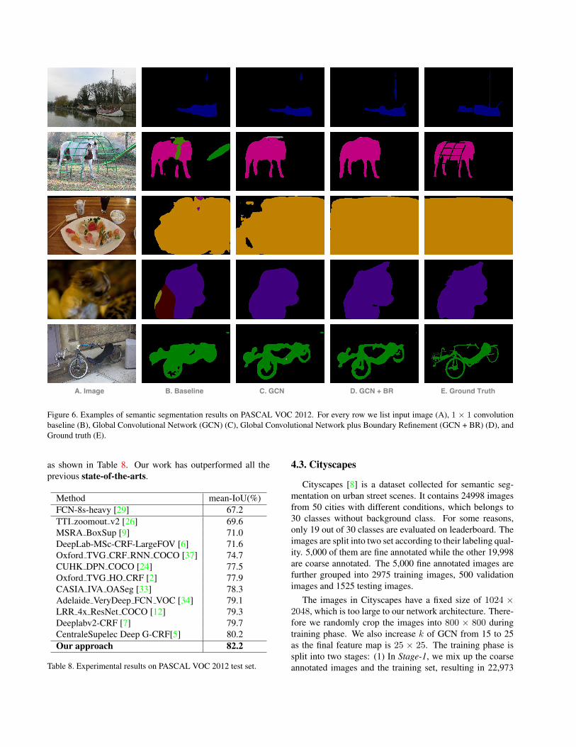
Our GCN + BR model clearly prevails, meanwhile thepost-processing multi-scale and denseCRF [18] also bringbenefits. Some visual comparisons are given in Figure 6.We also submit our best model to the on-line evaluationserver, obtaining 82.2% on PASCAL VOC 2012 test set,

Figure 6. Examples of semantic segmentation results on PASCAL VOC 2012. For every row we list input image (A), 1 × 1 convolutionbaseline (B), Global Convolutional Network (GCN) (C), Global Convolutional Network plus Boundary Refinement (GCN + BR) (D), andGround truth (E).

as shown in Table 8. Our work has outperformed all theprevious state-of-the-arts.

Method mean-IoU(%)FCN-8s-heavy [29] 67.2TTI zoomout v2 [26] 69.6MSRA BoxSup [9] 71.0DeepLab-MSc-CRF-LargeFOV [6] 71.6Oxford TVG CRF RNN COCO [37] 74.7CUHK DPN COCO [24] 77.5Oxford TVG HO CRF [2] 77.9CASIA IVA OASeg [33] 78.3Adelaide VeryDeep FCN VOC [34] 79.1LRR 4x ResNet COCO [12] 79.3Deeplabv2-CRF [7] 79.7CentraleSupelec Deep G-CRF[5] 80.2Our approach 82.2

Table 8. Experimental results on PASCAL VOC 2012 test set.

4.3. Cityscapes

Cityscapes [8] is a dataset collected for semantic seg-mentation on urban street scenes. It contains 24998 imagesfrom 50 cities with different conditions, which belongs to30 classes without background class. For some reasons,only 19 out of 30 classes are evaluated on leaderboard. Theimages are split into two set according to their labeling qual-ity. 5,000 of them are fine annotated while the other 19,998are coarse annotated. The 5,000 fine annotated images arefurther grouped into 2975 training images, 500 validationimages and 1525 testing images.

The images in Cityscapes have a fixed size of 1024 ×2048, which is too large to our network architecture. There-fore we randomly crop the images into 800 × 800 duringtraining phase. We also increase k of GCN from 15 to 25as the final feature map is 25 × 25. The training phase issplit into two stages: (1) In Stage-1, we mix up the coarseannotated images and the training set, resulting in 22,973

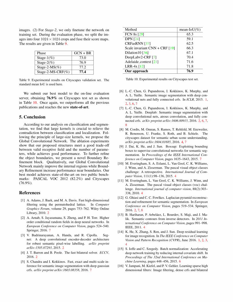
images. (2) For Stage-2, we only finetune the network ontraining set. During the evaluation phase, we split the im-ages into four 1024×1024 crops and fuse their score maps.The results are given in Table 9.

Phase GCN + BRStage-1(%) 73.0Stage-2(%) 76.9Stage-2-MS(%) 77.2Stage-2-MS-CRF(%) 77.4

Table 9. Experimental results on Cityscapes validation set. Thestandard mean IoU is used here.

We submit our best model to the on-line evaluationserver, obtaining 76.9% on Cityscapes test set as shownin Table 10. Once again, we outperforms all the previouspublications and reaches the new state-of-art.

5. ConclusionAccording to our analysis on classification and segmen-

tation, we find that large kernels is crucial to relieve thecontradiction between classification and localization. Fol-lowing the principle of large-size kernels, we propose theGlobal Convolutional Network. The ablation experimentsshow that our proposed structures meet a good trade-offbetween valid receptive field and the number of parame-ters, while achieves good performance. To further refinethe object boundaries, we present a novel Boundary Re-finement block. Qualitatively, our Global ConvolutionalNetwork mainly improve the internal regions while Bound-ary Refinement increase performance near boundaries. Ourbest model achieves state-of-the-art on two public bench-marks: PASCAL VOC 2012 (82.2%) and Cityscapes(76.9%).

References[1] A. Adams, J. Baek, and M. A. Davis. Fast high-dimensional

filtering using the permutohedral lattice. In ComputerGraphics Forum, volume 29, pages 753–762. Wiley OnlineLibrary, 2010. 2

[2] A. Arnab, S. Jayasumana, S. Zheng, and P. H. Torr. Higherorder conditional random fields in deep neural networks. InEuropean Conference on Computer Vision, pages 524–540.Springer, 2016. 7

[3] V. Badrinarayanan, A. Handa, and R. Cipolla. Seg-net: A deep convolutional encoder-decoder architecturefor robust semantic pixel-wise labelling. arXiv preprintarXiv:1505.07293, 2015. 2

[4] J. T. Barron and B. Poole. The fast bilateral solver. ECCV,2016. 2

[5] S. Chandra and I. Kokkinos. Fast, exact and multi-scale in-ference for semantic image segmentation with deep gaussiancrfs. arXiv preprint arXiv:1603.08358, 2016. 7

Method mean-IoU(%)FCN 8s [29] 65.3DPN [24] 59.1CRFasRNN [37] 62.5Scale invariant CNN + CRF [19] 66.3Dilation10 [36] 67.1DeepLabv2-CRF [7] 70.4Adelaide context [21] 71.6LRR-4x [12] 71.8Our approach 76.9

Table 10. Experimental results on Cityscapes test set.

[6] L.-C. Chen, G. Papandreou, I. Kokkinos, K. Murphy, andA. L. Yuille. Semantic image segmentation with deep con-volutional nets and fully connected crfs. In ICLR, 2015. 1,2, 3, 6, 7

[7] L.-C. Chen, G. Papandreou, I. Kokkinos, K. Murphy, andA. L. Yuille. Deeplab: Semantic image segmentation withdeep convolutional nets, atrous convolution, and fully con-nected crfs. arXiv preprint arXiv:1606.00915, 2016. 2, 6, 7,8

[8] M. Cordts, M. Omran, S. Ramos, T. Rehfeld, M. Enzweiler,R. Benenson, U. Franke, S. Roth, and B. Schiele. Thecityscapes dataset for semantic urban scene understanding.arXiv preprint arXiv:1604.01685, 2016. 4, 7

[9] J. Dai, K. He, and J. Sun. Boxsup: Exploiting boundingboxes to supervise convolutional networks for semantic seg-mentation. In Proceedings of the IEEE International Con-ference on Computer Vision, pages 1635–1643, 2015. 7

[10] M. Everingham, S. A. Eslami, L. Van Gool, C. K. Williams,J. Winn, and A. Zisserman. The pascal visual object classeschallenge: A retrospective. International Journal of Com-puter Vision, 111(1):98–136, 2015. 4

[11] M. Everingham, L. Van Gool, C. K. Williams, J. Winn, andA. Zisserman. The pascal visual object classes (voc) chal-lenge. International journal of computer vision, 88(2):303–338, 2010. 4

[12] G. Ghiasi and C. C. Fowlkes. Laplacian pyramid reconstruc-tion and refinement for semantic segmentation. In EuropeanConference on Computer Vision, pages 519–534. Springer,2016. 2, 7, 8

[13] B. Hariharan, P. Arbelaez, L. Bourdev, S. Maji, and J. Ma-lik. Semantic contours from inverse detectors. In 2011 In-ternational Conference on Computer Vision, pages 991–998.IEEE, 2011. 4

[14] K. He, X. Zhang, S. Ren, and J. Sun. Deep residual learningfor image recognition. In The IEEE Conference on ComputerVision and Pattern Recognition (CVPR), June 2016. 1, 2, 3,4

[15] S. Ioffe and C. Szegedy. Batch normalization: Acceleratingdeep network training by reducing internal covariate shift. InProceedings of The 32nd International Conference on Ma-chine Learning, pages 448–456, 2015. 6

[16] V. Jampani, M. Kiefel, and P. V. Gehler. Learning sparse highdimensional filters: Image filtering, dense crfs and bilateral

neural networks. In IEEE Conf. on Computer Vision andPattern Recognition (CVPR), June 2016. 2

[17] Y. Jia, E. Shelhamer, J. Donahue, S. Karayev, J. Long, R. Gir-shick, S. Guadarrama, and T. Darrell. Caffe: Convolu-tional architecture for fast feature embedding. arXiv preprintarXiv:1408.5093, 2014. 4

[18] V. Koltun. Efficient inference in fully connected crfs withgaussian edge potentials. Adv. Neural Inf. Process. Syst,2011. 2, 6

[19] I. Kreso, D. Causevic, J. Krapac, and S. Segvic. Con-volutional scale invariance for semantic segmentation. InGerman Conference on Pattern Recognition, pages 64–75.Springer, 2016. 8

[20] A. Krizhevsky, I. Sutskever, and G. E. Hinton. Imagenetclassification with deep convolutional neural networks. InAdvances in neural information processing systems, pages1097–1105, 2012. 2, 4

[21] G. Lin, C. Shen, A. van den Hengel, and I. Reid. Efficientpiecewise training of deep structured models for semanticsegmentation. In The IEEE Conference on Computer Visionand Pattern Recognition (CVPR), June 2016. 2, 8

[22] T.-Y. Lin, M. Maire, S. Belongie, J. Hays, P. Perona, D. Ra-manan, P. Dollar, and C. L. Zitnick. Microsoft coco: Com-mon objects in context. In European Conference on Com-puter Vision, pages 740–755. Springer, 2014. 6

[23] W. Liu, A. Rabinovich, and A. C. Berg. Parsenet: Lookingwider to see better. arXiv preprint arXiv:1506.04579, 2015.2

[24] Z. Liu, X. Li, P. Luo, C.-C. Loy, and X. Tang. Semantic im-age segmentation via deep parsing network. In Proceedingsof the IEEE International Conference on Computer Vision,pages 1377–1385, 2015. 2, 6, 7, 8

[25] J. Long, E. Shelhamer, and T. Darrell. Fully convolutionalnetworks for semantic segmentation. In Proceedings of theIEEE Conference on Computer Vision and Pattern Recogni-tion, pages 3431–3440, 2015. 1, 2, 3, 4

[26] M. Mostajabi, P. Yadollahpour, and G. Shakhnarovich. Feed-forward semantic segmentation with zoom-out features. InProceedings of the IEEE Conference on Computer Visionand Pattern Recognition, pages 3376–3385, 2015. 2, 7

[27] H. Noh, S. Hong, and B. Han. Learning deconvolution net-work for semantic segmentation. In Proceedings of the IEEEInternational Conference on Computer Vision, pages 1520–1528, 2015. 2, 3

[28] O. Russakovsky, J. Deng, H. Su, J. Krause, S. Satheesh,S. Ma, Z. Huang, A. Karpathy, A. Khosla, M. Bernstein,A. C. Berg, and L. Fei-Fei. ImageNet Large Scale VisualRecognition Challenge. International Journal of ComputerVision (IJCV), 115(3):211–252, 2015. 4, 6

[29] E. Shelhamer, J. Long, and T. Darrell. Fully convolutionalnetworks for semantic segmentation. 2016. 2, 7, 8

[30] K. Simonyan and A. Zisserman. Very deep convolutionalnetworks for large-scale image recognition. arXiv preprintarXiv:1409.1556, 2014. 1, 2, 5

[31] C. Szegedy, W. Liu, Y. Jia, P. Sermanet, S. Reed,D. Anguelov, D. Erhan, V. Vanhoucke, and A. Rabinovich.Going deeper with convolutions. In Proceedings of the IEEE

Conference on Computer Vision and Pattern Recognition,pages 1–9, 2015. 1, 2

[32] C. Szegedy, V. Vanhoucke, S. Ioffe, J. Shlens, and Z. Wojna.Rethinking the inception architecture for computer vision.arXiv preprint arXiv:1512.00567, 2015. 2, 3

[33] Y. Wang, J. Liu, Y. Li, J. Yan, and H. Lu. Objectness-awaresemantic segmentation. In Proceedings of the 2016 ACM onMultimedia Conference, pages 307–311. ACM, 2016. 7

[34] Z. Wu, C. Shen, and A. v. d. Hengel. High-performancesemantic segmentation using very deep fully convolutionalnetworks. arXiv preprint arXiv:1604.04339, 2016. 7

[35] S. Xie and Z. Tu. Holistically-nested edge detection. In Pro-ceedings of the IEEE International Conference on ComputerVision, pages 1395–1403, 2015. 3, 4

[36] F. Yu and V. Koltun. Multi-scale context aggregation by di-lated convolutions. arXiv preprint arXiv:1511.07122, 2015.2, 8

[37] S. Zheng, S. Jayasumana, B. Romera-Paredes, V. Vineet,Z. Su, D. Du, C. Huang, and P. H. Torr. Conditional randomfields as recurrent neural networks. In Proceedings of theIEEE International Conference on Computer Vision, pages1529–1537, 2015. 2, 6, 7, 8

[38] B. Zhou, A. Khosla, A. Lapedriza, A. Oliva, and A. Torralba.Object detectors emerge in deep scene cnns. arXiv preprintarXiv:1412.6856, 2014. 3, 4

Appendix.A ResNet50 and ResNet50-GCN

Component Output Size ResNet50 ResNet50-GCNconv1 112× 112 7× 7, 64, stride 2

res-2 56× 56

3× 3 max pool, stride 2 1× 1, 643× 3, 641× 1, 256

× 3

1× 1, 643× 3, 641× 1, 256

× 3

res-3 28× 28

1× 1, 1283× 3, 1281× 1, 512

× 4

1× 1, 1283× 3, 1281× 1, 512

× 4

res-4 14× 14

1× 1, 2563× 3, 2561× 1, 1024

× 6

(1× 5, 85) (5× 1, 85)(5× 1, 85) (1× 5, 85)

1× 1, 1024

× 6

res-5 7× 7

1× 1, 5123× 3, 5121× 1, 2048

× 3

(1× 7, 128) (7× 1, 128)(7× 1, 128) (1× 7, 128)

1× 1, 2048

× 3

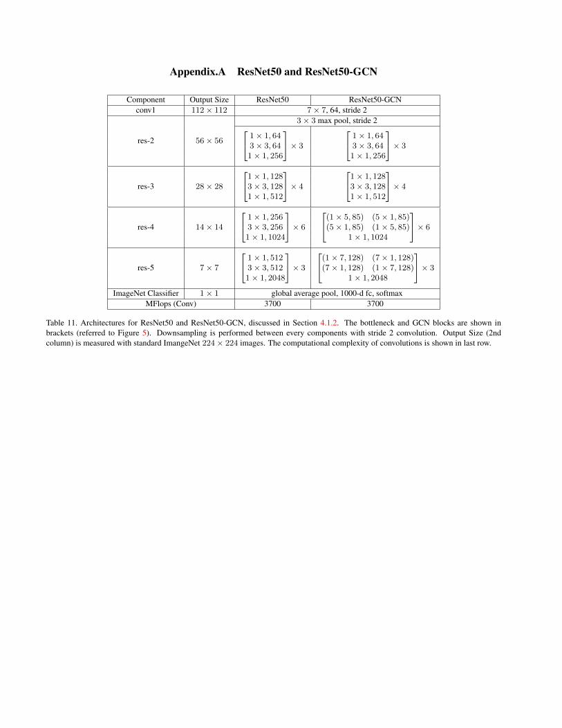
ImageNet Classifier 1× 1 global average pool, 1000-d fc, softmaxMFlops (Conv) 3700 3700

Table 11. Architectures for ResNet50 and ResNet50-GCN, discussed in Section 4.1.2. The bottleneck and GCN blocks are shown inbrackets (referred to Figure 5). Downsampling is performed between every components with stride 2 convolution. Output Size (2ndcolumn) is measured with standard ImangeNet 224× 224 images. The computational complexity of convolutions is shown in last row.

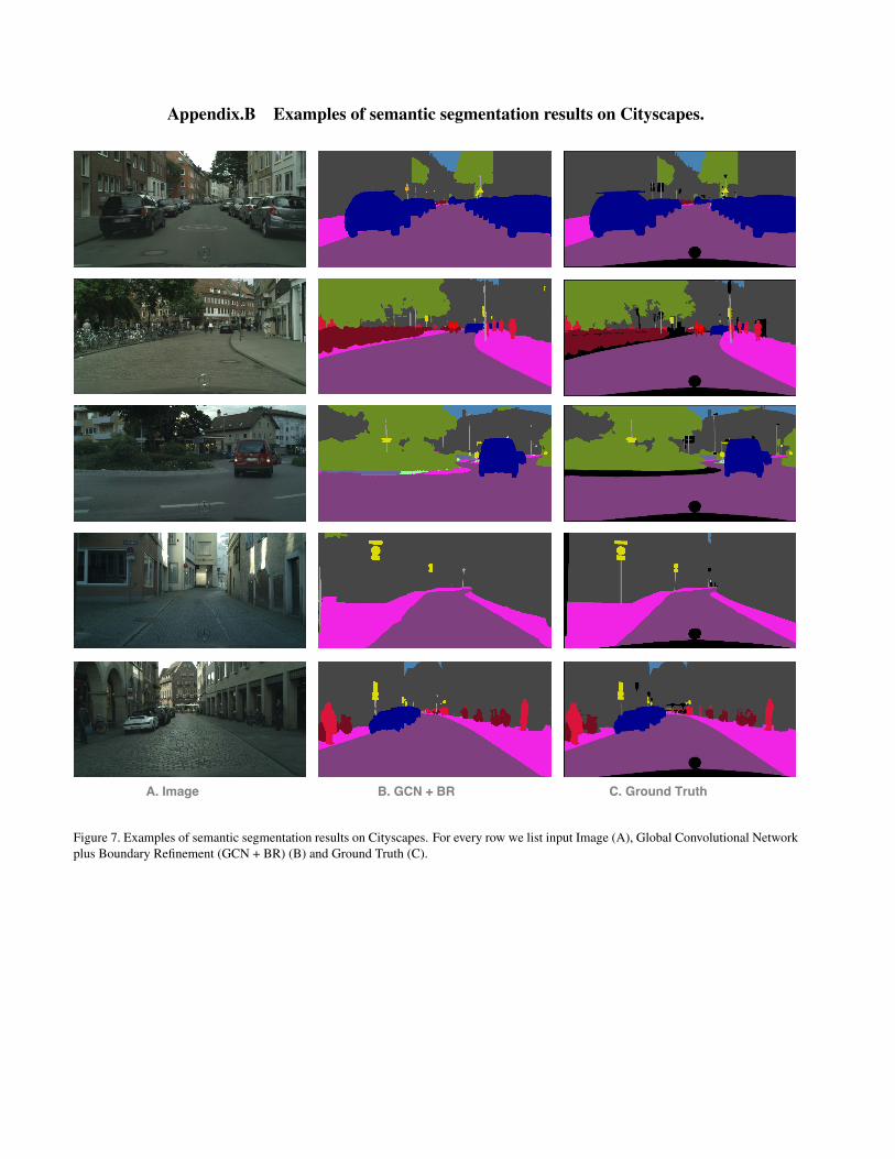
Appendix.B Examples of semantic segmentation results on Cityscapes.

Figure 7. Examples of semantic segmentation results on Cityscapes. For every row we list input Image (A), Global Convolutional Networkplus Boundary Refinement (GCN + BR) (B) and Ground Truth (C).