127
Parallel Computing Platforms Ananth Grama, Anshul Gupta, George Karypis, and Vipin Kumar To accompany the text ``Introduction to Parallel Computing'', Addison Wesley, 2003.
| Date post: | 20-Jul-2016 |
| Category: |
Documents |
| Upload: | florenceprasad |
| View: | 11 times |
| Download: | 5 times |
Parallel Computing Platforms
Ananth Grama, Anshul Gupta, George Karypis, and Vipin Kumar
To accompany the text ``Introduction to Parallel Computing'', Addison Wesley, 2003.
Topic Overview
• Implicit Parallelism: Trends in Microprocessor Architectures
• Limitations of Memory System Performance • Dichotomy of Parallel Computing Platforms • Communication Model of Parallel Platforms • Physical Organization of Parallel Platforms • Communication Costs in Parallel Machines • Messaging Cost Models and Routing Mechanisms • Mapping Techniques • Case Studies
Scope of Parallelism
• Conventional architectures coarsely comprise of a processor, memory system, and the datapath.
• Each of these components present significant performance bottlenecks.
• Parallelism addresses each of these components in significant ways.
• Different applications utilize different aspects of parallelism - e.g., data itensive applications utilize high aggregate throughput, server applications utilize high aggregate network bandwidth, and scientific applications typically utilize high processing and memory system performance.
• It is important to understand each of these performance bottlenecks.
Implicit Parallelism: Trends in Microprocessor Architectures
• Microprocessor clock speeds have posted impressive gains over the past two decades (two to three orders of magnitude).
• Higher levels of device integration have made available a large number of transistors.
• The question of how best to utilize these resources is an important one.
• Current processors use these resources in multiple functional units and execute multiple instructions in the same cycle.
• The precise manner in which these instructions are selected and executed provides impressive diversity in architectures.
Pipelining and Superscalar Execution
• Pipelining overlaps various stages of instruction execution to achieve performance.
• At a high level of abstraction, an instruction can be executed while the next one is being decoded and the next one is being fetched.
• This is akin to an assembly line for manufacture of cars.
Pipelining and Superscalar Execution
• Pipelining, however, has several limitations. • The speed of a pipeline is eventually limited by the
slowest stage. • For this reason, conventional processors rely on very
deep pipelines (20 stage pipelines in state-of-the-art Pentium processors).
• However, in typical program traces, every 5-6th instruction is a conditional jump! This requires very accurate branch prediction.
• The penalty of a misprediction grows with the depth of the pipeline, since a larger number of instructions will have to be flushed.
Pipelining and Superscalar Execution
• One simple way of alleviating these bottlenecks is to use multiple pipelines.
• The question then becomes one of selecting these instructions.
Superscalar Execution: An Example
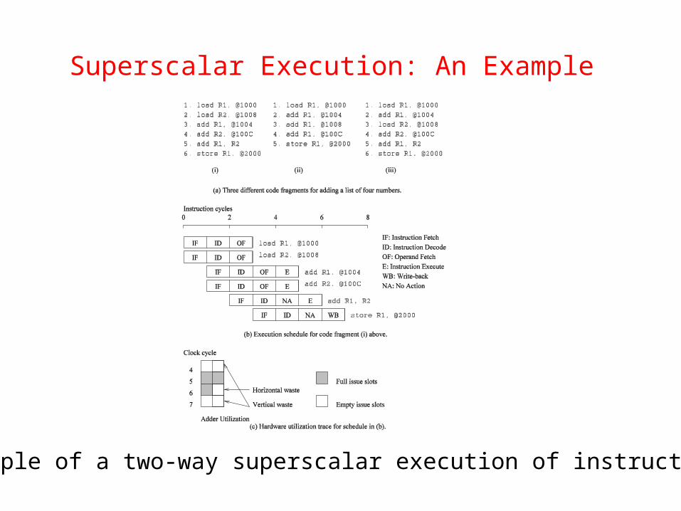
Example of a two-way superscalar execution of instructions.
Superscalar Execution: An Example
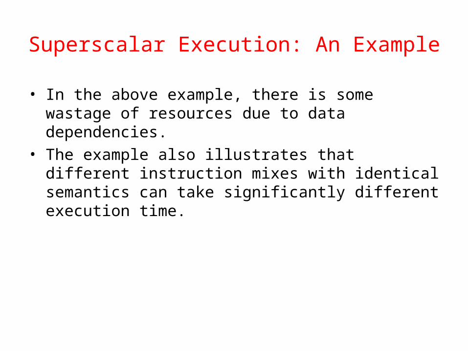
• In the above example, there is some wastage of resources due to data dependencies.
• The example also illustrates that different instruction mixes with identical semantics can take significantly different execution time.
Superscalar Execution
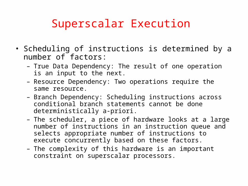
• Scheduling of instructions is determined by a number of factors: – True Data Dependency: The result of one operation is an input
to the next. – Resource Dependency: Two operations require the same
resource. – Branch Dependency: Scheduling instructions across conditional
branch statements cannot be done deterministically a-priori. – The scheduler, a piece of hardware looks at a large number of
instructions in an instruction queue and selects appropriate number of instructions to execute concurrently based on these factors.
– The complexity of this hardware is an important constraint on superscalar processors.
Superscalar Execution: Issue Mechanisms
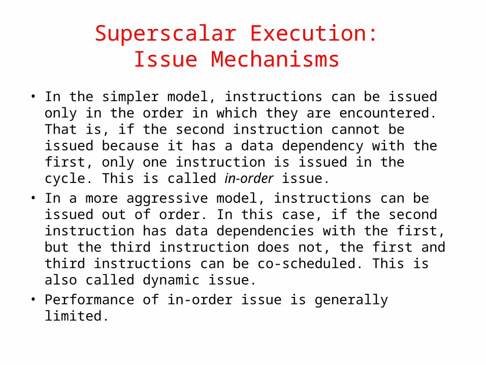
• In the simpler model, instructions can be issued only in the order in which they are encountered. That is, if the second instruction cannot be issued because it has a data dependency with the first, only one instruction is issued in the cycle. This is called in-order issue.
• In a more aggressive model, instructions can be issued out of order. In this case, if the second instruction has data dependencies with the first, but the third instruction does not, the first and third instructions can be co-scheduled. This is also called dynamic issue.
• Performance of in-order issue is generally limited.
Superscalar Execution: Efficiency Considerations
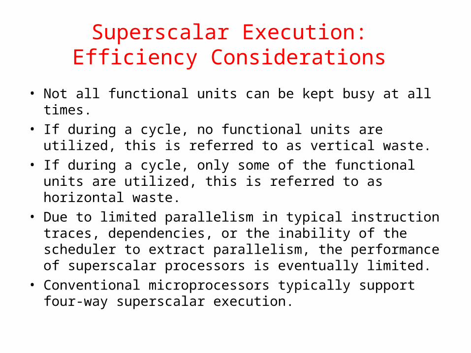
• Not all functional units can be kept busy at all times. • If during a cycle, no functional units are utilized, this is
referred to as vertical waste. • If during a cycle, only some of the functional units are
utilized, this is referred to as horizontal waste. • Due to limited parallelism in typical instruction traces,
dependencies, or the inability of the scheduler to extract parallelism, the performance of superscalar processors is eventually limited.
• Conventional microprocessors typically support four-way superscalar execution.
Very Long Instruction Word (VLIW) Processors
• The hardware cost and complexity of the superscalar scheduler is a major consideration in processor design.
• To address this issues, VLIW processors rely on compile time analysis to identify and bundle together instructions that can be executed concurrently.
• These instructions are packed and dispatched together, and thus the name very long instruction word.
• This concept was used with some commercial success in the Multiflow Trace machine (circa 1984).
• Variants of this concept are employed in the Intel IA64 processors.
Very Long Instruction Word (VLIW) Processors: Considerations
• Issue hardware is simpler. • Compiler has a bigger context from which to select co-
scheduled instructions. • Compilers, however, do not have runtime information
such as cache misses. Scheduling is, therefore, inherently conservative.
• Branch and memory prediction is more difficult. • VLIW performance is highly dependent on the compiler.
A number of techniques such as loop unrolling, speculative execution, branch prediction are critical.
• Typical VLIW processors are limited to 4-way to 8-way parallelism.
Limitations of Memory System Performance
• Memory system, and not processor speed, is often the bottleneck for many applications.
• Memory system performance is largely captured by two parameters, latency and bandwidth.
• Latency is the time from the issue of a memory request to the time the data is available at the processor.
• Bandwidth is the rate at which data can be pumped to the processor by the memory system.
Memory System Performance: Bandwidth and Latency
• It is very important to understand the difference between latency and bandwidth.
• Consider the example of a fire-hose. If the water comes out of the hose two seconds after the hydrant is turned on, the latency of the system is two seconds.
• Once the water starts flowing, if the hydrant delivers water at the rate of 5 gallons/second, the bandwidth of the system is 5 gallons/second.
• If you want immediate response from the hydrant, it is important to reduce latency.
• If you want to fight big fires, you want high bandwidth.
Memory Latency: An Example
• Consider a processor operating at 1 GHz (1 ns clock) connected to a DRAM with a latency of 100 ns (no caches). Assume that the processor has two multiply-add units and is capable of executing four instructions in each cycle of 1 ns. The following observations follow: – The peak processor rating is 4 GFLOPS. – Since the memory latency is equal to 100 cycles and block size
is one word, every time a memory request is made, the processor must wait 100 cycles before it can process the data.
Memory Latency: An Example
• On the above architecture, consider the problem of computing a dot-product of two vectors. – A dot-product computation performs one multiply-add on a single
pair of vector elements, i.e., each floating point operation requires one data fetch.
– It follows that the peak speed of this computation is limited to one floating point operation every 100 ns, or a speed of 10 MFLOPS, a very small fraction of the peak processor rating!
Improving Effective Memory Latency Using Caches
• Caches are small and fast memory elements between the processor and DRAM.
• This memory acts as a low-latency high-bandwidth storage.
• If a piece of data is repeatedly used, the effective latency of this memory system can be reduced by the cache.
• The fraction of data references satisfied by the cache is called the cache hit ratio of the computation on the system.
• Cache hit ratio achieved by a code on a memory system often determines its performance.
Impact of Caches: Example
Consider the architecture from the previous example. In this case, we introduce a cache of size 32 KB with a latency of 1 ns or one cycle. We use this setup to multiply two matrices A and B of dimensions 32 × 32. We have carefully chosen these numbers so that the cache is large enough to store matrices A and B, as well as the result matrix C.
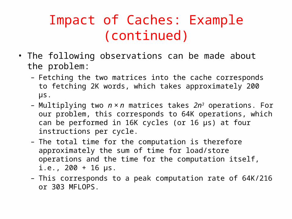
Impact of Caches: Example (continued)• The following observations can be made about the
problem:– Fetching the two matrices into the cache corresponds to fetching
2K words, which takes approximately 200 µs.– Multiplying two n × n matrices takes 2n3 operations. For our
problem, this corresponds to 64K operations, which can be performed in 16K cycles (or 16 µs) at four instructions per cycle.
– The total time for the computation is therefore approximately the sum of time for load/store operations and the time for the computation itself, i.e., 200 + 16 µs.
– This corresponds to a peak computation rate of 64K/216 or 303 MFLOPS.
Impact of Caches
• Repeated references to the same data item correspond to temporal locality.
• In our example, we had O(n2) data accesses and O(n3) computation. This asymptotic difference makes the above example particularly desirable for caches.
• Data reuse is critical for cache performance.
Impact of Memory Bandwidth
• Memory bandwidth is determined by the bandwidth of the memory bus as well as the memory units.
• Memory bandwidth can be improved by increasing the size of memory blocks.
• The underlying system takes l time units (where l is the latency of the system) to deliver b units of data (where b is the block size).
Impact of Memory Bandwidth: Example
• Consider the same setup as before, except in this case, the block size is 4 words instead of 1 word. We repeat the dot-product computation in this scenario:– Assuming that the vectors are laid out linearly in memory, eight
FLOPs (four multiply-adds) can be performed in 200 cycles.– This is because a single memory access fetches four
consecutive words in the vector.– Therefore, two accesses can fetch four elements of each of the
vectors. This corresponds to a FLOP every 25 ns, for a peak speed of 40 MFLOPS.
Impact of Memory Bandwidth
• It is important to note that increasing block size does not change latency of the system.
• Physically, the scenario illustrated here can be viewed as a wide data bus (4 words or 128 bits) connected to multiple memory banks.
• In practice, such wide buses are expensive to construct. • In a more practical system, consecutive words are sent
on the memory bus on subsequent bus cycles after the first word is retrieved.
Impact of Memory Bandwidth
• The above examples clearly illustrate how increased bandwidth results in higher peak computation rates.
• The data layouts were assumed to be such that consecutive data words in memory were used by successive instructions (spatial locality of reference).
• If we take a data-layout centric view, computations must be reordered to enhance spatial locality of reference.
Impact of Memory Bandwidth: Example
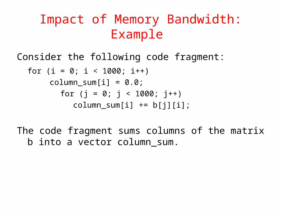
Consider the following code fragment: for (i = 0; i < 1000; i++)
column_sum[i] = 0.0; for (j = 0; j < 1000; j++) column_sum[i] += b[j][i];
The code fragment sums columns of the matrix b into a vector column_sum.
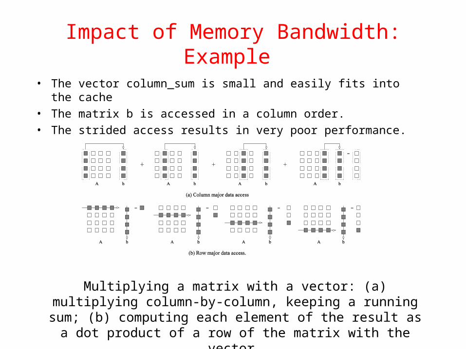
Impact of Memory Bandwidth: Example • The vector column_sum is small and easily fits into the cache • The matrix b is accessed in a column order. • The strided access results in very poor performance.
Multiplying a matrix with a vector: (a) multiplying column-by-column, keeping a running sum; (b) computing each element of the result as a dot product of a row of the matrix with the vector.
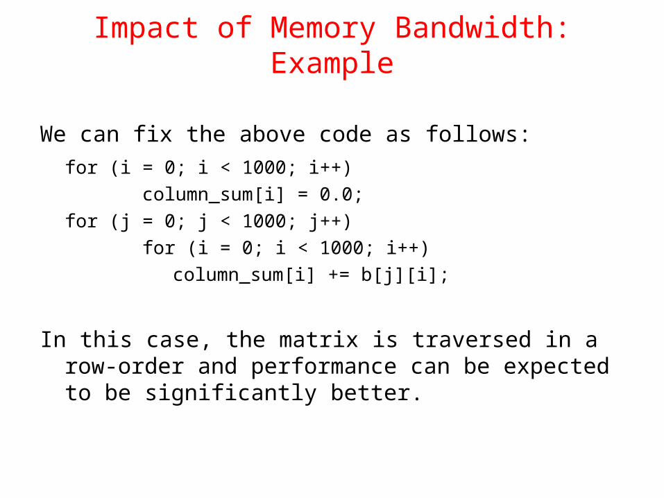
Impact of Memory Bandwidth: Example
We can fix the above code as follows: for (i = 0; i < 1000; i++)
column_sum[i] = 0.0;for (j = 0; j < 1000; j++)
for (i = 0; i < 1000; i++) column_sum[i] += b[j][i];
In this case, the matrix is traversed in a row-order and performance can be expected to be significantly better.
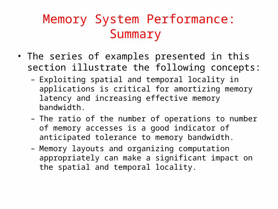
Memory System Performance: Summary
• The series of examples presented in this section illustrate the following concepts: – Exploiting spatial and temporal locality in applications is critical
for amortizing memory latency and increasing effective memory bandwidth.
– The ratio of the number of operations to number of memory accesses is a good indicator of anticipated tolerance to memory bandwidth.
– Memory layouts and organizing computation appropriately can make a significant impact on the spatial and temporal locality.
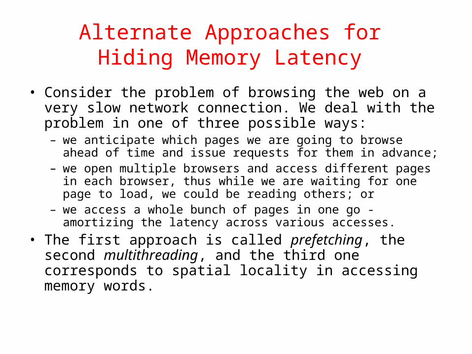
Alternate Approaches for Hiding Memory Latency
• Consider the problem of browsing the web on a very slow network connection. We deal with the problem in one of three possible ways: – we anticipate which pages we are going to browse ahead of time
and issue requests for them in advance; – we open multiple browsers and access different pages in each
browser, thus while we are waiting for one page to load, we could be reading others; or
– we access a whole bunch of pages in one go - amortizing the latency across various accesses.
• The first approach is called prefetching, the second multithreading, and the third one corresponds to spatial locality in accessing memory words.
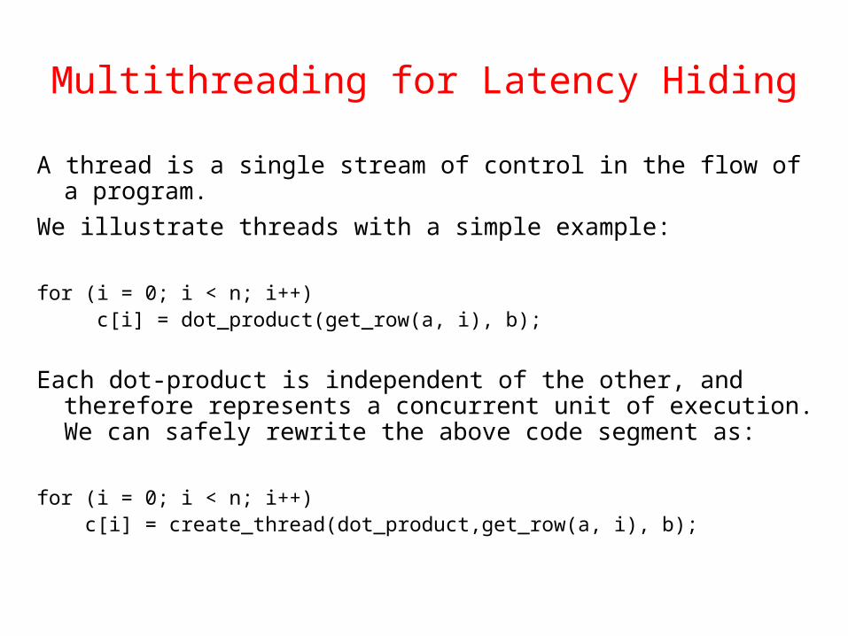
Multithreading for Latency Hiding
A thread is a single stream of control in the flow of a program. We illustrate threads with a simple example:
for (i = 0; i < n; i++) c[i] = dot_product(get_row(a, i), b);
Each dot-product is independent of the other, and therefore represents a concurrent unit of execution. We can safely rewrite the above code segment as:
for (i = 0; i < n; i++) c[i] = create_thread(dot_product,get_row(a, i), b);
Multithreading for Latency Hiding: Example
• In the code, the first instance of this function accesses a pair of vector elements and waits for them.
• In the meantime, the second instance of this function can access two other vector elements in the next cycle, and so on.
• After l units of time, where l is the latency of the memory system, the first function instance gets the requested data from memory and can perform the required computation.
• In the next cycle, the data items for the next function instance arrive, and so on. In this way, in every clock cycle, we can perform a computation.
Multithreading for Latency Hiding
• The execution schedule in the previous example is predicated upon two assumptions: the memory system is capable of servicing multiple outstanding requests, and the processor is capable of switching threads at every cycle.
• It also requires the program to have an explicit specification of concurrency in the form of threads.
• Machines such as the HEP and Tera rely on multithreaded processors that can switch the context of execution in every cycle. Consequently, they are able to hide latency effectively.
Prefetching for Latency Hiding
• Misses on loads cause programs to stall. • Why not advance the loads so that by the time the data
is actually needed, it is already there! • The only drawback is that you might need more space to
store advanced loads. • However, if the advanced loads are overwritten, we are
no worse than before!
Tradeoffs of Multithreading and Prefetching
• Multithreading and prefetching are critically impacted by the memory bandwidth. Consider the following example: – Consider a computation running on a machine with a 1 GHz
clock, 4-word cache line, single cycle access to the cache, and 100 ns latency to DRAM. The computation has a cache hit ratio at 1 KB of 25% and at 32 KB of 90%. Consider two cases: first, a single threaded execution in which the entire cache is available to the serial context, and second, a multithreaded execution with 32 threads where each thread has a cache residency of 1 KB.
– If the computation makes one data request in every cycle of 1 ns, you may notice that the first scenario requires 400MB/s of memory bandwidth and the second, 3GB/s.
Tradeoffs of Multithreading and Prefetching
• Bandwidth requirements of a multithreaded system may increase very significantly because of the smaller cache residency of each thread.
• Multithreaded systems become bandwidth bound instead of latency bound.
• Multithreading and prefetching only address the latency problem and may often exacerbate the bandwidth problem.
• Multithreading and prefetching also require significantly more hardware resources in the form of storage.
Explicitly Parallel Platforms
Dichotomy of Parallel Computing Platforms
• An explicitly parallel program must specify concurrency and interaction between concurrent subtasks.
• The former is sometimes also referred to as the control structure and the latter as the communication model.
Control Structure of Parallel Programs
• Parallelism can be expressed at various levels of granularity - from instruction level to processes.
• Between these extremes exist a range of models, along with corresponding architectural support.
Control Structure of Parallel Programs
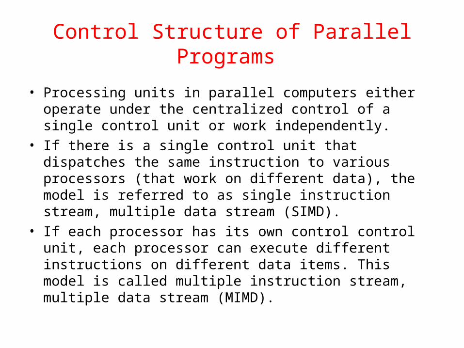
• Processing units in parallel computers either operate under the centralized control of a single control unit or work independently.
• If there is a single control unit that dispatches the same instruction to various processors (that work on different data), the model is referred to as single instruction stream, multiple data stream (SIMD).
• If each processor has its own control control unit, each processor can execute different instructions on different data items. This model is called multiple instruction stream, multiple data stream (MIMD).
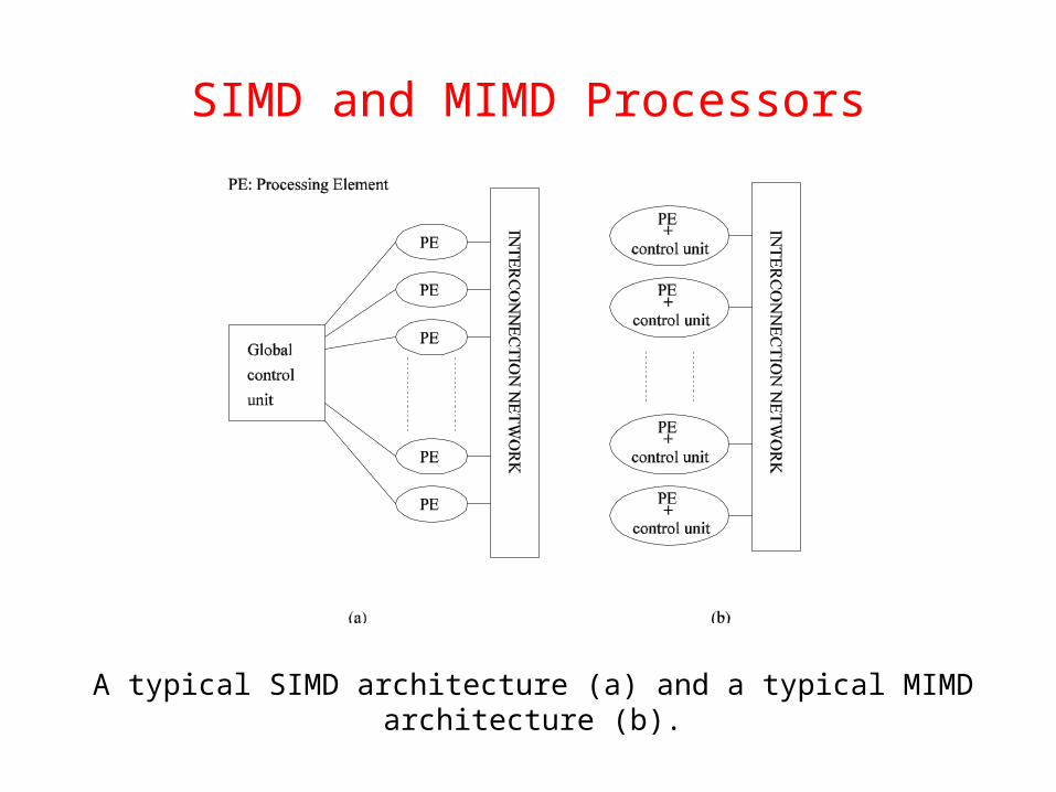
SIMD and MIMD Processors
A typical SIMD architecture (a) and a typical MIMD architecture (b).
SIMD Processors • Some of the earliest parallel computers such as the Illiac IV,
MPP, DAP, CM-2, and MasPar MP-1 belonged to this class of machines.
• Variants of this concept have found use in co-processing units such as the MMX units in Intel processors and DSP chips such as the Sharc.
• SIMD relies on the regular structure of computations (such as those in image processing).
• It is often necessary to selectively turn off operations on certain data items. For this reason, most SIMD programming paradigms allow for an ``activity mask'', which determines if a processor should participate in a computation or not.
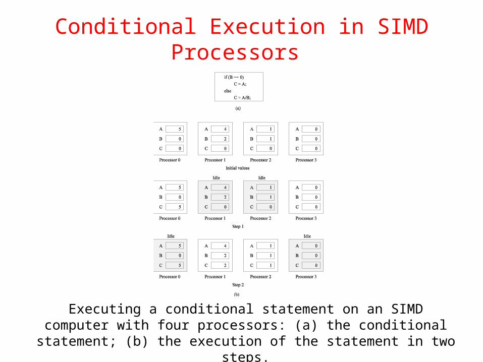
Conditional Execution in SIMD Processors
Executing a conditional statement on an SIMD computer with four processors: (a) the conditional statement; (b) the execution of the
statement in two steps.
MIMD Processors
• In contrast to SIMD processors, MIMD processors can execute different programs on different processors.
• A variant of this, called single program multiple data streams (SPMD) executes the same program on different processors.
• It is easy to see that SPMD and MIMD are closely related in terms of programming flexibility and underlying architectural support.
• Examples of such platforms include current generation Sun Ultra Servers, SGI Origin Servers, multiprocessor PCs, workstation clusters, and the IBM SP.
SIMD-MIMD Comparison
• SIMD computers require less hardware than MIMD computers (single control unit).
• However, since SIMD processors ae specially designed, they tend to be expensive and have long design cycles.
• Not all applications are naturally suited to SIMD processors.
• In contrast, platforms supporting the SPMD paradigm can be built from inexpensive off-the-shelf components with relatively little effort in a short amount of time.
Communication Model of Parallel Platforms
• There are two primary forms of data exchange between parallel tasks - accessing a shared data space and exchanging messages.
• Platforms that provide a shared data space are called shared-address-space machines or multiprocessors.
• Platforms that support messaging are also called message passing platforms or multicomputers.
Shared-Address-Space Platforms
• Part (or all) of the memory is accessible to all processors.
• Processors interact by modifying data objects stored in this shared-address-space.
• If the time taken by a processor to access any memory word in the system global or local is identical, the platform is classified as a uniform memory access (UMA), else, a non-uniform memory access (NUMA) machine.
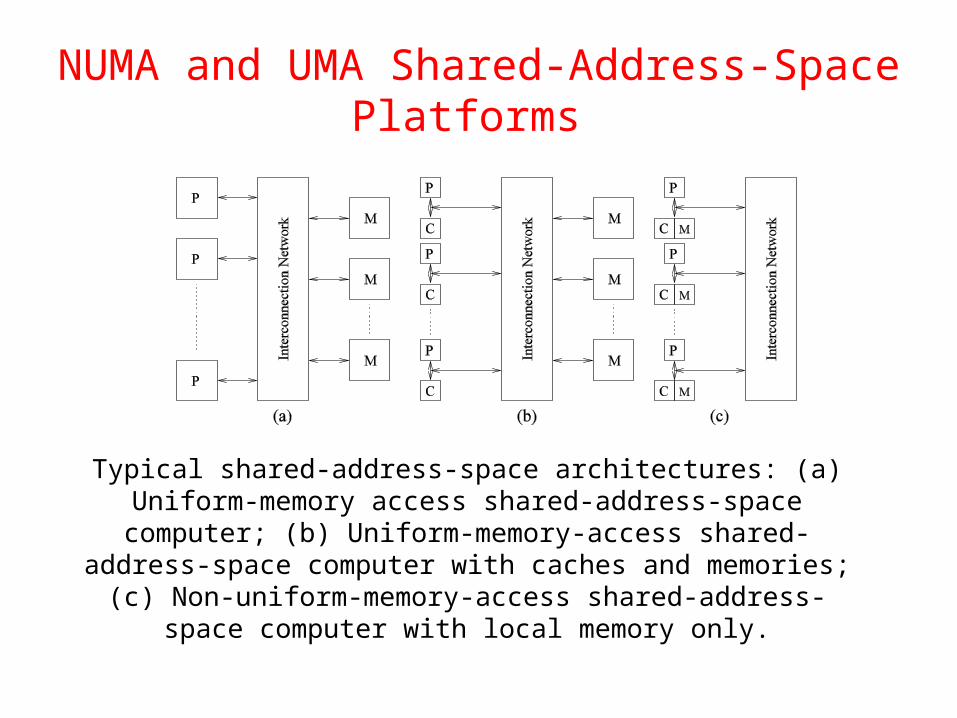
NUMA and UMA Shared-Address-Space Platforms
Typical shared-address-space architectures: (a) Uniform-memory access shared-address-space computer; (b) Uniform-memory-
access shared-address-space computer with caches and memories; (c) Non-uniform-memory-access shared-address-
space computer with local memory only.
NUMA and UMA Shared-Address-Space Platforms
• The distinction between NUMA and UMA platforms is important from the point of view of algorithm design. NUMA machines require locality from underlying algorithms for performance.
• Programming these platforms is easier since reads and writes are implicitly visible to other processors.
• However, read-write data to shared data must be coordinated (this will be discussed in greater detail when we talk about threads programming).
• Caches in such machines require coordinated access to multiple copies. This leads to the cache coherence problem.
• A weaker model of these machines provides an address map, but not coordinated access. These models are called non cache coherent shared address space machines.
Shared-Address-Space vs.
Shared Memory Machines • It is important to note the difference between the terms
shared address space and shared memory. • We refer to the former as a programming abstraction and
to the latter as a physical machine attribute. • It is possible to provide a shared address space using a
physically distributed memory.
Message-Passing Platforms
• These platforms comprise of a set of processors and their own (exclusive) memory.
• Instances of such a view come naturally from clustered workstations and non-shared-address-space multicomputers.
• These platforms are programmed using (variants of) send and receive primitives.
• Libraries such as MPI and PVM provide such primitives.
Message Passing vs.
Shared Address Space Platforms • Message passing requires little hardware support, other
than a network. • Shared address space platforms can easily emulate
message passing. The reverse is more difficult to do (in an efficient manner).
Physical Organization of Parallel Platforms
We begin this discussion with an ideal parallel machine called Parallel Random Access Machine, or PRAM.
Architecture of an Ideal Parallel Computer
• A natural extension of the Random Access Machine (RAM) serial architecture is the Parallel Random Access Machine, or PRAM.
• PRAMs consist of p processors and a global memory of unbounded size that is uniformly accessible to all processors.
• Processors share a common clock but may execute different instructions in each cycle.
Architecture of an Ideal Parallel Computer
• Depending on how simultaneous memory accesses are handled, PRAMs can be divided into four subclasses. – Exclusive-read, exclusive-write (EREW) PRAM. – Concurrent-read, exclusive-write (CREW) PRAM. – Exclusive-read, concurrent-write (ERCW) PRAM. – Concurrent-read, concurrent-write (CRCW) PRAM.
Architecture of an Ideal Parallel Computer
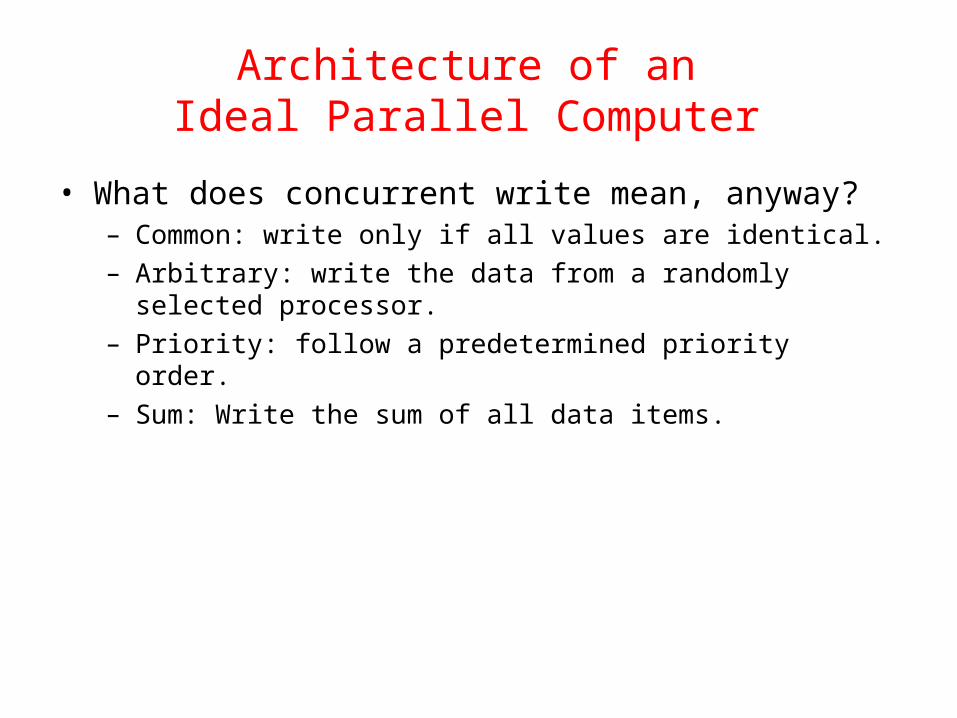
• What does concurrent write mean, anyway? – Common: write only if all values are identical. – Arbitrary: write the data from a randomly selected processor. – Priority: follow a predetermined priority order. – Sum: Write the sum of all data items.
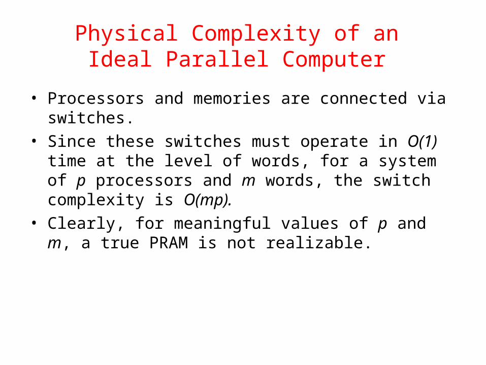
Physical Complexity of an Ideal Parallel Computer
• Processors and memories are connected via switches.• Since these switches must operate in O(1) time at the
level of words, for a system of p processors and m words, the switch complexity is O(mp).
• Clearly, for meaningful values of p and m, a true PRAM is not realizable.
Interconnection Networks for Parallel Computers
• Interconnection networks carry data between processors and to memory.
• Interconnects are made of switches and links (wires, fiber).
• Interconnects are classified as static or dynamic. • Static networks consist of point-to-point communication
links among processing nodes and are also referred to as direct networks.
• Dynamic networks are built using switches and communication links. Dynamic networks are also referred to as indirect networks.
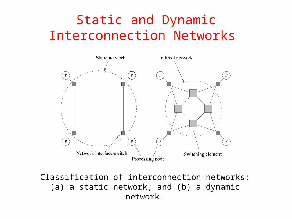
Static and DynamicInterconnection Networks
Classification of interconnection networks: (a) a static network; and (b) a dynamic network.
Interconnection Networks
• Switches map a fixed number of inputs to outputs. • The total number of ports on a switch is the degree of
the switch. • The cost of a switch grows as the square of the degree
of the switch, the peripheral hardware linearly as the degree, and the packaging costs linearly as the number of pins.
Interconnection Networks: Network Interfaces
• Processors talk to the network via a network interface. • The network interface may hang off the I/O bus or the
memory bus. • In a physical sense, this distinguishes a cluster from a
tightly coupled multicomputer. • The relative speeds of the I/O and memory buses impact
the performance of the network.
Network Topologies
• A variety of network topologies have been proposed and implemented.
• These topologies tradeoff performance for cost. • Commercial machines often implement hybrids of
multiple topologies for reasons of packaging, cost, and available components.
Network Topologies: Buses
• Some of the simplest and earliest parallel machines used buses.
• All processors access a common bus for exchanging data.
• The distance between any two nodes is O(1) in a bus. The bus also provides a convenient broadcast media.
• However, the bandwidth of the shared bus is a major bottleneck.
• Typical bus based machines are limited to dozens of nodes. Sun Enterprise servers and Intel Pentium based shared-bus multiprocessors are examples of such architectures.
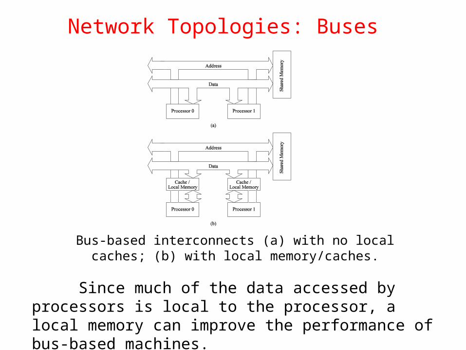
Network Topologies: Buses
Bus-based interconnects (a) with no local caches; (b) with local memory/caches.
Since much of the data accessed by processors is local to the processor, a local memory can improve the performance of bus-based machines.
Network Topologies: Crossbars
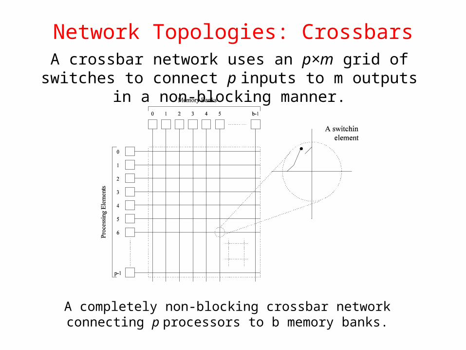
A completely non-blocking crossbar network connecting p processors to b memory banks.
A crossbar network uses an p×m grid of switches to connect p inputs to m outputs in a non-blocking manner.
Network Topologies: Crossbars
• The cost of a crossbar of p processors grows as O(p2).• This is generally difficult to scale for large values of p.• Examples of machines that employ crossbars include the
Sun Ultra HPC 10000 and the Fujitsu VPP500.
Network Topologies: Multistage Networks
• Crossbars have excellent performance scalability but poor cost scalability.
• Buses have excellent cost scalability, but poor performance scalability.
• Multistage interconnects strike a compromise between these extremes.
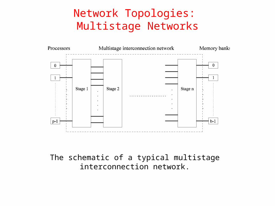
Network Topologies: Multistage Networks
The schematic of a typical multistage interconnection network.
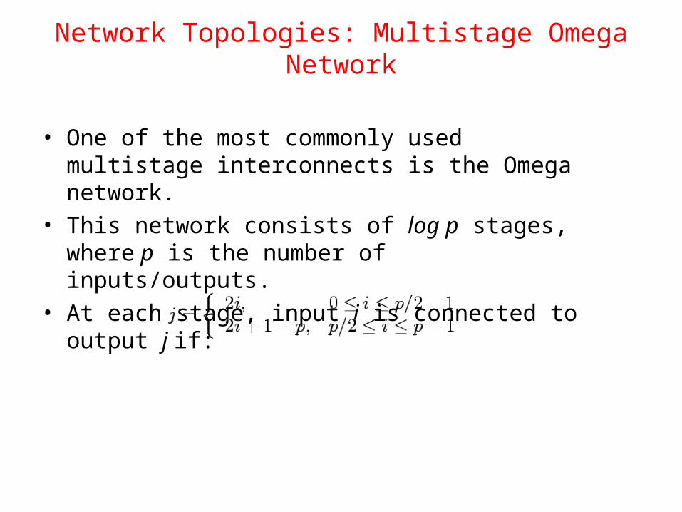
Network Topologies: Multistage Omega Network
• One of the most commonly used multistage interconnects is the Omega network.
• This network consists of log p stages, where p is the number of inputs/outputs.
• At each stage, input i is connected to output j if:
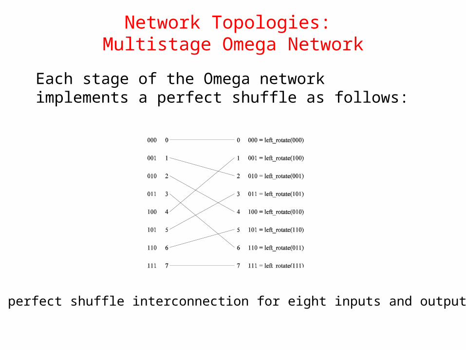
Network Topologies: Multistage Omega Network
Each stage of the Omega network implements a perfect shuffle as follows:
A perfect shuffle interconnection for eight inputs and outputs.
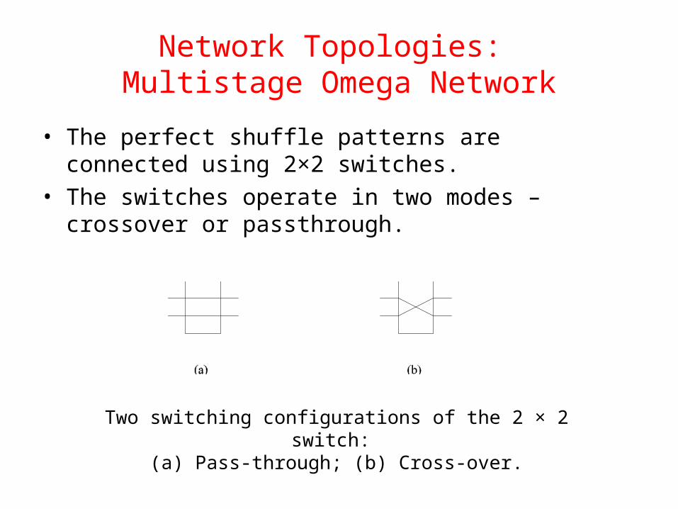
Network Topologies: Multistage Omega Network
• The perfect shuffle patterns are connected using 2×2 switches.
• The switches operate in two modes – crossover or passthrough.
Two switching configurations of the 2 × 2 switch: (a) Pass-through; (b) Cross-over.
Network Topologies: Multistage Omega Network
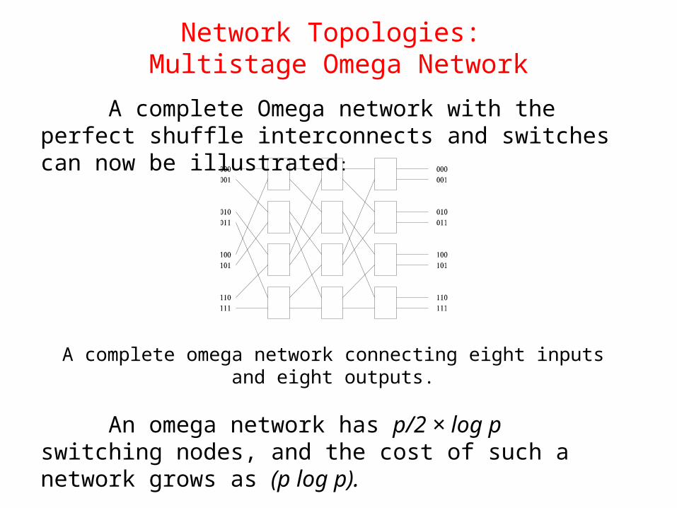
A complete omega network connecting eight inputs and eight outputs.
An omega network has p/2 × log p switching nodes, and the cost of such a network grows as (p log p).
A complete Omega network with the perfect shuffle interconnects and switches can now be illustrated:
Network Topologies: Multistage Omega Network – Routing
• Let s be the binary representation of the source and d be that of the destination processor.
• The data traverses the link to the first switching node. If the most significant bits of s and d are the same, then the data is routed in pass-through mode by the switch else, it switches to crossover.
• This process is repeated for each of the log p switching stages.
• Note that this is not a non-blocking switch.
Network Topologies: Multistage Omega Network – Routing
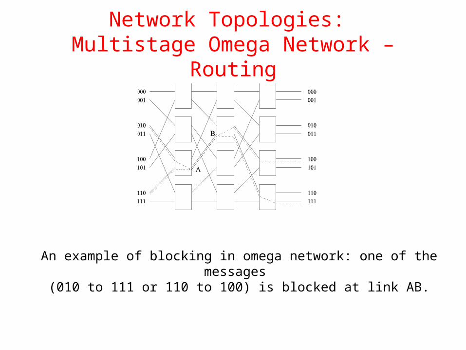
An example of blocking in omega network: one of the messages (010 to 111 or 110 to 100) is blocked at link AB.
Network Topologies: Completely Connected Network
• Each processor is connected to every other processor.• The number of links in the network scales as O(p2).• While the performance scales very well, the hardware
complexity is not realizable for large values of p.• In this sense, these networks are static counterparts of
crossbars.
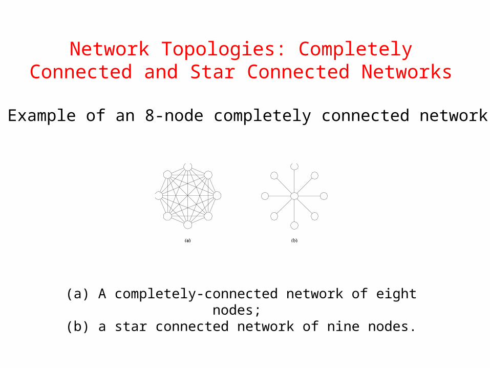
Network Topologies: Completely Connected and Star Connected Networks
Example of an 8-node completely connected network.
(a) A completely-connected network of eight nodes; (b) a star connected network of nine nodes.
Network Topologies: Star Connected Network
• Every node is connected only to a common node at the center.
• Distance between any pair of nodes is O(1). However, the central node becomes a bottleneck.
• In this sense, star connected networks are static counterparts of buses.
Network Topologies: Linear Arrays, Meshes, and k-d Meshes
• In a linear array, each node has two neighbors, one to its left and one to its right. If the nodes at either end are connected, we refer to it as a 1-D torus or a ring.
• A generalization to 2 dimensions has nodes with 4 neighbors, to the north, south, east, and west.
• A further generalization to d dimensions has nodes with 2d neighbors.
• A special case of a d-dimensional mesh is a hypercube. Here, d = log p, where p is the total number of nodes.
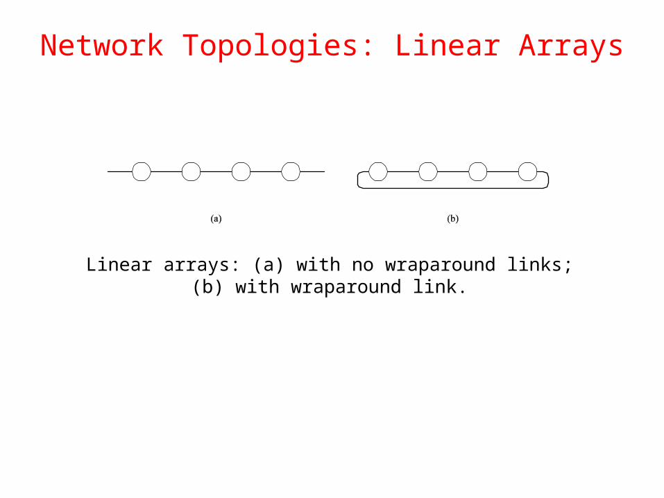
Network Topologies: Linear Arrays
Linear arrays: (a) with no wraparound links; (b) with wraparound link.
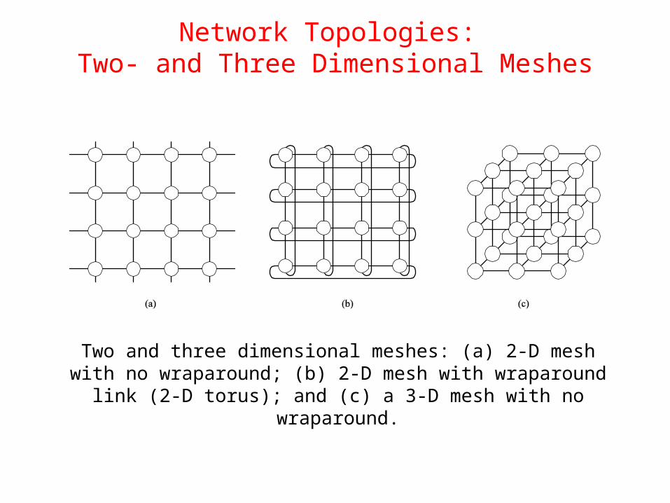
Network Topologies: Two- and Three Dimensional Meshes
Two and three dimensional meshes: (a) 2-D mesh with no wraparound; (b) 2-D mesh with wraparound link (2-D torus); and
(c) a 3-D mesh with no wraparound.
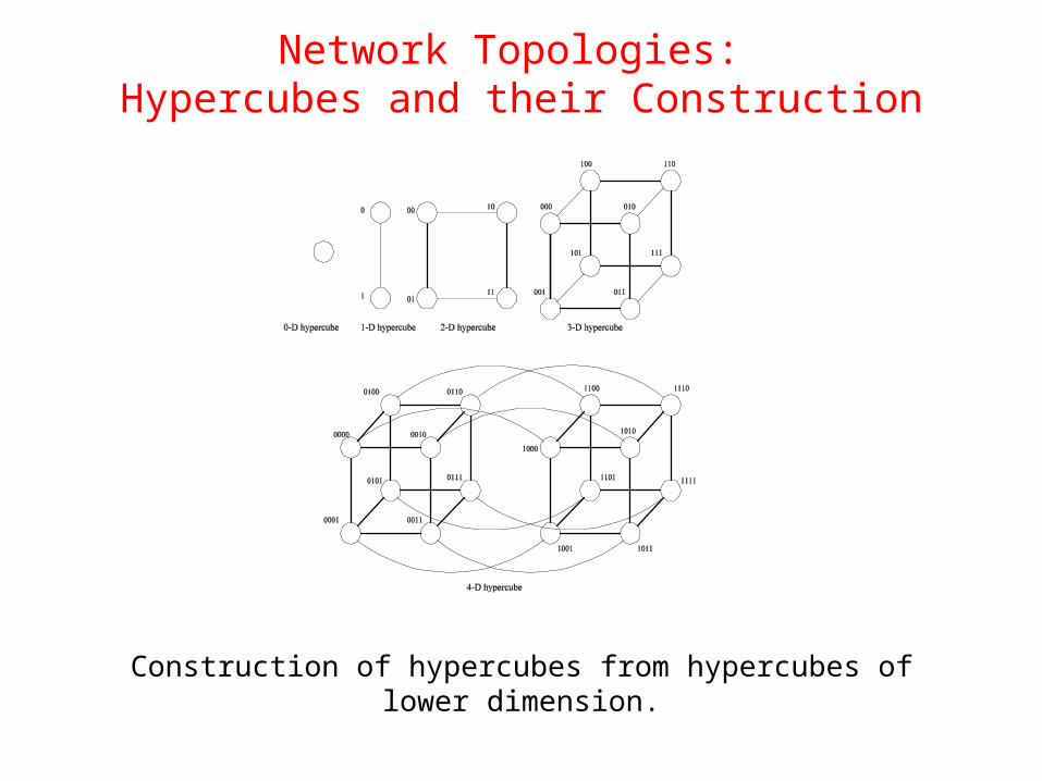
Network Topologies: Hypercubes and their Construction
Construction of hypercubes from hypercubes of lower dimension.
Network Topologies: Properties of Hypercubes
• The distance between any two nodes is at most log p.• Each node has log p neighbors.• The distance between two nodes is given by the number
of bit positions at which the two nodes differ.
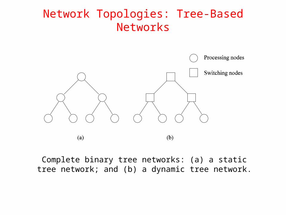
Network Topologies: Tree-Based Networks
Complete binary tree networks: (a) a static tree network; and (b) a dynamic tree network.
Network Topologies: Tree Properties
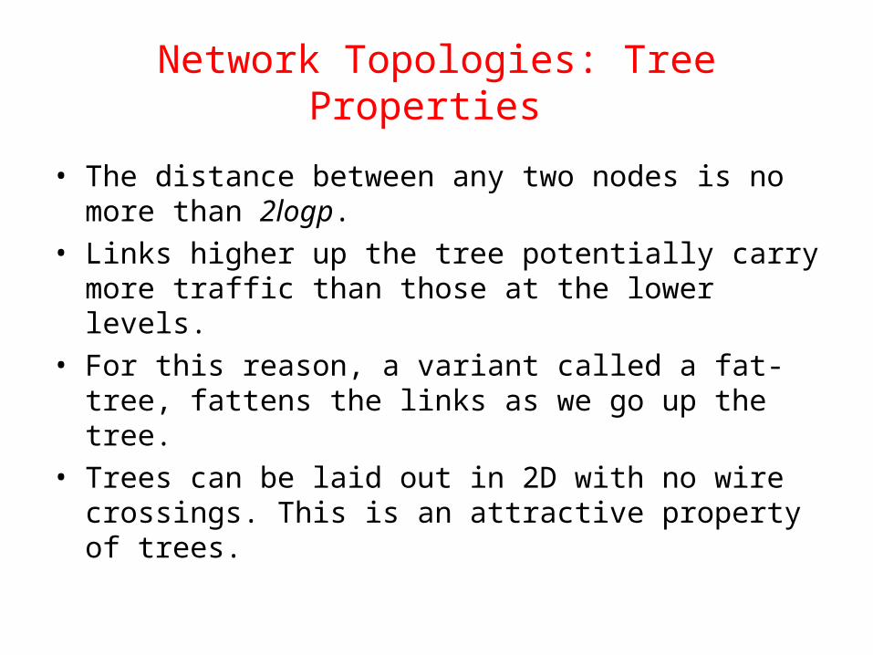
• The distance between any two nodes is no more than 2logp.
• Links higher up the tree potentially carry more traffic than those at the lower levels.
• For this reason, a variant called a fat-tree, fattens the links as we go up the tree.
• Trees can be laid out in 2D with no wire crossings. This is an attractive property of trees.
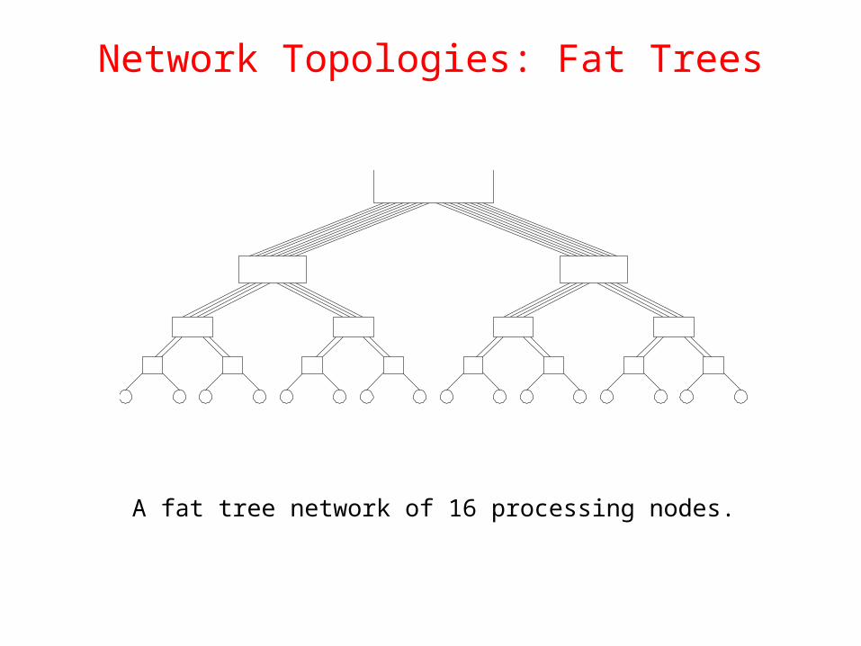
Network Topologies: Fat Trees
A fat tree network of 16 processing nodes.
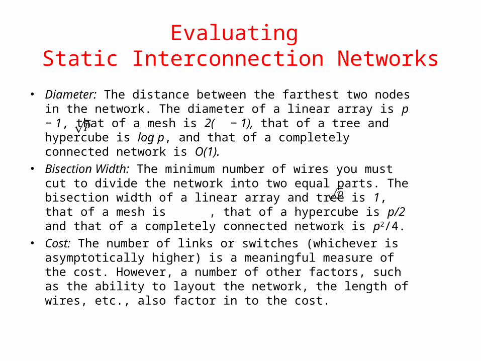
Evaluating Static Interconnection Networks
• Diameter: The distance between the farthest two nodes in the network. The diameter of a linear array is p − 1, that of a mesh is 2( − 1), that of a tree and hypercube is log p, and that of a completely connected network is O(1).
• Bisection Width: The minimum number of wires you must cut to divide the network into two equal parts. The bisection width of a linear array and tree is 1, that of a mesh is , that of a hypercube is p/2 and that of a completely connected network is p2/4.
• Cost: The number of links or switches (whichever is asymptotically higher) is a meaningful measure of the cost. However, a number of other factors, such as the ability to layout the network, the length of wires, etc., also factor in to the cost.
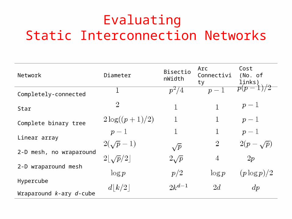
Evaluating Static Interconnection Networks
Network Diameter BisectionWidth
Arc Connectivity
Cost (No. of links)
Completely-connected
Star
Complete binary tree
Linear array
2-D mesh, no wraparound
2-D wraparound mesh
Hypercube
Wraparound k-ary d-cube
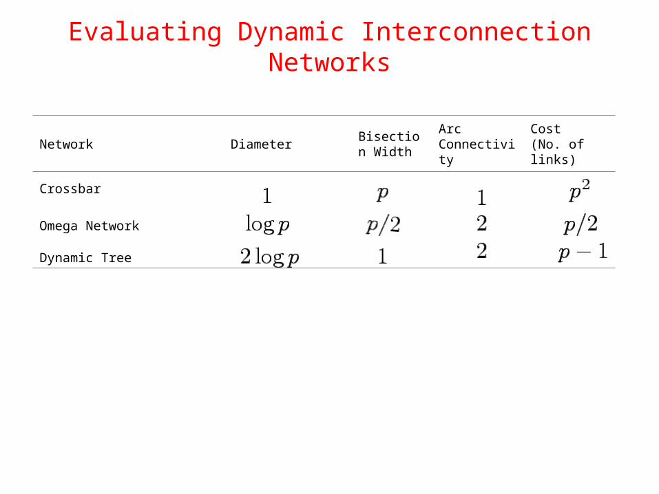
Evaluating Dynamic Interconnection Networks
Network Diameter Bisection Width
Arc Connectivity
Cost (No. of links)
Crossbar
Omega Network
Dynamic Tree
Cache Coherence in Multiprocessor Systems
• Interconnects provide basic mechanisms for data transfer.
• In the case of shared address space machines, additional hardware is required to coordinate access to data that might have multiple copies in the network.
• The underlying technique must provide some guarantees on the semantics.
• This guarantee is generally one of serializability, i.e., there exists some serial order of instruction execution that corresponds to the parallel schedule.
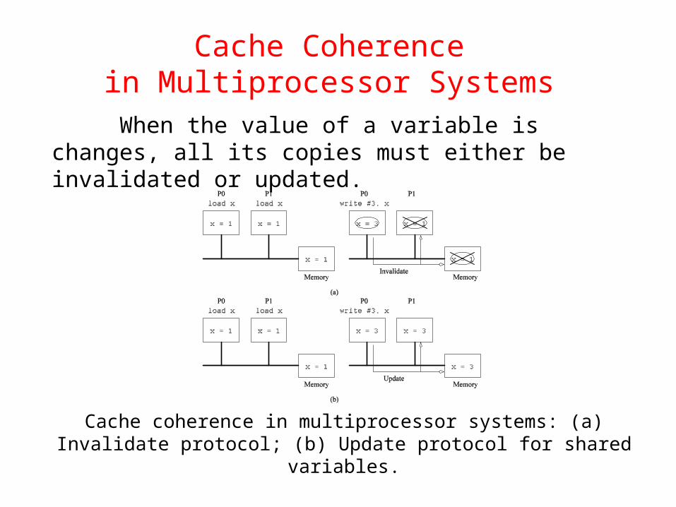
Cache Coherence in Multiprocessor Systems
Cache coherence in multiprocessor systems: (a) Invalidate protocol; (b) Update protocol for shared variables.
When the value of a variable is changes, all its copies must either be invalidated or updated.
Cache Coherence: Update and Invalidate Protocols
• If a processor just reads a value once and does not need it again, an update protocol may generate significant overhead.
• If two processors make interleaved test and updates to a variable, an update protocol is better.
• Both protocols suffer from false sharing overheads (two words that are not shared, however, they lie on the same cache line).
• Most current machines use invalidate protocols.
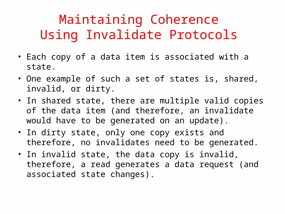
Maintaining Coherence Using Invalidate Protocols
• Each copy of a data item is associated with a state. • One example of such a set of states is, shared, invalid,
or dirty. • In shared state, there are multiple valid copies of the
data item (and therefore, an invalidate would have to be generated on an update).
• In dirty state, only one copy exists and therefore, no invalidates need to be generated.
• In invalid state, the data copy is invalid, therefore, a read generates a data request (and associated state changes).
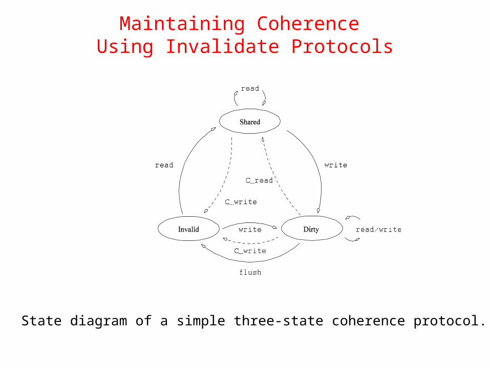
Maintaining Coherence Using Invalidate Protocols
State diagram of a simple three-state coherence protocol.
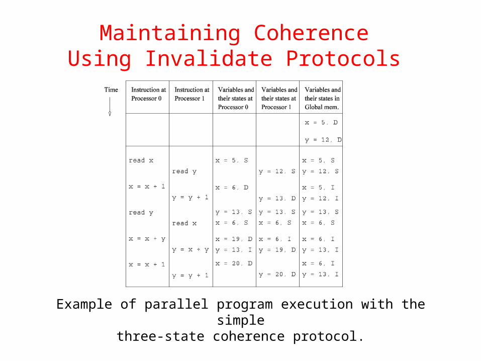
Maintaining Coherence Using Invalidate Protocols
Example of parallel program execution with the simplethree-state coherence protocol.
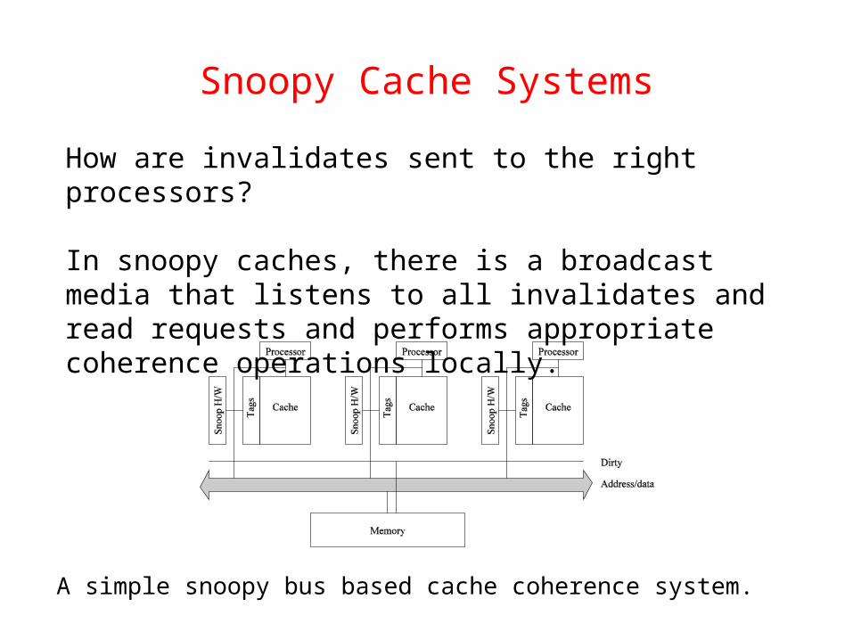
Snoopy Cache SystemsHow are invalidates sent to the right processors?
In snoopy caches, there is a broadcast media that listens to all invalidates and read requests and performs appropriate coherence operations locally.
A simple snoopy bus based cache coherence system.
Performance of Snoopy Caches
• Once copies of data are tagged dirty, all subsequent operations can be performed locally on the cache without generating external traffic.
• If a data item is read by a number of processors, it transitions to the shared state in the cache and all subsequent read operations become local.
• If processors read and update data at the same time, they generate coherence requests on the bus - which is ultimately bandwidth limited.
Directory Based Systems
• In snoopy caches, each coherence operation is sent to all processors. This is an inherent limitation.
• Why not send coherence requests to only those processors that need to be notified?
• This is done using a directory, which maintains a presence vector for each data item (cache line) along with its global state.
Directory Based Systems
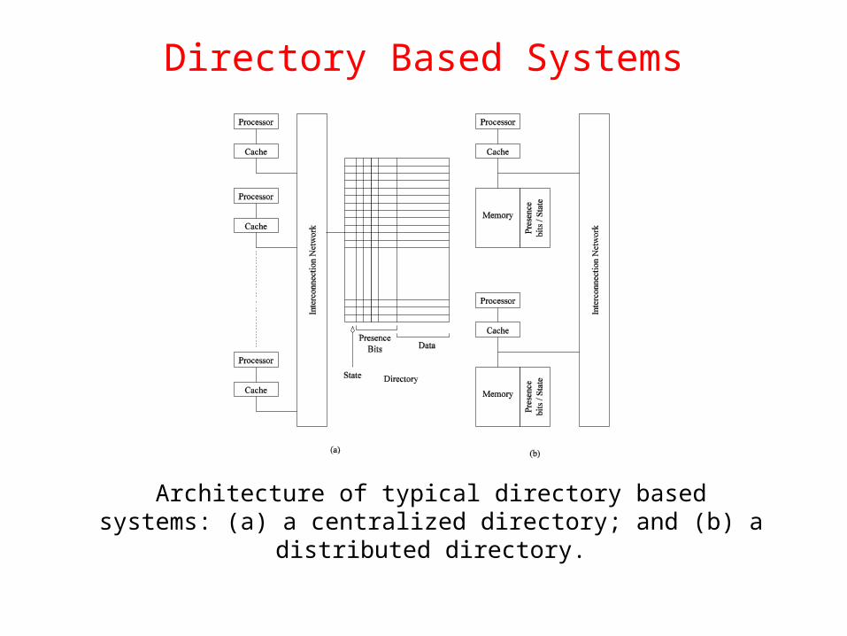
Architecture of typical directory based systems: (a) a centralized directory; and (b) a distributed directory.

Performance of Directory Based Schemes
• The need for a broadcast media is replaced by the directory.
• The additional bits to store the directory may add significant overhead.
• The underlying network must be able to carry all the coherence requests.
• The directory is a point of contention, therefore, distributed directory schemes must be used.
Communication Costs in Parallel Machines
• Along with idling and contention, communication is a major overhead in parallel programs.
• The cost of communication is dependent on a variety of features including the programming model semantics, the network topology, data handling and routing, and associated software protocols.
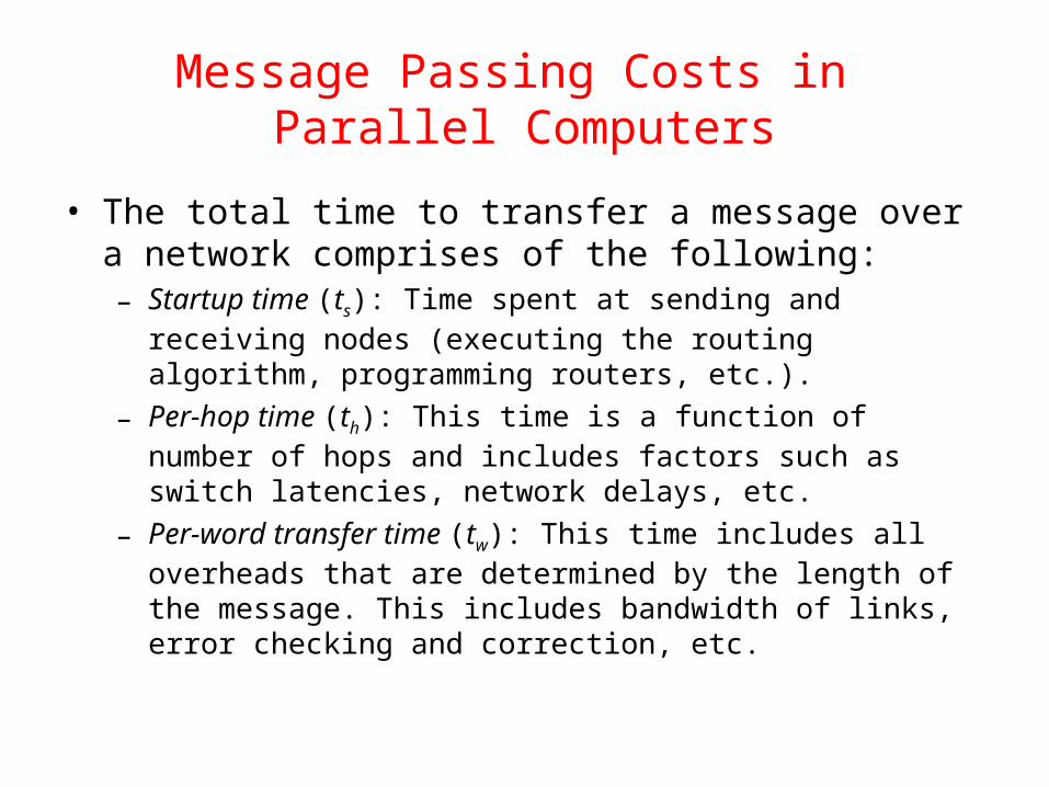
Message Passing Costs in Parallel Computers
• The total time to transfer a message over a network comprises of the following:– Startup time (ts): Time spent at sending and receiving nodes
(executing the routing algorithm, programming routers, etc.).– Per-hop time (th): This time is a function of number of hops and
includes factors such as switch latencies, network delays, etc.– Per-word transfer time (tw): This time includes all overheads that
are determined by the length of the message. This includes bandwidth of links, error checking and correction, etc.
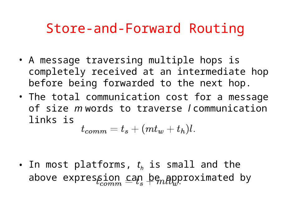
Store-and-Forward Routing
• A message traversing multiple hops is completely received at an intermediate hop before being forwarded to the next hop.
• The total communication cost for a message of size m words to traverse l communication links is
• In most platforms, th is small and the above expression can be approximated by
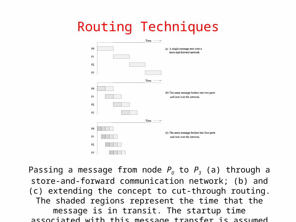
Routing Techniques
Passing a message from node P0 to P3 (a) through a store-and-forward communication network; (b) and (c) extending the concept to cut-through routing. The shaded regions represent the time that
the message is in transit. The startup time associated with this message transfer is assumed to be zero.
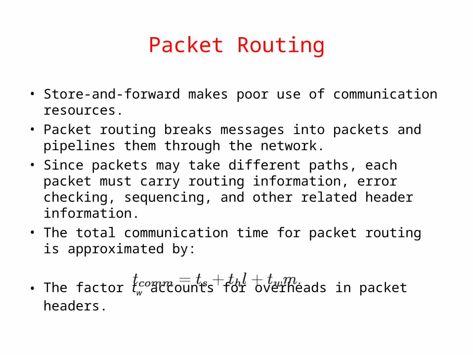
Packet Routing
• Store-and-forward makes poor use of communication resources.
• Packet routing breaks messages into packets and pipelines them through the network.
• Since packets may take different paths, each packet must carry routing information, error checking, sequencing, and other related header information.
• The total communication time for packet routing is approximated by:
• The factor tw accounts for overheads in packet headers.
Cut-Through Routing
• Takes the concept of packet routing to an extreme by further dividing messages into basic units called flits.
• Since flits are typically small, the header information must be minimized.
• This is done by forcing all flits to take the same path, in sequence.
• A tracer message first programs all intermediate routers. All flits then take the same route.
• Error checks are performed on the entire message, as opposed to flits.
• No sequence numbers are needed.
Cut-Through Routing
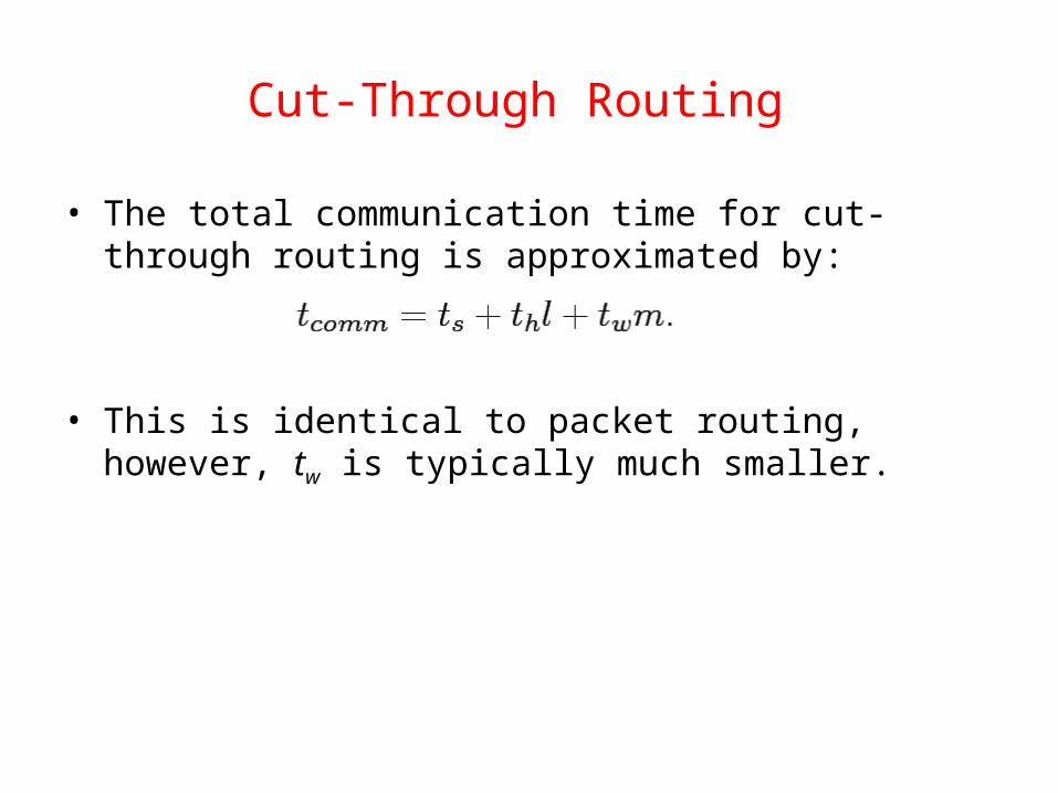
• The total communication time for cut-through routing is approximated by:
• This is identical to packet routing, however, tw is typically much smaller.
Simplified Cost Model for Communicating Messages
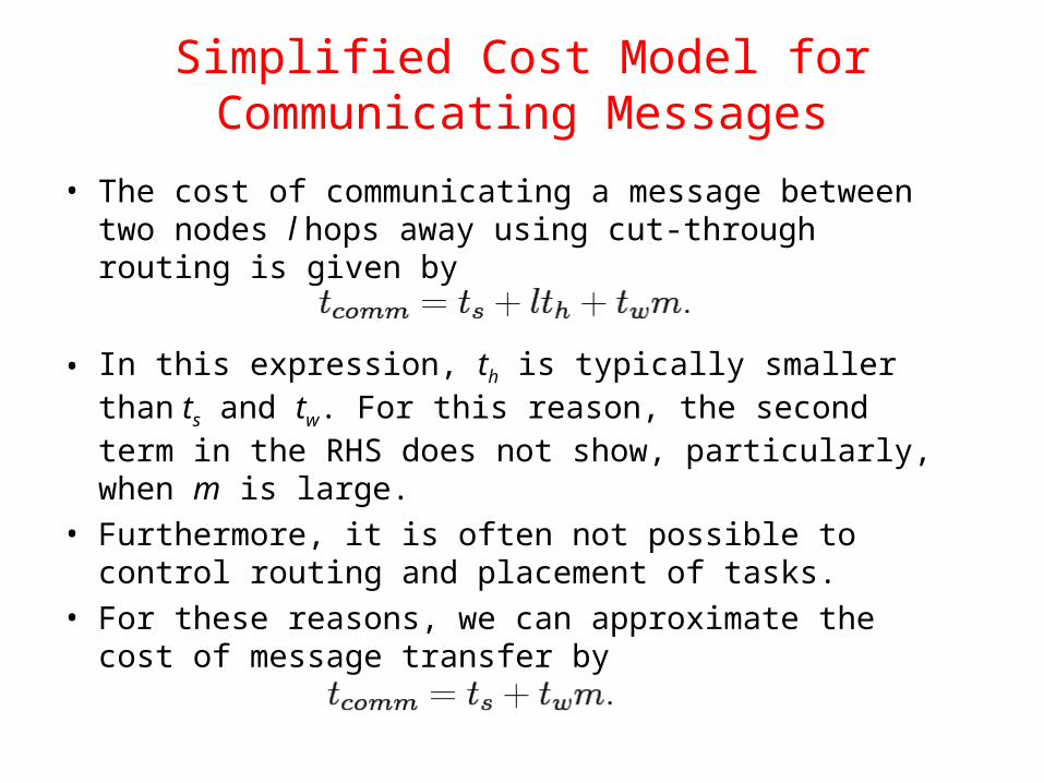
• The cost of communicating a message between two nodes l hops away using cut-through routing is given by
• In this expression, th is typically smaller than ts and tw. For this reason, the second term in the RHS does not show, particularly, when m is large.
• Furthermore, it is often not possible to control routing and placement of tasks.
• For these reasons, we can approximate the cost of message transfer by
Simplified Cost Model for Communicating Messages
• It is important to note that the original expression for communication time is valid for only uncongested networks.
• If a link takes multiple messages, the corresponding tw term must be scaled up by the number of messages.
• Different communication patterns congest different networks to varying extents.
• It is important to understand and account for this in the communication time accordingly.
Cost Models for Shared Address Space Machines
• While the basic messaging cost applies to these machines as well, a number of other factors make accurate cost modeling more difficult.
• Memory layout is typically determined by the system. • Finite cache sizes can result in cache thrashing. • Overheads associated with invalidate and update
operations are difficult to quantify. • Spatial locality is difficult to model. • Prefetching can play a role in reducing the overhead
associated with data access. • False sharing and contention are difficult to model.
Routing Mechanisms for Interconnection Networks
• How does one compute the route that a message takes from source to destination? – Routing must prevent deadlocks - for this reason, we use
dimension-ordered or e-cube routing. – Routing must avoid hot-spots - for this reason, two-step routing
is often used. In this case, a message from source s to destination d is first sent to a randomly chosen intermediate processor i and then forwarded to destination d.
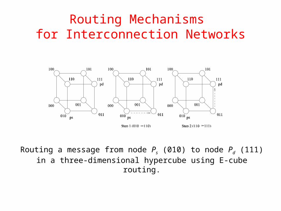
Routing Mechanisms for Interconnection Networks
Routing a message from node Ps (010) to node Pd (111) in a three-dimensional hypercube using E-cube routing.
Mapping Techniques for Graphs
• Often, we need to embed a known communication pattern into a given interconnection topology.
• We may have an algorithm designed for one network, which we are porting to another topology.
For these reasons, it is useful to understand mapping between graphs.
Mapping Techniques for Graphs: Metrics
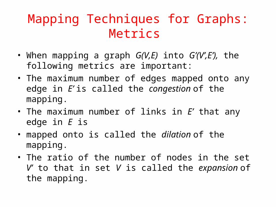
• When mapping a graph G(V,E) into G’(V’,E’), the following metrics are important:
• The maximum number of edges mapped onto any edge in E’ is called the congestion of the mapping.
• The maximum number of links in E’ that any edge in E is• mapped onto is called the dilation of the mapping.• The ratio of the number of nodes in the set V’ to that in
set V is called the expansion of the mapping.
Embedding a Linear Array into a Hypercube
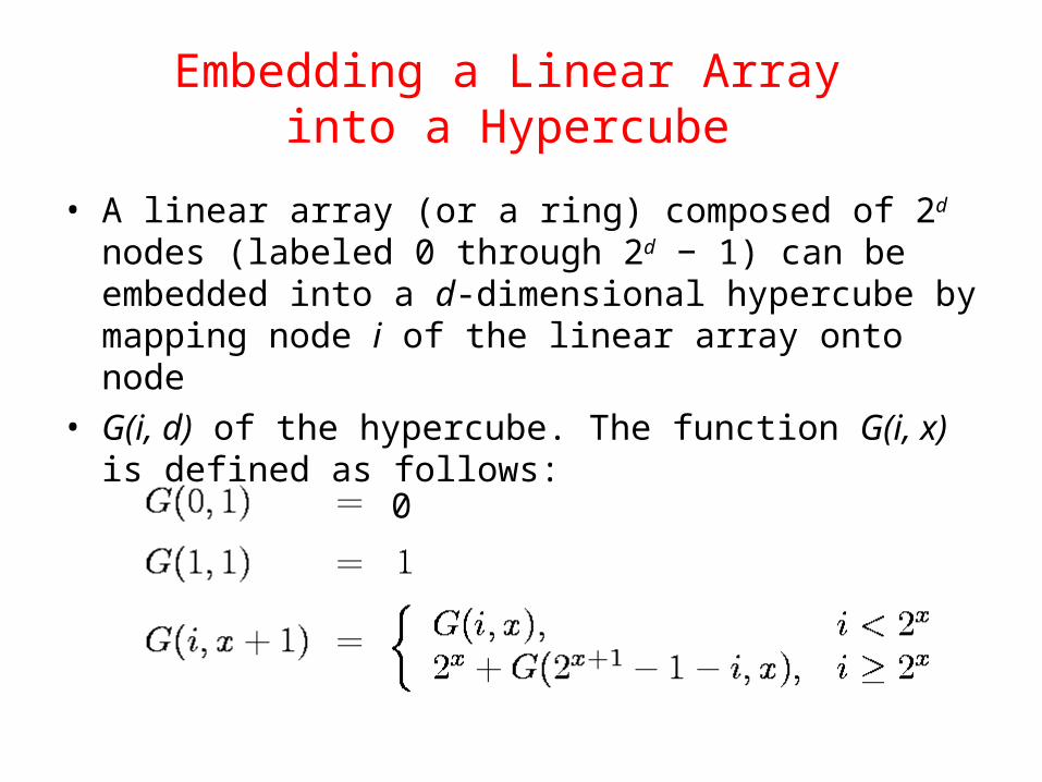
• A linear array (or a ring) composed of 2d nodes (labeled 0 through 2d − 1) can be embedded into a d-dimensional hypercube by mapping node i of the linear array onto node
• G(i, d) of the hypercube. The function G(i, x) is defined as follows:
0
Embedding a Linear Array into a Hypercube
The function G is called the binary reflected Gray code (RGC).
Since adjoining entries (G(i, d) and G(i + 1, d)) differ from each other at only one bit position, corresponding processors are mapped to neighbors in a hypercube. Therefore, the congestion, dilation, and expansion of the mapping are all 1.
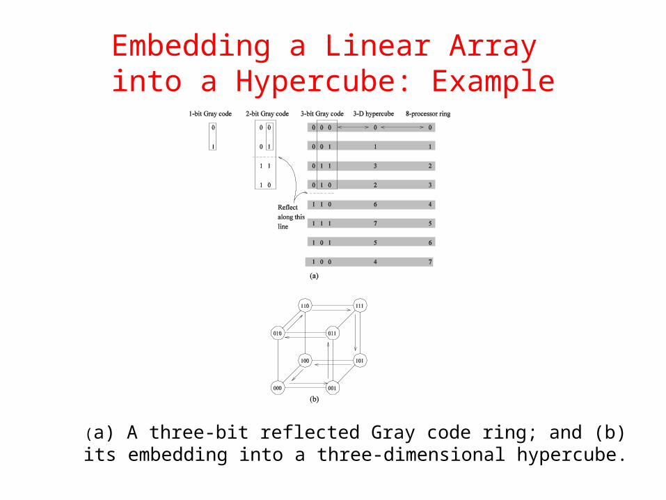
Embedding a Linear Array into a Hypercube: Example
(a) A three-bit reflected Gray code ring; and (b) its embedding into a three-dimensional hypercube.
Embedding a Mesh into a Hypercube
• A 2r × 2s wraparound mesh can be mapped to a 2r+s-node hypercube by mapping node (i, j) of the mesh onto node G(i, r− 1) || G(j, s − 1) of the hypercube (where || denotes concatenation of the two Gray codes).
Embedding a Mesh into a Hypercube
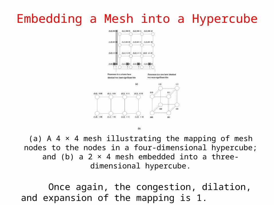
(a) A 4 × 4 mesh illustrating the mapping of mesh nodes to the nodes in a four-dimensional hypercube; and (b) a 2 × 4 mesh embedded into
a three-dimensional hypercube.
Once again, the congestion, dilation, and expansion of the mapping is 1.
Embedding a Mesh into a Linear Array
• Since a mesh has more edges than a linear array, we will not have an optimal congestion/dilation mapping.
• We first examine the mapping of a linear array into a mesh and then invert this mapping.
• This gives us an optimal mapping (in terms of congestion).
Embedding a Mesh into a Linear Array: Example
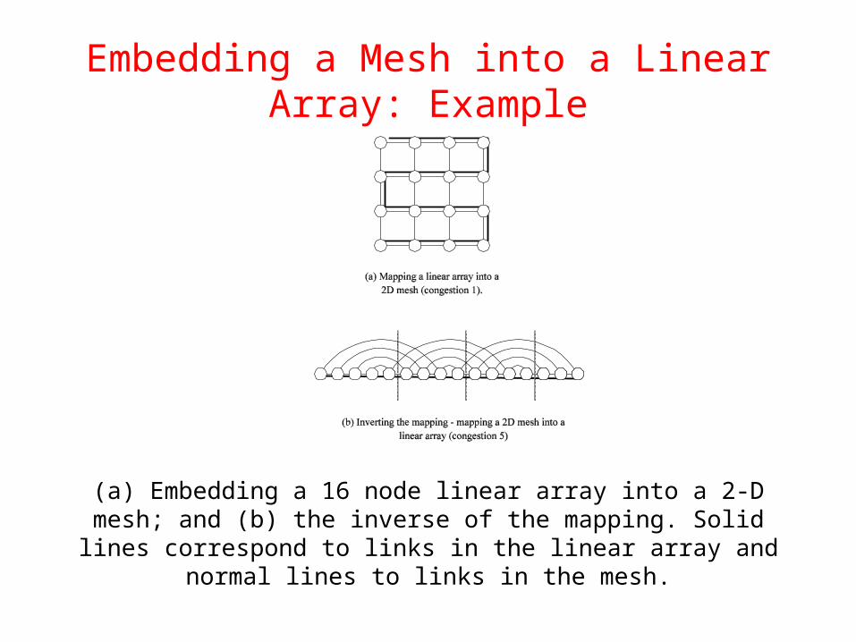
(a) Embedding a 16 node linear array into a 2-D mesh; and (b) the inverse of the mapping. Solid lines correspond to links in the linear
array and normal lines to links in the mesh.
Embedding a Hypercube into a 2-D Mesh
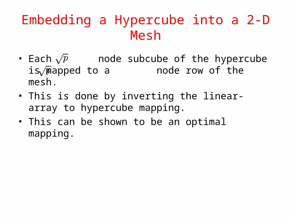
• Each node subcube of the hypercube is mapped to a node row of the mesh.
• This is done by inverting the linear-array to hypercube mapping.
• This can be shown to be an optimal mapping.
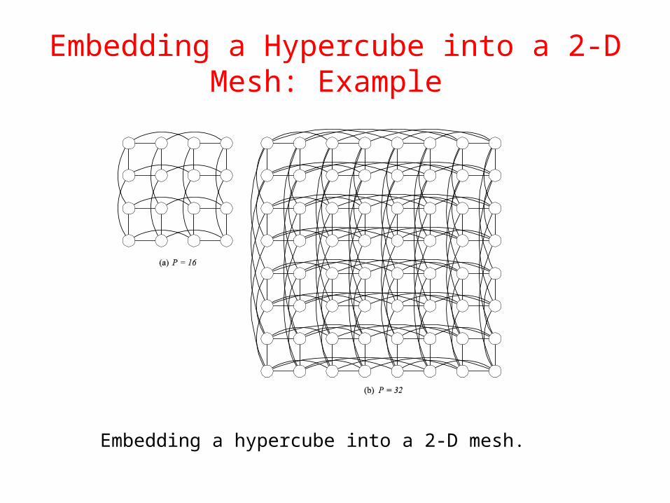
Embedding a Hypercube into a 2-D Mesh: Example
Embedding a hypercube into a 2-D mesh.
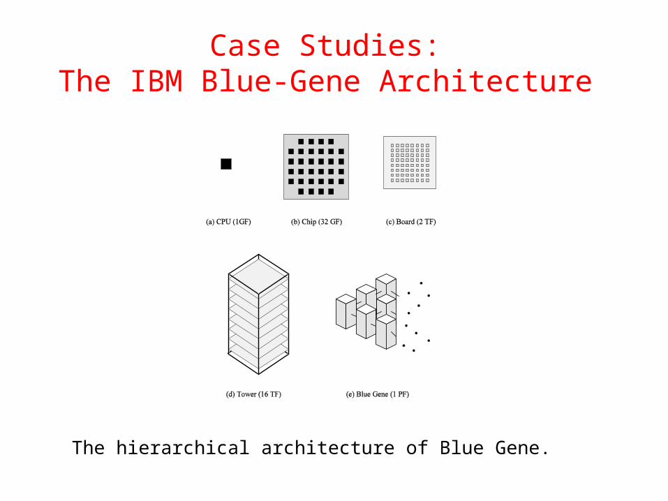
Case Studies: The IBM Blue-Gene Architecture
The hierarchical architecture of Blue Gene.
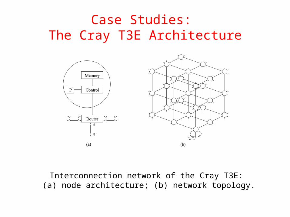
Case Studies: The Cray T3E Architecture
Interconnection network of the Cray T3E: (a) node architecture; (b) network topology.
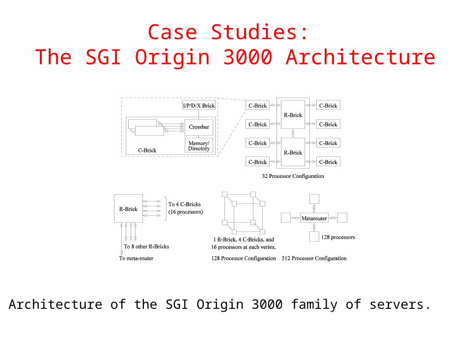
Case Studies: The SGI Origin 3000 Architecture
Architecture of the SGI Origin 3000 family of servers.
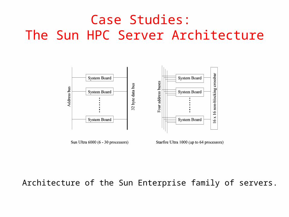
Case Studies: The Sun HPC Server Architecture
Architecture of the Sun Enterprise family of servers.


