Chapter 18. Process Control 18. INTRODUCTION The mathematical models described in previous chapters serve adequately for successful configuration and implementation of unit processes as well as distributed and complex processes. The basic premise in the applications of these models has been that the operation was under steady state conditions. In actual practice however, the steady state condition is easily disturbed by changes in operation variables when the mathematical models are affected. If an ideal steady state condition was taken as the mean of the variations and the deviation from the mean determined, then with proper instrumentation it may be possible to return to steady state operation. Over the years, suitable instruments have been devised for the purpose. They are activated by electric signals generated by individual variables. These signals are programmed to recognize the deviation from the mean. They then suitably operate to restore normal conditions. The main objective for process control therefore is to establish a dynamic mathematical model, monitor the deviation from the model and finally restore the original conditions of operation. The process of controlling a dynamic system is complicated especially in mineral processing systems where a number of variables are involved simultaneously. Developments towards automatic control of plant operations have been commensurate with the development of computer science and instrument technology. Its implementation has resulted in consistent plant performance with improved yield and grade of the product with less manpower. The term "process control" therefore refers to an engineering practice that is directed to the collection of devices and equipment to control processes and systems. Computers find application in simple systems, such as single loop controllers and also in large systems as the Direct Digital Controller (DDC), Supervisory control systems, Hybrid Control Systems and Supervisory Control and Data Acquisition (SCADA) systems. Further developments in process control are supported by many secondary concepts such as computer aided Engineering (CAE). The commonly used present system is the Distributed Control System (DCS). It is made up of three main components, the data highway, the operator station and the microprocessor based controllers. The data highway handles information flow between components ensuring effective communication. The microprocessor controllers are responsible for effective control of the processes and are configured to handle as single or multi-loop controllers. The operator station allows the control command to be given, maintain the system data base and display the process information. The displays normally used are the group and detail displays, trend displays and alarm annunciated displays. In this chapter we will primarily discuss how mathematical models with appropriate instrumentation are used for controlling the quality and quantity of yield of a mineral processing operation.
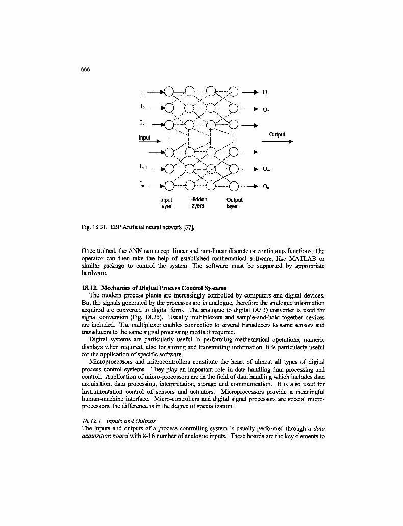
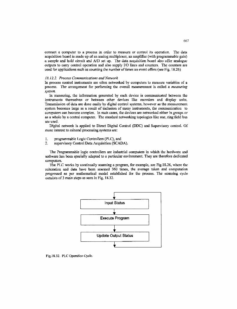
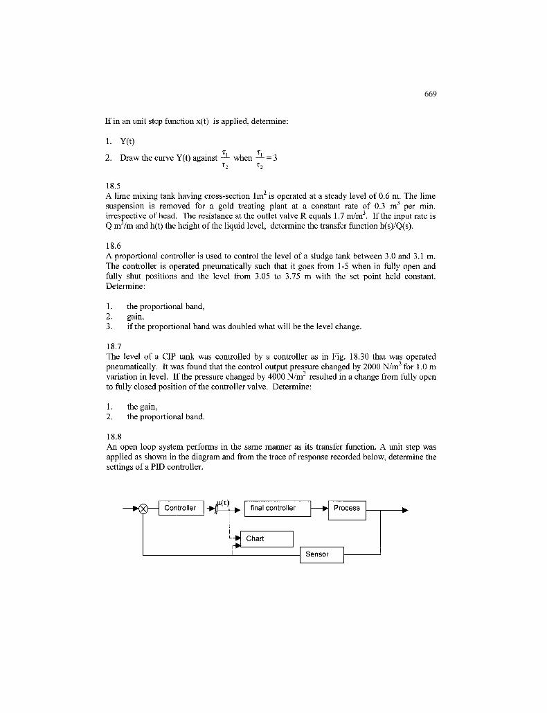
Transcript
Chapter 18. Process Control
18. INTRODUCTION
The mathematical models described in previous chapters serve adequately for successfulconfiguration and implementation of unit processes as well as distributed and complexprocesses. The basic premise in the applications of these models has been that the operationwas under steady state conditions. In actual practice however, the steady state condition iseasily disturbed by changes in operation variables when the mathematical models areaffected. If an ideal steady state condition was taken as the mean of the variations and thedeviation from the mean determined, then with proper instrumentation it may be possible toreturn to steady state operation. Over the years, suitable instruments have been devised for thepurpose. They are activated by electric signals generated by individual variables. Thesesignals are programmed to recognize the deviation from the mean. They then suitably operateto restore normal conditions. The main objective for process control therefore is to establish adynamic mathematical model, monitor the deviation from the model and finally restore theoriginal conditions of operation.
The process of controlling a dynamic system is complicated especially in mineralprocessing systems where a number of variables are involved simultaneously. Developmentstowards automatic control of plant operations have been commensurate with the developmentof computer science and instrument technology. Its implementation has resulted in consistentplant performance with improved yield and grade of the product with less manpower.
The term "process control" therefore refers to an engineering practice that is directed to thecollection of devices and equipment to control processes and systems. Computers findapplication in simple systems, such as single loop controllers and also in large systems as theDirect Digital Controller (DDC), Supervisory control systems, Hybrid Control Systems andSupervisory Control and Data Acquisition (SCADA) systems. Further developments inprocess control are supported by many secondary concepts such as computer aidedEngineering (CAE).
The commonly used present system is the Distributed Control System (DCS). It is madeup of three main components, the data highway, the operator station and the microprocessorbased controllers. The data highway handles information flow between components ensuringeffective communication. The microprocessor controllers are responsible for effective controlof the processes and are configured to handle as single or multi-loop controllers. The operatorstation allows the control command to be given, maintain the system data base and display theprocess information. The displays normally used are the group and detail displays, trenddisplays and alarm annunciated displays.
In this chapter we will primarily discuss how mathematical models with appropriateinstrumentation are used for controlling the quality and quantity of yield of a mineralprocessing operation.
623
Time
Sig
nal
Mean level
623
18.1. Controller Modes
Process control systems can be divided into two major groups:
1. Continuous control that involve monitoring and controlling of events continuously,2 Digital controls that involve the use of computers and microprocessors.
In this book the continuous control system is dealt with more as it forms the basis of thepresent digital system.
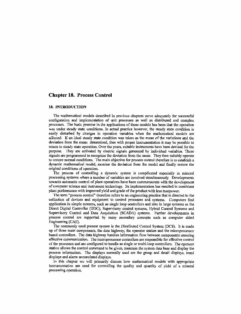
Controlling, say the level of a flotation tank which is being filled continuously and fromwhich the pulp is withdrawn continuously, can be done crudely by observing the rise (or fall)of level and restoring it manually by manipulating valves and increasing or decreasing theinput flow rate to the tank. Such an on-off method would result in an unsteady profile of level(Fig. 18.1). This situation is unacceptable in most mineral processing circuits. To solve theproblem instruments have been devised and strategies developed to minimize the fluctuationsin level. Automatic controllers have therefore being devised which serve to control flowrates, density of slurries, tank and bin levels, pump operations and almost all unit operationslike crushers, mills, screens, classifiers, thickeners, flotation vessels and material handlingsystems.
The two basic control strategies or modes of these controllers are known as:
1. feed back control system, and2. feed forward control system.
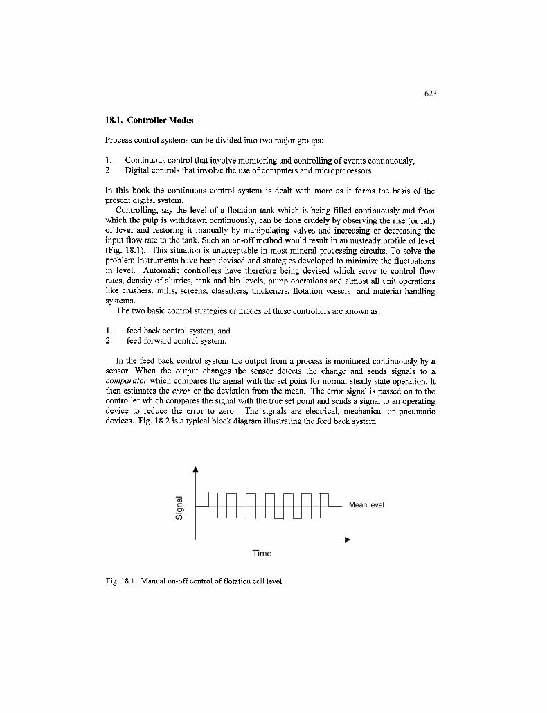
In the feed back control system the output from a process is monitored continuously by asensor. When the output changes the sensor detects the change and sends signals to acomparator which compares the signal with the set point for normal steady state operation. Itthen estimates the error or the deviation from the mean. The error signal is passed on to thecontroller which compares the signal with the true set point and sends a signal to an operatingdevice to reduce the error to zero. The signals are electrical, mechanical or pneumaticdevices. Fig. 18.2 is a typical block diagram illustrating the feed back system
Mean level
Time
Fig. 18.1. Manual on-off control of flotation cell level.
624624
Set point
Comparator
Final controller
", e ^ Controller
>Qpt Feed
^ Process . Output
Sensor
Fig. 18.2. Block diagram of Feed Back control system.
It can be seen that the comparator has three functions. Its first function is to correctlyreceive signals of measured value from the signal monitor. Its second function is to comparethe signal with the set point and then compute the deviation against the norm (set point) andits third function is to activate the final controller to correct the error.
There are two process factors that make the feed back control unsatisfactory. These are theoccurrence of frequent disturbances, often of large magnitude, and the lag time within theprocess between occurrence of an event and delay in recognizing the signal. As shown later,these disturbances and lag times can be measured and corrective steps applied.
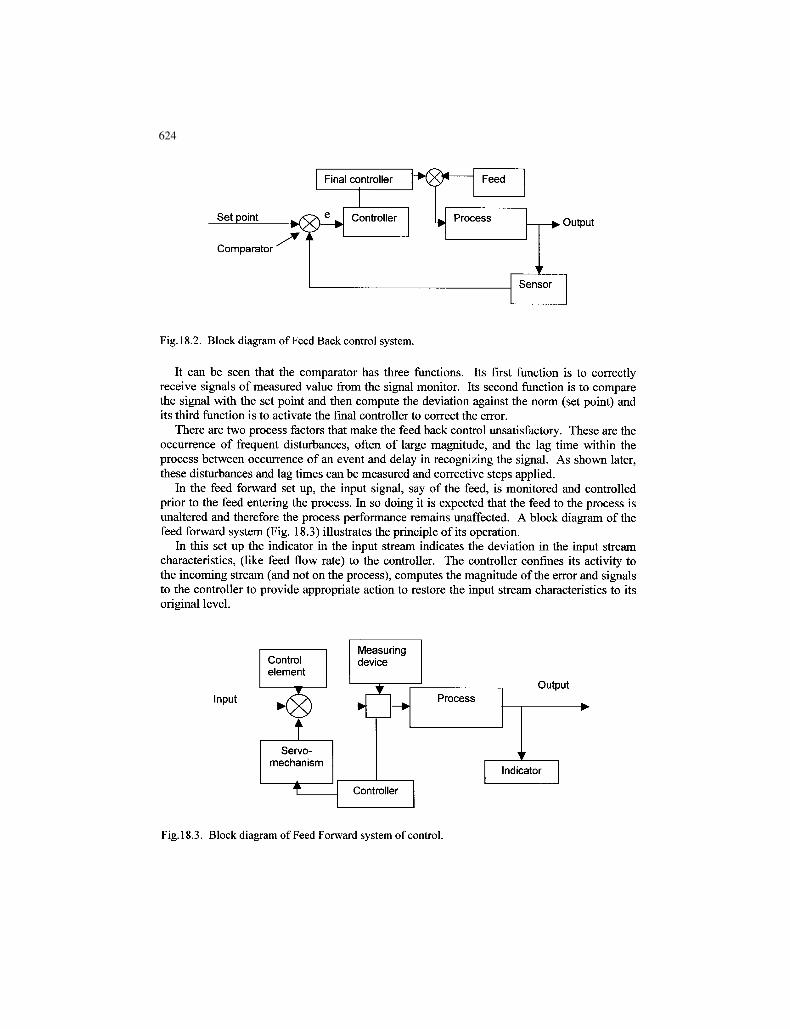
In the feed forward set up, the input signal, say of the feed, is monitored and controlledprior to the feed entering the process. In so doing it is expected that the feed to the process isunaltered and therefore the process performance remains unaffected. A block diagram of thefeed forward system (Fig. 18.3) illustrates the principle of its operation.
In this set up the indicator in the input stream indicates the deviation in the input streamcharacteristics, (like feed flow rate) to the controller. The controller confines its activity tothe incoming stream (and not on the process), computes the magnitude of the error and signalsto the controller to provide appropriate action to restore the input stream characteristics to itsoriginal level.
Input
Controlelement
Measuringdevice
tServo-
mechanism
t
T- •
Process
Controller
Dutnut
r
Indicator
Fig. 18.3. Block diagram of Feed Forward system of control.
625625
Controllers are designed so that the output signal is:
1. proportional to the error2. proportional to the integral of the error,3. proportional to the derivative of the error,4. proportional to a combination of the modes.
When the output signal O, is proportional to the error e, it is known as proportionalcontroller. Mathematically the control action is expressed as:
O = GPe (18.1)
where Gp is the proportionality constant and e the error. Gp is usually known as the gain.
It can be seen that the gain is the ratio of the fractional change in the ratio of the output toinput signals. When e = 0, the output signal is also equal to 0. That is, no signal is emittedfrom the monitor. In this situation Eq. (18.1) is written as:
O = OO + GPe (18.2)
The proportional operation is expressed as proportional band. The band width is the errorto cause 100% change on the metering gauge or chart.
The integral controllers are known as reset controllers. They are so designed that theoutput is proportional to the time integral of the error. Thus the output signal, O, is given by:
O = Gi \e.dt (18.3)o
where Gi is a constant. For integral mode the reset action is more gradual than theproportional controllers.
The derivative mode of controllers stabilizes a process and the controller occupies anintermediate position. An example would be the monitoring of bubbling fluid level whereonly the average fluid level is measured and monitored, like the level in a flotation cell. Theoutput signal in the derivative mode is expressed as:
O = G D ^ (18.4)at
where GD is the constant.
In practice, the proportional mode is usually combined with integral or derivative modesbut most of the time all the three modes are combined. In each combination the output is anadditive function, that is for:
1. For proportional and integral (P+I) mode:
O = O o + G P e + G i |e.<# (18.5)
626
-1
0
1
2
3
4
5
01.5 3 4.5 6 7.5 9
10.5 12 13
.5
Time,secs.
Def
lect
ion
P+D
P
P+IP+I+D
Off set
626
For proportional +derivative (P+D) mode:
'de"= O0+GPe +GD dt
(18.6)
3. For proportional +integral +derivative ( P+I+D) mode:
O = Oo + GP e + Gi f e.dt + GD( —* {dt
(18.7)
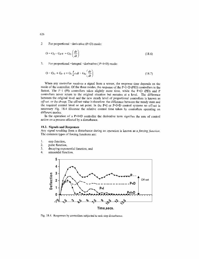
When any controller receives a signal from a sensor, the response time depends on themode of the controller. Of the three modes, the response of the P+I+D (PID) controllers is thefastest. The P+I (PI) controllers takes slightly more time, while the P+D (PD) and Pcontrollers never return to the original situation but remains at a level. The differencebetween the original level and the new steady level of proportional controllers is known asoff-set, or the droop. The off-set value is therefore the difference between the steady state andthe required control level or set point. In the P+I or P+I+D control systems no off-set isnecessary Fig. 18.4 illustrate the relative control time taken by controllers operating ondifferent modes.
In the operation of a P+I+D controller the derivative term signifies the rate of controlaction on a process affected by a disturbance.
18.2. Signals and ResponsesAny signal resulting from a disturbance during an operation is known as a forcing function.The common types of forcing functions are:
Fig. 18.4. Responses by controllers subjected to unit step disturbance.
627
ƒ(t)
0 1 Time, t
X
ƒ(t)
X
Time ,t.
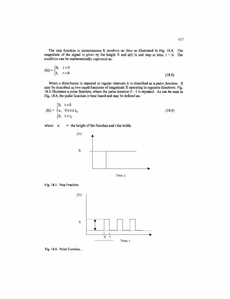
The step function is instantaneous It involves no time as illustrated in Fig. 18.4.magnitude of the signal is given by the height X and u(t) is unit step at time, t = 0.condition can be mathematically expressed as:
627
TheThe
(18.8)
When a disturbance is repeated at regular intervals it is described as a pulse function. Itmay be described as two equal functions of magnitude X operating in opposite directions. Fig.18.6 illustrates a pulse function, where the pulse duration 0 -1 is repeated. As can be seen inFig. 18.6, the pulse function is time based and may be defined as:
fO, t<0/(t)= x, 0<t<t0 (18.9)
where x = the height of the function and t the width.
/(t)
X
Time ,t.
Fig. 18.5. Step Function.
J L0 1
Time, t
Fig. 18.6. Pulse Function.
628
00.10.20.30.40.50.60.70.80.9
1
0 1 2 3 4 5
Time, t
f(t)
-1.5
-1
-0.5
0
0.5
1
1.5
1
1.4
1.8
2.2
2.6 3
3.4
3.8
4.2
4.6 5
5.4
5.8
6.2
6.6
7.5
time,t
f(t)
628
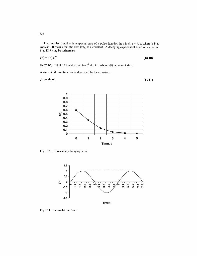
The impulse function is a special case of a pulse function in which x = k/to, where k is aconstant. It means that the area (x to) is a constant. A decaying exponential function shown inFig. 18.7 may be written as:
/(t) = x(t)e"st (18.10)
Here: /(t) = 0 at t < 1 and equal to e"st at t > 0 where x(t) is the unit step.
A sinusoidal time function is described by the equation:
/(t) = sincot (18.11)
10.90.80.70.60.50.40.30.20.1
0
Time, t
Fig. 18.7. Exponentially decaying curve.
1.5-
1 -
0.5-
0
-0.5-
-1 -
-1.5-
N IDIO IO <D <D
time,t
Fig. 18.8. Sinusoidal function.
629629
and its properties are:
f 0, t < 0,/ ( t ) H (18.12)
[xsincot, t > 0
A sinusoidal time function is illustrated in Fig. 18.8. Forcing functions are generallyrepresented by first or second order differential equations. That is:
Aoy =X(t) Zero Order (18.13)
i ^ i + Aoy =X(t) First order (18.14)dx
^ll. + Ai ^ + Aoy = X(t) Second order (18.15)dx dx
where X = input variable or input function andY = output variable, Ao, Ai and A2 are the constants.
For convenience of mathematical manipulations in control systems, Eqs. (18.13) - (18.15)are written in the form of Laplace transforms. On integration the time domain is obviouslyeliminated and a dummy operator is introduced. Thus, sequentially, the three equationstransforms to:
Y(s)= l ( 1 8 1 6 )
(18.17)
(18.18)
Y(s)X(s)
Y(s)X(s)
- 1
1(ra + 1)
1T1S + T1SX2S + T2S
1(T I S + 1)(T2SS + 1
where s is the Laplace dummy operator and T the time constant.
The advantage of using such a technique is that the transforms can be added and subtractedby simple algebraic rules. After the operation the result may be inverted back to time domain(like taking logs and anti-logs of numbers). Derivation of the equations are explained inAppendix C.
18.3. Input and Output Signals of ControllersThe relation between the output and input signals of controllers is conveniently expressed bythe ratio of the output and inputs transforms. The ratio of the transforms is known as thetransfer function. In this book this is referred as TF. The transfer functions of differentmodes of control systems can be easily determined. Where the error is e and Gp, the gain andT the time, the transfer functions of different control modes are given in Table 18.1.
630630
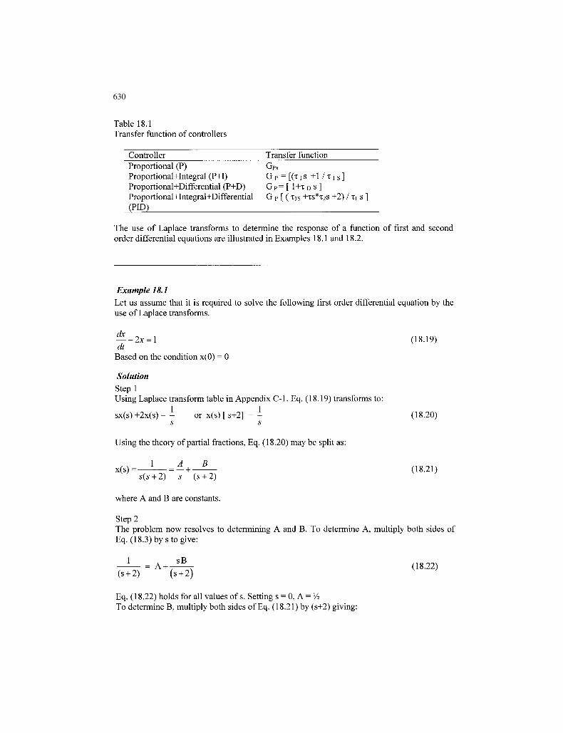
Table 18.1Transfer function of controllers
Controller Transfer functionProportional (P) Gpx
Proportional+Integral (P+I) G P = [(T i s +1 / x i s ]Proportional+Differential (P+D) G P = [ 1+x D s ]Proportional+Integral+Differential G p [ (iis +TS*T2S +2) / TI s ](PIP)
The use of Laplace transforms to determine the response of a function of first and secondorder differential equations are illustrated in Examples 18.1 and 18.2.
Example 18.1Let us assume that it is required to solve the following first order differential equation by theuse of Laplace transforms.
dx— + 2x = l (18.19)dt
Based on the condition x(0) = 0SolutionStep 1Using Laplace transform table in Appendix C-l, Eq. (18.19) transforms to:
sx(s) +2x(s) = - or x(s) [ s+2] = - (18.20)s s
Using the theory of partial fractions, Eq. (18.20) may be split as:
x(s)= = - + — — (18.21)s(s + 2) s (s + 2)
where A and B are constants.
Step 2The problem now resolves to determining A and B. To determine A, multiply both sides ofEq. (18.3) by s to give:
1 A ^ (18-22)(s + 2) (s + 2)
Eq. (18.22) holds for all values of s. Setting s = 0, A = V2
To determine B, multiply both sides of Eq. (18.21) by (s+2) giving:
631631
s s
Eq. (18.23) is true for all values of s, Setting s = -2, B = -V4. Thus Eq. (18.21) converts to:
2s 2
This inverted to time domain gives:
x(t) = 0.5e"°5t (18.25)
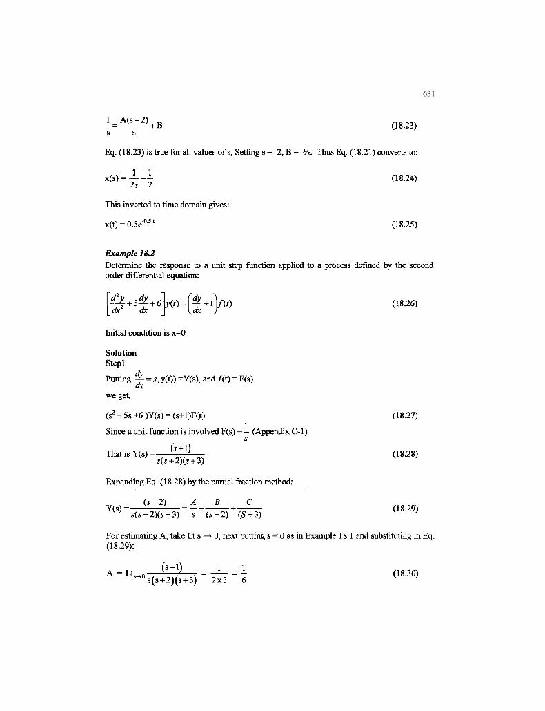
Example 1S.2Determine the response to a unit step function applied to a process defined by the secondorder differential equation:
Initial condition is x=0
SolutionStepl
Putting ^ = s, y(t)) =Y(s), and /(t) = F(s)ax
we get,
(s2+5s+6)Y(s) = (s+l)F(s) (18.27)
Since a unit function is involved F(s) =— (Appendix C-l)s
ThatisY(S) = fr*1) (18.28)( + 2)( + 3)
Expanding Eq. (18.28) by the partial fraction method:
( 1 8 - 2 9 )
For estimating A, take Lt s —* 0, next putting s = 0 as in Example 18.1 and substituting in Eq.(18.29):
A = L t (s + 1) 1 1 (1830)s(s + 2)(s + 3) 2x3 6
632632
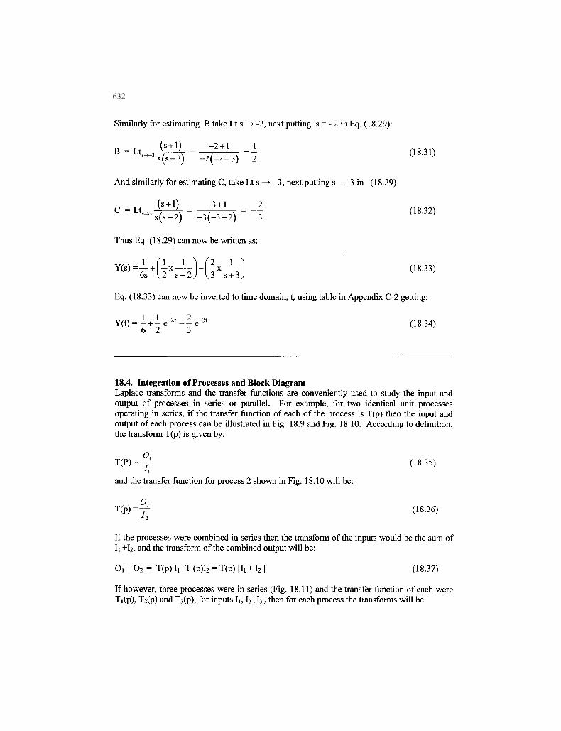
Similarly for estimating B take Lt s —> -2, next putting s = - 2 in Eq. (18.29):
(s + 1) -2 + 1 1B = L t _ 2 4 ^ = — . , = - (18.31)
s ^ 2 s ( s + 3) -2( -2 + 3) 2 V '
And similarly for estimating C, take Lt s —> - 3, next putting s = - 3 in (18.29)
C=Lt fr±*U 2 + \=-l (18.32)~ 3 s ( s + 2) -3(-3 + 2) 3 V ;
Thus Eq. (18.29) can now be written as:
Y(s)=—+ - x - ^ - - - x - = - (18.33)6s U s + 2j U s + 3j
Eq. (18.33) can now be inverted to time domain, t, using table in Appendix C-2 getting:
Y(t) = - + - e"2t - - e"3t (18.34)6 2 3 K '
18.4. Integration of Processes and Block DiagramLaplace transforms and the transfer functions are conveniently used to study the input andoutput of processes in series or parallel. For example, for two identical unit processesoperating in series, if the transfer function of each of the process is T(p) then the input andoutput of each process can be illustrated in Fig. 18.9 and Fig. 18.10. According to definition,the transform T(p) is given by:
T (P )=y - (18.35)
and the transfer function for process 2 shown in Fig. 18.10 will be:
T(p)=~ (18.36)
If the processes were combined in series then the transform of the inputs would be the sum ofIi +I2, and the transform of the combined output will be:
If however, three processes were in series (Fig. 18.11) and the transfer function of each wereTi(p), T2(p) and Ts(p), for inputs Ii, I2,13, then for each process the transforms will be:
633633
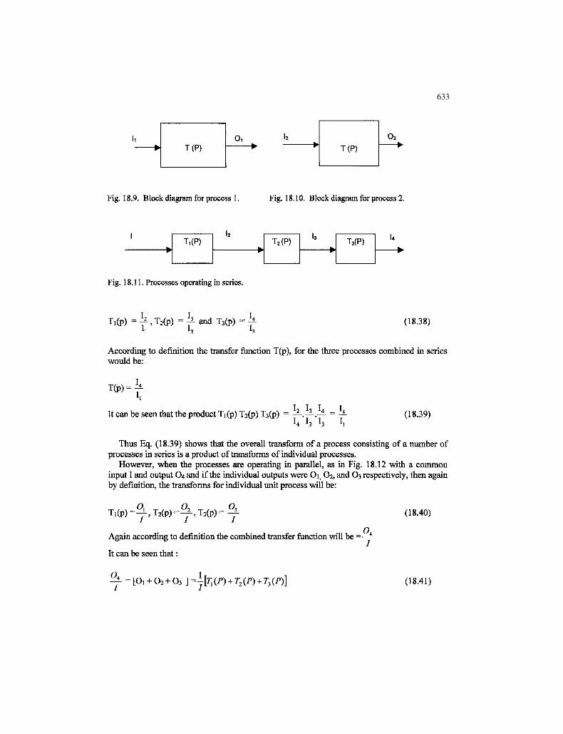
Fig. 18.9. Block diagram for process 1. Fig. 18.10. Block diagram for process 2.
Ti(P) T2(P) T3(P)
Fig. 18.11. Processes operating in series.
Ti(p) = f, T2(p) = i . ^ T3(p) = f (18.38)
According to definition the transfer function T(p), for the three processes combined in serieswould be:
It can be seen that the product Ti(p) T2(p) T3(p) = —.—.— = -*-I4 I2 I3 I,
(18.39)
Thus Eq. (18.39) shows that the overall transform of a process consisting of a number ofprocesses in series is a product of transforms of individual processes.
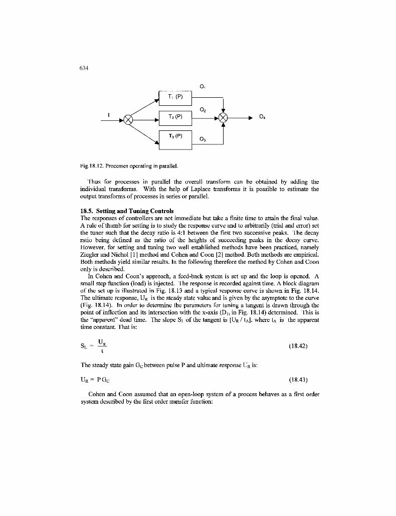
However, when the processes are operating in parallel, as in Fig. 18.12 with a commoninput I and output O4 and if the individual outputs were Oi, O2, and O3 respectively, then againby definition, the transforms for individual unit process will be:
(18.40)
Again according to definition the combined transfer function will be =—-
It can be seen that:
l[Tl (18.41)
634634
Fig.18.12. Processes operating in parallel.
Thus for processes in parallel the overall transform can be obtained by adding theindividual transforms. With the help of Laplace transforms it is possible to estimate theoutput transforms of processes in series or parallel.
18.5. Setting and Tuning ControlsThe responses of controllers are not immediate but take a finite time to attain the final value.A rule of thumb for setting is to study the response curve and to arbitrarily (trial and error) setthe tuner such that the decay ratio is 4:1 between the first two successive peaks. The decayratio being defined as the ratio of the heights of succeeding peaks in the decay curve.However, for setting and tuning two well established methods have been practiced, namelyZiegler and Nichol [1] method and Cohen and Coon [2] method. Both methods are empirical.Both methods yield similar results. In the following therefore the method by Cohen and Coononly is described.
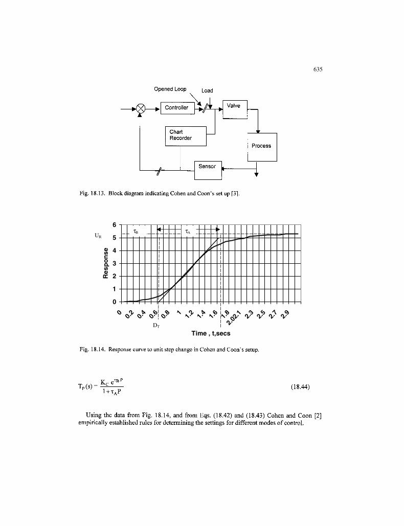
In Cohen and Coon's approach, a feed-back system is set up and the loop is opened. Asmall step function (load) is injected. The response is recorded against time. A block diagramof the set up is illustrated in Fig. 18.13 and a typical response curve is shown in Fig. 18.14.The ultimate response, UR is the steady state value and is given by the asymptote to the curve(Fig. 18.14). In order to determine the parameters for tuning a tangent is drawn through thepoint of inflection and its intersection with the x-axis (D-n in Fig. 18.14) determined. This isthe "apparent" dead time. The slope SL of the tangent is [UR/ tA]. where tA is the apparenttime constant. That is:
s, = t
The steady state gain Gc between pulse P and ultimate response UR is:
UR= PGC
(18.42)
(18.43)
Cohen and Coon assumed that an open-loop system of a process behaves as a first ordersystem described by the first order transfer function:
635
0
1
2
3
4
5
6
0 0.2
0.4
0.6
0.8 1 1.
21.
41.
61.
8
2.02
.1 2.3
2.5
2.7
2.9
Time , t,secs
Res
po
nse
UR τB τA
DT
635
Opened Loop L o a c |
Controller
ChartRecorder
Sensor
Valve
r
Process
Fig. 18.13. Block diagram indicating Cohen and Coon's set up [3].
O -
5 -
8 4-
10
£ 2-1 -
n -
_. . % _
**•
D
I
<
r
/
\
XA
/
A
/
>f >
•P*- - • —
c
Time, t,secs
Fig. 18.14. Response curve to unit step change in Cohen and Coon's setup.
T (z) -p ( )
(18.44)
Using the data from Fig. 18.14, and from Eqs. (18.42) and (18.43) Cohen and Coon [2]empirically established rules for determining the settings for different modes of control.
636636
The empirical method designed by Cohen and Coon (and also Ziegler and Nichols), arebeing increasingly replaced by the "model methods" of tuning [4,5,7]. Two such modelmethods presently used are:
1. ITAE (Integral Time weight absolute error),2. IMC (Internal model control).
The ITAE method arises from the fact that the decay ratio of 4:1 for the first two peaks isnot necessarily the same for the subsequent peaks. Thus an error is introduced. Tominimizing this error, the process is considered as first order with a time delay. The output-input ratio is given by the transfer function:
O ^ = G p ^ ( i g 4 5 )
Is xPs + l
where Os = Output of process,Is = Input to process,Gp = Process gain,XD = Process t ime delay,
xp = Process t ime constant
xc = Closed loop t ime constantIs = Input to process (Controller output)
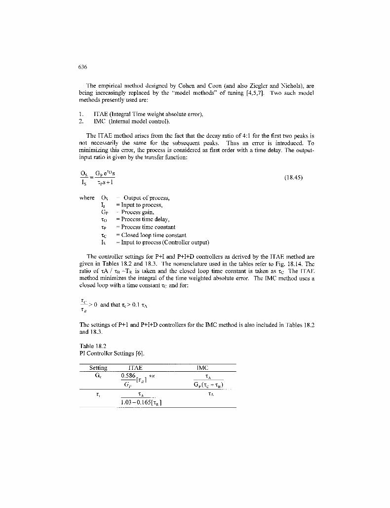
The controller settings for P+I and P+I+D controllers as derived by the ITAE method aregiven in Tables 18.2 and 18.3. The nomenclature used in the tables refer to Fig. 18.14. Theratio of xA / TB = T R . is taken and the closed loop time constant is taken as xc The ITAEmethod minimizes the integral of the t ime weighted absolute error. The IMC method uses aclosed loop with a t ime constant xc and for:
— > 0 and that x c > 0.1 xA
The settings of P+1 and P+I+D controllers for the IMC method is also included in Tables 18.2and 18.3.
Table 18.2PI Controller Settings [6].
Setting
Gc
T,
0
1
ITAE
.586 9i6
GP *R
xA
.03-0.165 [xR ]
IMC
GP(TC + xB)
637637
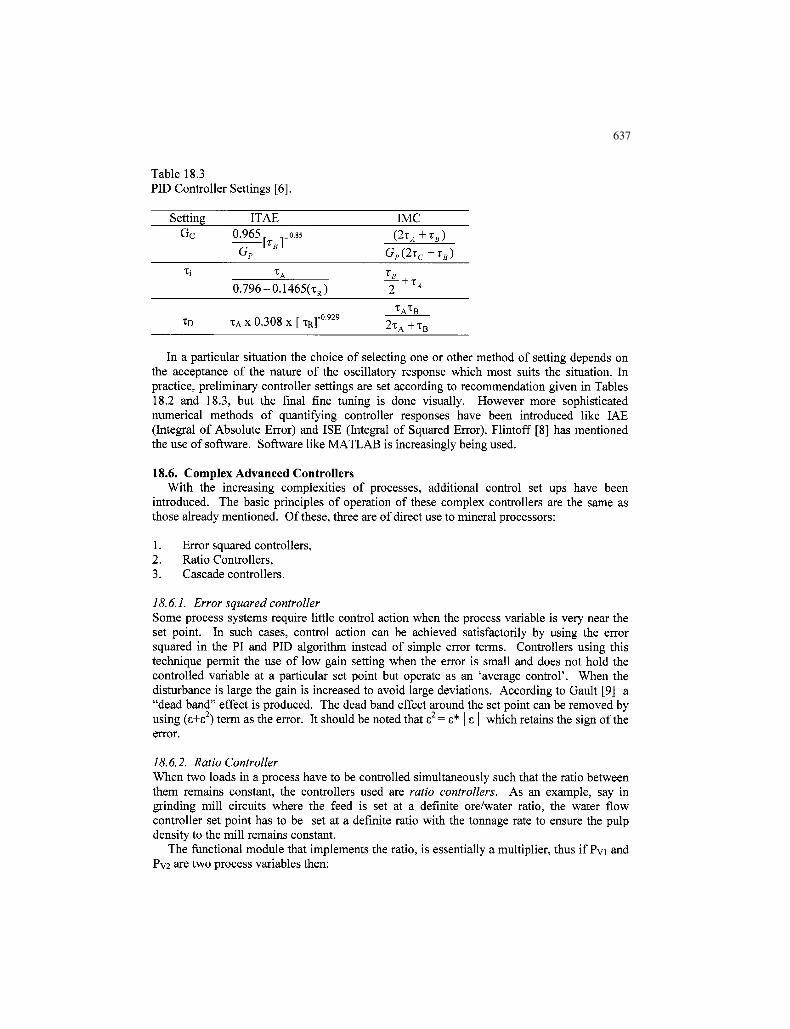
Table 18.3PID Controller
SettingGc
Ti
XD
Settings [6].
ITAE0.965 0.85
GP [TR1
TA
0.796-0.1465(xR)
xAx 0.308 X [ T R ] - 0 9 2 9
(
2
2T
IMC2 T ^ + T B )
>(2r c+rB)
+ T^
C A T B
A+TB
In a particular situation the choice of selecting one or other method of setting depends onthe acceptance of the nature of the oscillatory response which most suits the situation. Inpractice, preliminary controller settings are set according to recommendation given in Tables18.2 and 18.3, but the final fine tuning is done visually. However more sophisticatednumerical methods of quantifying controller responses have been introduced like IAE(Integral of Absolute Error) and ISE (Integral of Squared Error). Flintoff [8] has mentionedthe use of software. Software like MATLAB is increasingly being used.
18.6. Complex Advanced ControllersWith the increasing complexities of processes, additional control set ups have been
introduced. The basic principles of operation of these complex controllers are the same asthose already mentioned. Of these, three are of direct use to mineral processors:
1. Error squared controllers,2. Ratio Controllers,3. Cascade controllers.
18.6.1. Error squared controllerSome process systems require little control action when the process variable is very near theset point. In such cases, control action can be achieved satisfactorily by using the errorsquared in the PI and PID algorithm instead of simple error terms. Controllers using thistechnique permit the use of low gain setting when the error is small and does not hold thecontrolled variable at a particular set point but operate as an 'average control'. When thedisturbance is large the gain is increased to avoid large deviations. According to Gault [9] a"dead band" effect is produced. The dead band effect around the set point can be removed byusing (s+s2) term as the error. It should be noted that e2 = e* | s | which retains the sign of theerror.
18.6.2. Ratio ControllerWhen two loads in a process have to be controlled simultaneously such that the ratio betweenthem remains constant, the controllers used are ratio controllers. As an example, say ingrinding mill circuits where the feed is set at a definite ore/water ratio, the water flowcontroller set point has to be set at a definite ratio with the tonnage rate to ensure the pulpdensity to the mill remains constant.
The functional module that implements the ratio, is essentially a multiplier, thus if PVi andPv2 are two process variables then:
638638
R Pv2 or R = — L (18.46)
R is known as the settable ratio. The ratio station has similar features to the PID system[10].
The prime role of the ratio station is to provide a way of generating the set point. The ratioitself becomes a set point controlled by higher level control in a structured system.
The ratio controllers can be used both in open and closed loops. Such controllers are oftenused in practice in flotation circuits where the water additions is related to the target feedrate and in circuits where pH control is required, say lime additions, in gold cyanidationprocess.
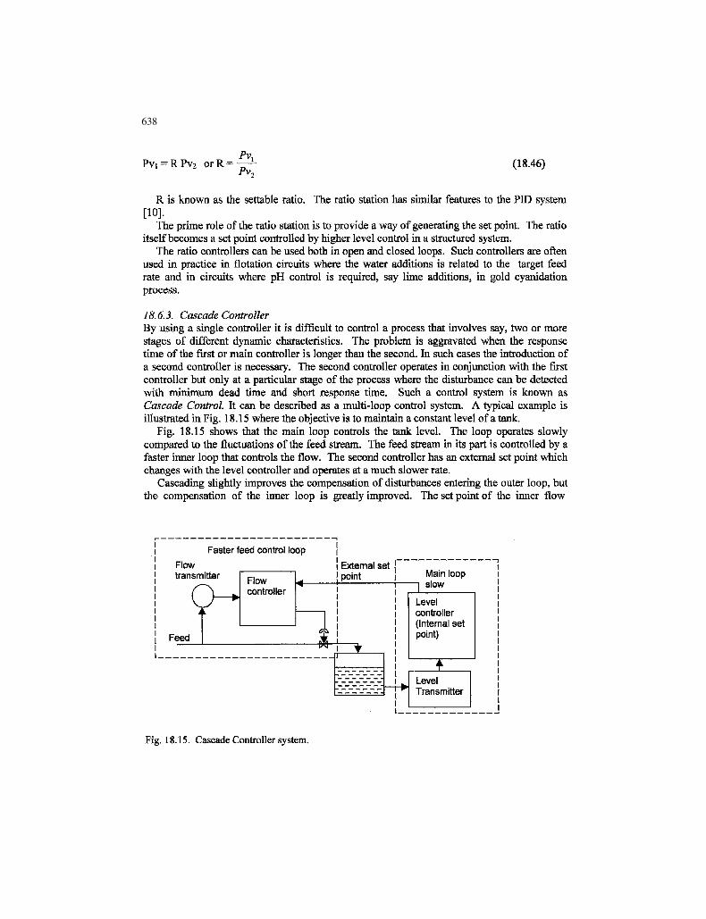
18.6,3. Cascade ControllerBy using a single controller it is difficult to control a process that involves say, two or morestages of different dynamic characteristics. The problem is aggravated when the responsetime of the first or main controller is longer than the second. In such cases the introduction ofa second controller is necessary. The second controller operates in conjunction with the firstcontroller but only at a particular stage of the process where the disturbance can be detectedwith minimum dead time and short response time. Such a control system is known asCascade Control. It can be described as a multi-loop control system. A typical example isillustrated in Fig. 18.15 where the objective is to maintain a constant level of a tank.
Fig. 18.15 shows that the main loop controls the tank level. The loop operates slowlycompared to the fluctuations of the feed stream. The feed stream in its part is controlled by afaster inner loop that controls the flow. The second controller has an external set point whichchanges with the level controller and operates at a much slower rate.
Cascading slightly improves the compensation of disturbances entering the outer loop, butthe compensation of the inner loop is greatly improved. The set point of the inner flow
Faster feed control loopFlowtransmitter
Feed
Flowcontroller
External setpoint Main loop
slow
Levelcontroller(Internal setpoint)
Fig. 18.15. Cascade Controller system.
639639
controller is obtained from the output of the level controller. The cascade control systemprovides a high degree of stabilization to the overall control.
18.6.4. Adaptive ControllerAn adaptive control system automatically compensates for variations in system dynamics byadjusting the controller characteristics so that the overall system performance remains thesame, or rather maintained at optimum level. This control system takes into account anydegradation in plant performance with time. The adaptive control system includes elementsto measure (or estimate) the process dynamics and other elements to alter the controllercharacteristics accordingly. The controller adjusts the controller characteristics in a manner tomaintain the overall system performance. The basic essentials of the adaptive system are:
1. Identification of system dynamics,2. Decision, and3. Modification.
Once the system is identified, (which is a difficult process) the decision function operates.This in turn activates the modification function to alter the particular process parameter and tomaintain optimum performance.
The common ways of evaluating performance are by model comparison and performancecriteria. In the model comparison system, a model is selected that bears resemblance to thedesired system characteristics. In it, all effects of the system characters and effects ofdisturbances are known. According to Gault [9] the response characteristics of the controlsystem variable parameters are "slaved" to the response characteristics of the referencemodel. The error between the model and the control system is acted on. This action isaccomplished by an adaptive operation which produces the required system gains. The pathof adaptation is the minimization of the integral of the error square.
In the performance criterion, a general performance index such as the integral of the errorsquared is chosen and continuously computed. The system is adjusted to keep the value of theindex at a minimum level. A development of this is the Kalmin Filter [7]. This is acomplicated process. Interested readers are referred to the work of Stephanopoulos [11],Flintoff and Mular [12],
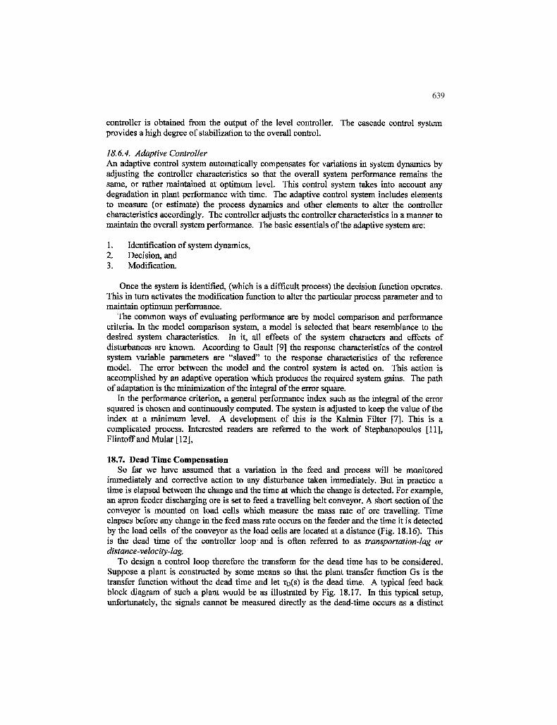
18.7. Dead Time CompensationSo far we have assumed that a variation in the feed and process will be monitored
immediately and corrective action to any disturbance taken immediately. But in practice atime is elapsed between the change and the time at which the change is detected. For example,an apron feeder discharging ore is set to feed a travelling belt conveyor. A short section of theconveyor is mounted on load cells which measure the mass rate of ore travelling. Timeelapses before any change in the feed mass rate occurs on the feeder and the time it is detectedby the load cells of the conveyor as the load cells are located at a distance (Fig. 18.16). Thisis the dead time of the controller loop and is often referred to as transportation-lag ordistance-velocity-lag.
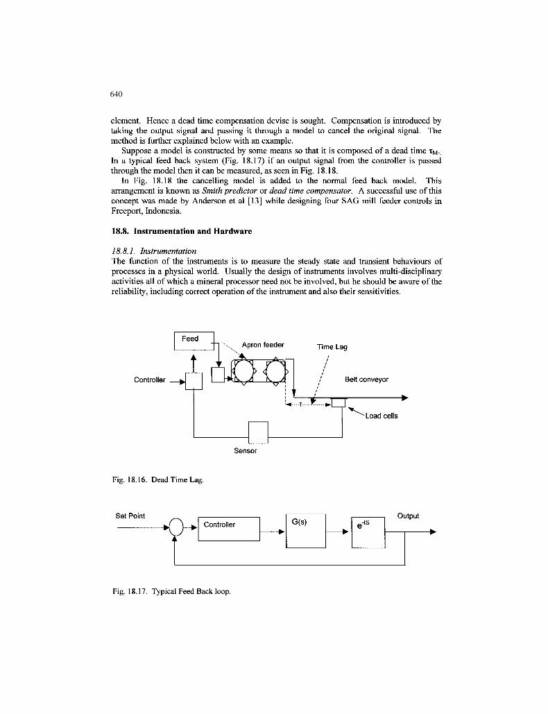
To design a control loop therefore the transform for the dead time has to be considered.Suppose a plant is constructed by some means so that the plant transfer function Gs is thetransfer function without the dead time and let TD(S) is the dead time. A typical feed backblock diagram of such a plant would be as illustrated by Fig. 18,17. In this typical setup,unfortunately, the signals cannot be measured directly as the dead-time occurs as a distinct
640640
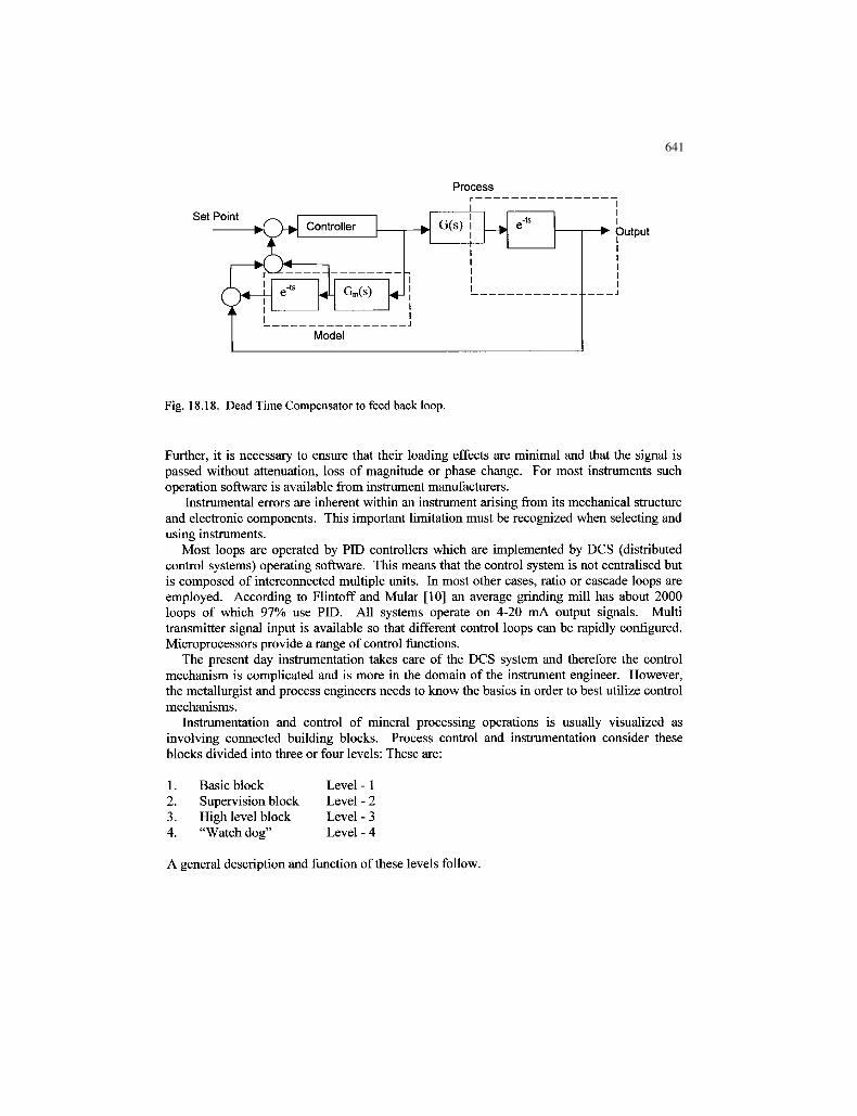
element. Hence a dead time compensation devise is sought. Compensation is introduced bytaking the output signal and passing it through a model to cancel the original signal. Themethod is further explained below with an example.
Suppose a model is constructed by some means so that it is composed of a dead time TM..In a typical feed back system (Fig. 18.17) if an output signal from the controller is passedthrough the model then it can be measured, as seen in Fig. 18.18.
In Fig. 18.18 the cancelling model is added to the normal feed back model. Thisarrangement is known as Smith predictor or dead time compensator. A successful use of thisconcept was made by Anderson et al [13] while designing four SAG mill feeder controls inFreeport, Indonesia.
18.8. Instrumentation and Hardware
18.8.1. InstrumentationThe function of the instruments is to measure the steady state and transient behaviours ofprocesses in a physical world. Usually the design of instruments involves multi-disciplinaryactivities all of which a mineral processor need not be involved, but he should be aware of thereliability, including correct operation of the instrument and also their sensitivities.
Controller WJApron feeder Time Lag
Belt conveyor
- Load cells
Sensor
Fig. 18.16. Dead Time Lag.
Set Point rw Controller G(s)
—
Output
Fig. 18.17. Typical Feed Back loop.
641641
Process
Set PointOutput
Fig. 18.18. Dead Time Compensator to feed back loop.
Further, it is necessary to ensure that their loading effects are minimal and that the signal ispassed without attenuation, loss of magnitude or phase change. For most instruments suchoperation software is available from instrument manufacturers.
Instrumental errors are inherent within an instrument arising from its mechanical structureand electronic components. This important limitation must be recognized when selecting andusing instruments.
Most loops are operated by PID controllers which are implemented by DCS (distributedcontrol systems) operating software. This means that the control system is not centralised butis composed of interconnected multiple units, hi most other cases, ratio or cascade loops areemployed. According to Flintoff and Mular [10] an average grinding mill has about 2000loops of which 97% use PID. All systems operate on 4-20 mA output signals. Multitransmitter signal input is available so that different control loops can be rapidly configured.Microprocessors provide a range of control functions.
The present day instrumentation takes care of the DCS system and therefore the controlmechanism is complicated and is more in the domain of the instrument engineer. However,the metallurgist and process engineers needs to know the basics in order to best utilize controlmechanisms.
Instrumentation and control of mineral processing operations is usually visualized asinvolving connected building blocks. Process control and instrumentation consider theseblocks divided into three or four levels: These are:
A general description and function of these levels follow.
642642
Level 1 controlThis is the regulatory level where basic controls loops like, P+I control loops include controlof feed tonnages from bins, conveyors, manipulating of bins, water addition loop (in millingcircuit) pump speed and sump level controls, thickener overflow density control etc areinvolved (depending on the process circuit).
Level 2This is a supervisory control stage that includes process stabilization and optimizing, usuallyusing cascade loop and ratio loops. For example, in a ball mill circuit the ratio loop controlsthe ball mill water while the cascade loop controls the particle size of product bymanipulating the tonnage set point.
Level 3Controls at this level include maximizing circuit throughput, limiting circulating load (whereapplicable).
Level 4This is a higher degree of supervisory controls of various operations including plant shutdowns for maintenance or emergency. Austin [14] has referred to level 4 controls as "watch-dog" control.
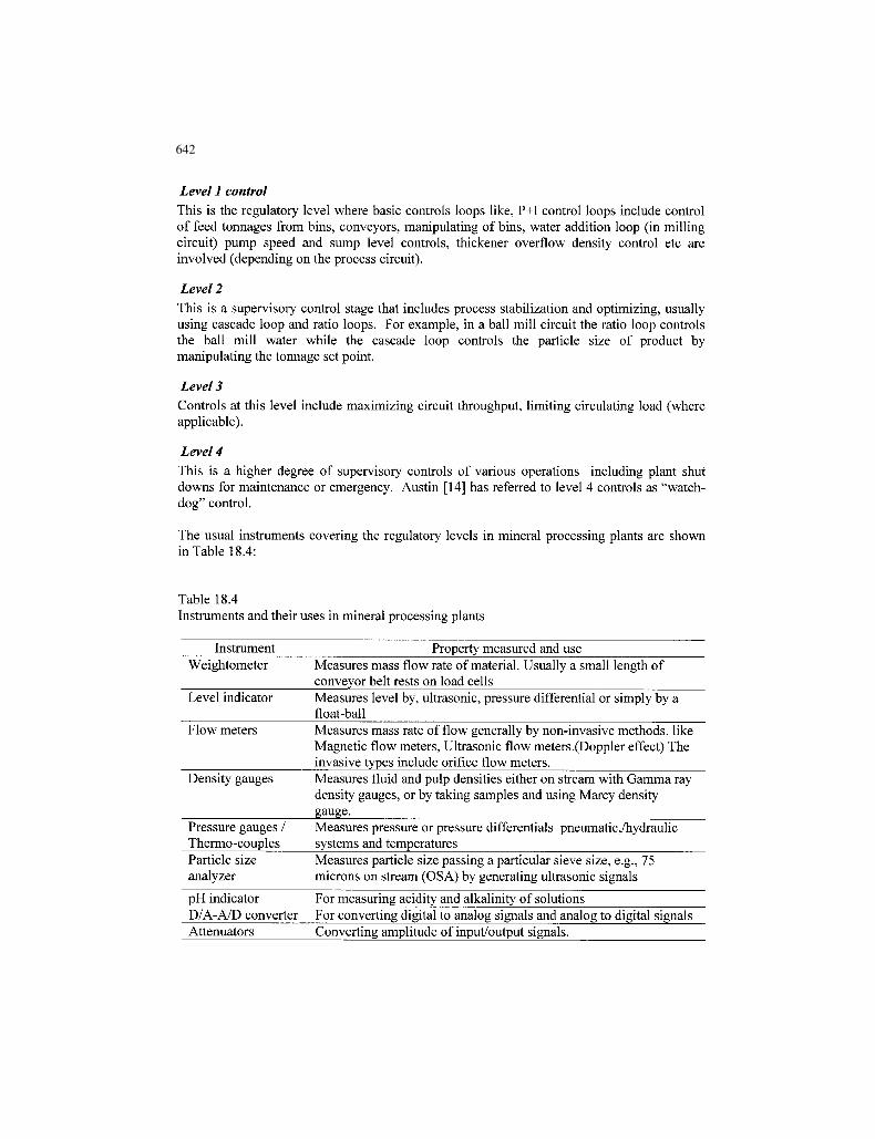
The usual instruments covering the regulatory levels in mineral processing plants are shownin Table 18.4:
Table 18.4Instruments and their uses in mineral processing plants
Instrument Property measured and useWeightometer Measures mass flow rate of material. Usually a small length of
conveyor belt rests on load cellsLevel indicator Measures level by, ultrasonic, pressure differential or simply by a
float-ballFlow meters Measures mass rate of flow generally by non-invasive methods, like
Magnetic flow meters, Ultrasonic flow meters.(Doppler effect) Theinvasive types include orifice flow meters.
Density gauges Measures fluid and pulp densities either on stream with Gamma raydensity gauges, or by taking samples and using Marcy densitygauge.
Pressure gauges / Measures pressure or pressure differentials pneumatic,/hydraulicThermo-couples systems and temperaturesParticle size Measures particle size passing a particular sieve size, e.g., 75analyzer microns on stream (OSA) by generating ultrasonic signals
pH indicator For measuring acidity and alkalinity of solutionsD/A-A/D converter For converting digital to analog signals and analog to digital signalsAttenuators Converting amplitude of input/output signals.
643643
18.8,2. Hardware
Pneumatic ValvesIn mineral processing operations where flow of fluids and slurries are frequently measured, avalve at the inlet and outlet of operation is common. In effect the valve serves as a part of theoperation as distinct from instruments which indicate the status of a particular operatingcondition. In several circuits it forms the final control of the system. Therefore its transformhas to be included in block diagram algebra.
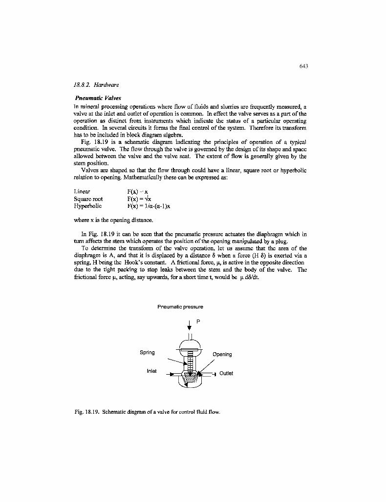
Fig. 18.19 is a schematic diagram indicating the principles of operation of a typicalpneumatic valve. The flow through the valve is governed by the design of its shape and spaceallowed between the valve and the valve seat. The extent of flow is generally given by thestem position.
Valves are shaped so that the flow through could have a linear, square root or hyperbolicrelation to opening. Mathematically these can be expressed as:
F(x) = xF(x) = VF(x) =
LinearSquare rootHyperbolic
where x is the opening distance.
In Fig. 18.19 it can be seen that the pneumatic pressure actuates the diaphragm which inturn affects the stem which operates the position of the opening manipulated by a plug.
To determine the transform of the valve operation, let us assume that the area of thediaphragm is A, and that it is displaced by a distance 5 when a force (H 8) is exerted via aspring, H being the Hook's constant. A factional force, ji, is active in the opposite directiondue to the tight packing to stop leaks between the stem and the body of the valve. Thefrictional force u, acting, say upwards, for a short time t, would be u. ddVdt.
Pneumatic pressure
P
Spring
Inlet -I Outlet
Fig. 18.19. Schematic diagram of a valve for control fluid flow.
644644
Let P be the signal representing the force that opens and closes the valve. Thedisplacement 8 of the valve (diaphragm) is equal to the opposing pressure of the spring.
M d2d ddPA=——r + fi — + HS (18.47)
Dividing by H and transposing,
, i__lz i c _ (]R Afi^
This is a second order differential equation and as we can put:
M 1, , . f =- (18.49)
g ti H 0
The standard transform of this second order system is:
'' - A / H - ^ , + H (18.50)P(s) [M/Hg\ H
The present trend is to invariably use electronically operated actuators instead ofpneumatically operated valves, hi either case the transform will remain unaltered [15].
18.8.3. Other HardwareOther hardware relates to electrical functions (capacitance, resistance, and inductance)mechanical systems like springs, frictional systems, rotational systems and mechanisms tosuit particular setups. Transfer functions of some common selected hardware are given inAppendix C-2.
18.9. Controls of Selected Mineral Processing CircuitsMineral processing operations are dynamic systems. Disturbances arise primarily due to
variations in process inputs and also due to the process machinery both of which combine toaffect the smooth operation of processes. To understand the strategy of process optimizationand control for steady operation let us consider a simple unit operation like the control of thesolid level in bins and hoppers or the fluid level in a tank. The principle underlying thecontrol strategy is the same in both systems while the hardware and operation methods differ.Level control of bins, bunkers and solids storages, are more complicated as the solids in thesevessels are almost never level. For smooth liquid level in tanks, this problem obviously doesnot arise, hi the following section the simpler situation of controlling the fluid level in tanksor similar vessel is examined.
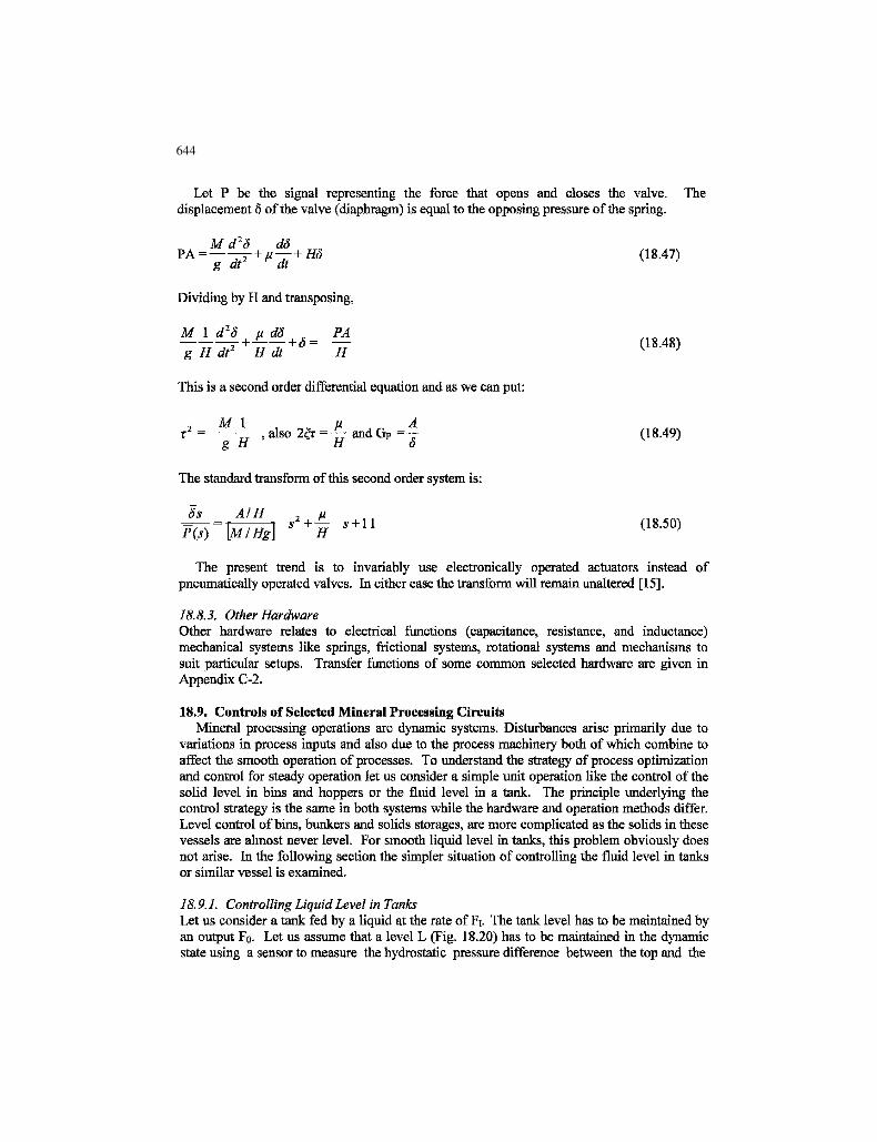
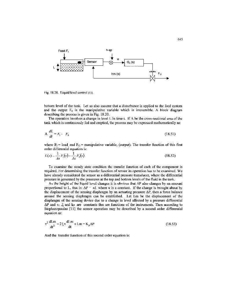
18.9.1. Controlling Liquid Level in TanksLet us consider a tank fed by a liquid at the rate of Fi. The tank level has to be maintained byan output Fo. Let us assume that a level L (Fig. 18.20) has to be maintained in the dynamicstate using a sensor to measure the hydrostatic pressure difference between the top and the
645645
Feed F, h-sp
1Sensor Gc(s)
hm (s)
Fig. 18.20. Liquid level control [11].
bottom level of the tank. Let us also assume that a disturbance is applied to the feed systemand the output Fo is the manipulative variable which is irreversible. A block diagramdescribing the process is given in Fig. 18.20.
The operation involves a change in level L in time t. If A be the cross-sectional area of thetank which is continuously fed and emptied, the process may be expressed mathematically as:
dL(18.51)
where Fi = load and Fo = manipulative variable, (output). The transfer function of this firstorder differential equation is:
As As(18.52)
To examine the steady state condition the transfer function of each of the component isrequired. For determining the transfer function of sensor its operation has to be examined. Wehave already considered the sensor as a differential pressure transducer, where the differentialpressure is generated by the pressures at the top and bottom levels of the fluid in the tank.
As the height of the liquid level changes it is obvious that AP also changes by an amountproportional to L, that is: AP = KL where K is a constant. If the change is brought about bythe displacement of the sensing diaphragm by an actuating pressure AP, then a force balancearound the sensing diaphragm can be established. Let Lm be the displacement of thediaphragm of the sensing device due to a change in level affected by a pressure differentialAP and ti ,£, and kp are constants that are functions of the instruments. Then according toStephanopoulas [11] the sensor operation may be described by a second order differentialequation as:
dLm dLmdt
= KpAP (18.53)
And the transfer function of this second order equation is:
646646
Eq. (18.54) therefore is the transfer function of the sensor.
Let us assume that a P+I controller is used and a set point Lsp is set, Then the transferfunction of the error, e will be:
e =[lsp(s)-Lm(s)] (18.55)
We have seen (Table 18.2) that for a P+I controller whose output is O , the transferfunction is given by:
O(s) = Gc 1 + — e(s) (18.56)
L T s JFor the final control element, that is a control valve, the transfer function of the response is
a first order system and therefore can be written as:
F0(s) = - ^ - c ( s ) (18.57)T+l
From the block diagram it can be seen that the components operate in series. Thus Eq. (1839) applies. In the general case, if Gc(s) is the transfer function of the controller, GF(S), thatof final element, Gp(s), of the process, Gm that of the sensor (measuring device), thenaccording to block diagram algebra the response of the output to the change of set point willbe:
G ( s ) G ( s ) G ( s )
l + Gp(s)GF(s)Gc(s)Gm(s)G ( s ) G ( s ) G ( s )
l + G ( s ) G ( s ) G ( s ) G ( s ) SP
And the effect on output due to a disturbance (change in load) will be:
O, (s) = . . G,Ay . , — x d(s) (18.59)2 W l + G p ( s )G F ( s )G c ( s )G m ( s )
The closed loop response will be the sum of Eqs. (18.58) and (18.59), that is:
— GP(s)GF(s)Gc(s) GH
O (s) = , , F Y , C Y x + T^ 7^ ^ TT x d 0 ) 08-6°)l + GP(s)GF(s)Gc(s)) l + Gp(s)GF(s)Gc(s)Gm(s)
The response in time domain to a change in the level due to a change in load will be givenby the inverse of Eq. (18.60) which would contribute to the control the level of tank.
647647
The principles explained in this simple control system are applicable to all controllingoperations. In integrated unit processes encountered in normal mineral processing operations,the applications become more complicated and would depending on the circuit diagram.
In the following, principle considerations which go to control selected mineral processingoperations are described.
18.9.2. Crushing Plant ControlThe control of any crushing operations starts with the control of the feed system. Lynch [16]has summarized the disturbances in a crusher as:
1. ore properties (size and hardness),2. ore feed rate,3. crusher settings (close and open settings) — alterations due to wear and tear,4. surge in feed load and plant power draw.
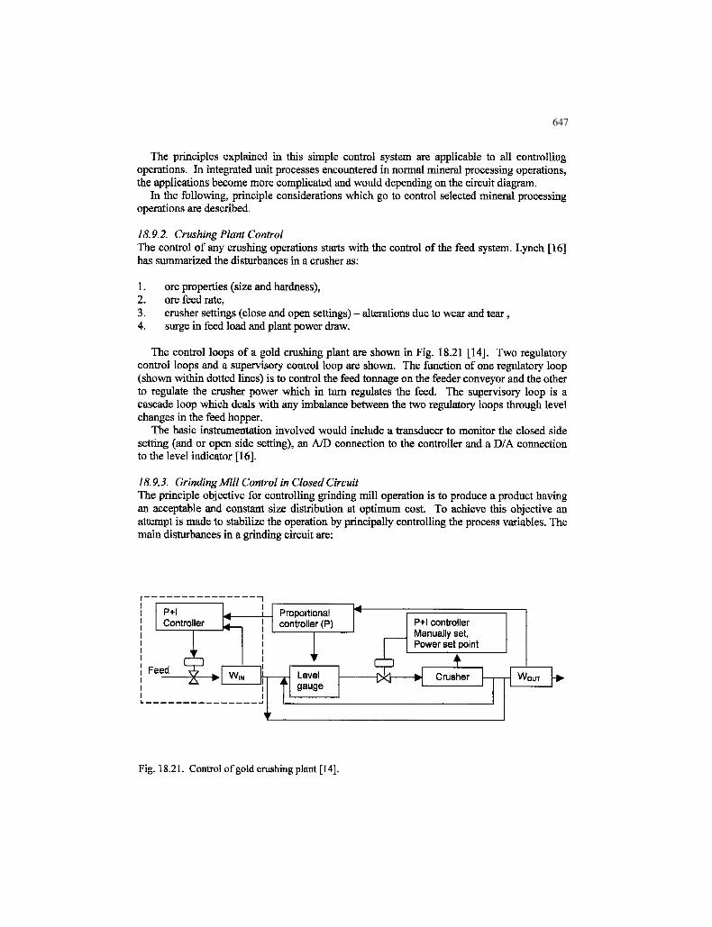
The control loops of a gold crushing plant are shown in Fig. 18.21 [14]. Two regulatorycontrol loops and a supervisory control loop are shown. The function of one regulatory loop(shown within dotted lines) is to control the feed tonnage on the feeder conveyor and the otherto regulate the crusher power which in turn regulates the feed. The supervisory loop is acascade loop which deals with any imbalance between the two regulatory loops through levelchanges in the feed hopper.
The basic instrumentation involved would include a transducer to monitor the closed sidesetting (and or open side setting), an A/D connection to the controller and a D/A connectionto the level indicator [16].
18.9.3. Grinding Mill Control in Closed CircuitThe principle objective for controlling grinding mill operation is to produce a product havingan acceptable and constant size distribution at optimum cost. To achieve this objective anattempt is made to stabilize the operation by principally controlling the process variables. Themain disturbances in a grinding circuit are;
P+lController
Feed
Proportionalcontroller (P)
Levelgauge
P+l controllerManually set,Power set point
fs.L/i Crusher Wo
Fig. 18.21. Control of gold crushing plant [14].
648648
1. change in ore characteristics (ore feed rate, grindability, feed particle size distribution,mineral composition and mineral characteristics like abrasiveness, hardness),
2. changes in mill operating parameters like variation of input flow rate of material likesurging of feed caused by pumps and level of mill discharge sump.
The mill control strategy has to compensate for these variations and minimize anydisturbances to the hydrocyclone that is usually in closed circuit. The simplest arrangement isto setup several control loops starting from the control of water/solid ratio in the feed slurry,sump level control, density control of pulp streams at various stages and control of circulatingload. Presently most mills use centrifugal pumps for discharging from the sump. This helpsto counter surges and other problems related to pumping. For feed control the most likelyoption is to use a feed forward control while for controlling the hopper level and mill speedand other loops the PI or PID controller is used. The control action should be fast enough toprevent the sump from overflowing or drying out. This can be attained by a cascade controlsystem. The set point of the controller is determined from the level control loop. This type ofcontrol promotes stability.
As an example, for completely controlling a grinding mill circuit the operation of a SAGmill is considered here as these mills seem to be slowly displacing the normal ball milloperations.
The SAG mill characteristics have already been mentioned earlier in Chapter 9. The mainvariables are:
1. solid mass transported through the mill ( solid feed plus the circulation load),2. the mill discharge solids, and3. the overflow solid flow.
From the control point of view, the additional interests are:
1. overfilling of the mill,2. grate restrictions and,3. power draft.
Each of these is controlled by specific controlled inputs, i.e., feed rate, feed water anddischarge water flows. The overflow solids fraction is controlled by monitoring the ratio oftotal water addition (WTOT) to the solid feed rate. The ratio being fixed by the target set pointof the overflow solid fraction.
Usually the charge volume of SAG mills occupy between 30-40% of its internal volume atwhich the grinding rate is maximized. When the charge volume is more, then the throughputsuffers. The fill level is monitored by mill weight measurement as most modern mills areinvariably mounted on load-cells.
During the operation of SAG mills, it is sometimes observed that the sump levels fallsharply and so does the power draft. This phenomenon is attributed to flow restrictionsagainst the grate. When this occurs it is necessary to control, (or in extreme circumstances),stop the incoming feed.
The power draft is the result of the torque produced by the mill charge density, lift angle ofthe charge within the mill and fill level. The relationship between these parameters iscomplex and difficult. Therefore to control mill operation by power draft alone is difficult.
649649
For the purpose of stabilization of the circuit, the basis is to counteract the disturbances.Also the set points must be held. The set points are attributed by dynamic mass balances ateach stage of the circuit.
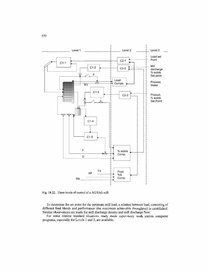
In modern practice the structure and instrumentation of the control systems of tubulargrinding mills are designed to operate in three levels or in some cases four levels. The controlloops and sensors for a SAG-mill and the levels of control are illustrated in Fig. 18.22.According to Elber [10,17], the levels are:
Level 1The operation at Level 1 mainly consists of controlling the feed rate and the water inputs. Inaddition to this the SAG mill revolving speed and secondary circulating load also formsancillary loops.There are four main control loops in Level 1 (Table 18.4).
Table 18.4Control loop of SAG mill
Control Loop Control VariablesFeed Flow rate Feeder Speed ( Feed motor speed)Sump water flow Valve positionSump level (Discharge feed regulator) Level indicator
The main sensors are:
1. load cell for mill weight,2. power measurement (ammeters, voltmeters), and3. density gauges (y-ray density gauge) for on line, non-invasive, measurement of slurry
densities.
Level 2The function of Level 2 is to stabilize the circuit and to provide the basis of optimizingfunction in Level 3. Three cascade loops operating in level 2 controls that function inconjunction with level 1 controllers. The cascade loops are:
The set points are supplied by level 3 controllers for all the cascade loops. The mill loadand percent solids in the two streams are calculated from signals received by sensors in thewater flow stream, the sump discharge flow rate and the density readings from density metersin the pulp streams. The mill load cells supply the charge mass. The load cell signals arecompensated for pinion up thrusts [10].
The set points for the mill load and the two pulp densities are given by level 3 controls.The points may also be set by neural method of analysis or fuzzy logic expert systems.
650650
Level 1 Level 2 h-
C1-1
C1-2
C2-1 t
C2-2
Wt
LoadCompo.
C1-3
XC2-3
C1-4
C1-5
% solidsComp.
Wf
Ws
Prod.%SComp.
Level 3
Load setPoint
Milldischarge% solidsSet point
ProcessWater
Product,% solidsSet Point
Fig. 18.22. Three levels of control of a AG/SAG mill.
To determine the set point for the optimum mill load, a relation between load, consisting ofdifferent feed blends and performance (the maximum achievable throughput) is established.Similar observations are made for mill discharge density and mill discharge flow.
For some routine standard situations ready made supervisory work station computerprograms, especially for Levels 1 and 2, are available.
651651
Level 3The primary function at Level 3 is optimisation of the SAG mill operation. That is, control ofthe product at optimum level. In an integrated situation where ball mill and cyclone is in thecircuit, the optimisation must take place keeping in mind the restraints imposed by downstream requirements. This optimisation can best be achieved by developing a software forcomputer use. Usually a large database is required to cover infrequent control actions.
18.9.4. Thickener ControlThe control of thickener operation is directed to obtaining a clear overflow as rapidly aspossible. The sedimentation rate is usually accelerated by additions of flocculants.Flocculants are added in the feed pipe (or feed launder) and maximum dispersion attemptedby appropriate design of its entry to the thickener tank. The object is to entirely cover all thesurface of mineral particles. The choice of flocculent and its concentration vary. It depends onthe minerals present in the slurry, their composition and their surface characteristics. It isnecessary not to have too much turbulence at the entry point of the tank.. For this purpose, theoverflow level is kept sufficiently high above the feed level to ensure acceptable solidconcentration in the overflow.
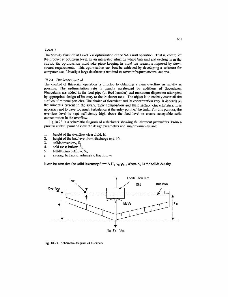
Fig. 18.23 is a schematic diagram of a thickener showing the different parameters. From aprocess control point of view the design parameters and major variables are:
1. height of the overflow clear fluid, H,2. height of the bed level from discharge end, HB,3. solids inventory, S,4. sold mass inflow, Si,5. solids mass outflow, So,6. average bed solid volumetric fraction, vs
It can be seen that the solid inventory S = A HB VS ps , where ps is the solids density.
hwFeed+Flocculent
) Bed levelOverflow
Fig. 18.23. Schematic diagram of thickener.
652652
At the bed level the solids residence time, tR will be:
tR = -I- (18.61)
The dynamic solids mass balance is:
dS( S S ) (18.62)
During operation, if the feed flow changes, i.e., increases or decreases, the flocculent inputchanges proportionately. A control loop in the flocculent charging device involving a pumpis required to follow these changes at an appropriate level of control.
The power, P, required by the pump, which is assumed to be connected to a horizontal pipewith no bends, is given by:
P = k n (FD)2 kW/h (18.63)
where k = constant (proportional to pipe length),[i = viscosity,FD = underflow discharge flow rate.
The pump pressure obviously varies as the solids mass outflow (kg/m3) and according toElber [10], is given by:
P = - r - ^ -S 2 0 .96 Pa (18.64)P Bs
2
Control StrategyThe control of the solid contents in the overflow and underflow streams is the basis ofthickener control. The average bed density (solids inventory) has to be controlled by theunderflow flow rate and the flocculent additions to the slurry. To attain target overflow solidsconcentration the underflow density should be sufficiently high. This is obtained by longerresidence time of treated slurry in thickener.
The underflow flow rate is measured by magnetic or ultrasonic flow meters.The control scheme can now be summarized:
Level 1: Control loopsTwo main loops are placed in Level 1. The first main loop (# 1) is for underflow control. Thesecond main loop (#2) is for the control of flocculent flow.At level #1, the essential process measurements for underflow control are:
1. rake torque with a torque meter fixed to the rakes,2. bed level by using a simple float or vertical position sensor,3. thickener bed pressure, by measuring the pulp pressure on the floor by a sensor.
653653
At level #2 for flocculent loop control, measurements are chiefly flow rates of fluids bystandard flow meters and power draft measurements for variable speed positive displacementpump. Other measurements at this level include:
1. pump speed,2. underflow density measurement (y-ray density gauge),3. pump discharge pressure by standard pressure gauge.
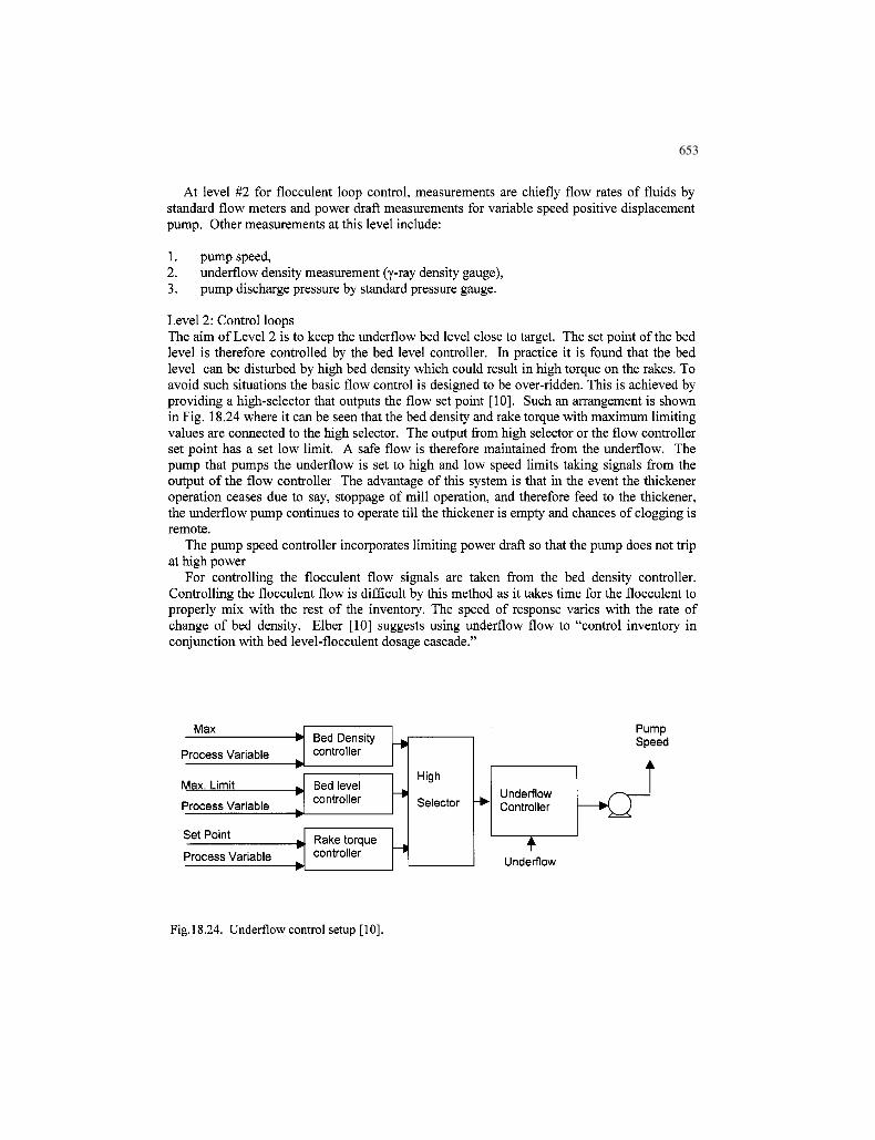
Level 2: Control loopsThe aim of Level 2 is to keep the underflow bed level close to target. The set point of the bedlevel is therefore controlled by the bed level controller. In practice it is found that the bedlevel can be disturbed by high bed density which could result in high torque on the rakes. Toavoid such situations the basic flow control is designed to be over-ridden. This is achieved byproviding a high-selector that outputs the flow set point [10]. Such an arrangement is shownin Fig. 18.24 where it can be seen that the bed density and rake torque with maximum limitingvalues are connected to the high selector. The output from high selector or the flow controllerset point has a set low limit. A safe flow is therefore maintained from the underflow. Thepump that pumps the underflow is set to high and low speed limits taking signals from theoutput of the flow controller The advantage of this system is that in the event the thickeneroperation ceases due to say, stoppage of mill operation, and therefore feed to the thickener,the underflow pump continues to operate till the thickener is empty and chances of clogging isremote.
The pump speed controller incorporates limiting power draft so that the pump does not tripat high power
For controlling the flocculent flow signals are taken from the bed density controller.Controlling the flocculent flow is difficult by this method as it takes time for the flocculent toproperly mix with the rest of the inventory. The speed of response varies with the rate ofchange of bed density. Elber [10] suggests using underflow flow to "control inventory inconjunction with bed level-flocculent dosage cascade."
Max
Process Variable
Max. Limit ^
Process Variable
Bed Densitycontroller
Bed levelcontroller
Set Point
Process VariableRake torquecontroller
High
Selector
PumpSpeed
UnderflowController
rUnderflow
Fig.18.24. Underflow control setup [10].
654654
Level 3: Control loopsLevel 3 control involves optimisation of thickener operation (and pipe lines). This includescost function based on:
1. flocculent consumption,2. pump power,3. discharges to tailings.
All these factors depend on the underflow density set point. Optimum conditions areusually ascertained by trial and error method by taking signals from the underflow density,pump discharge pressures and pump power drafts and estimating the corresponding costfunctions.
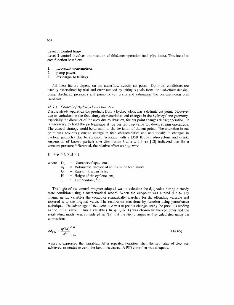
18.9.5. Control of Hydrocyclone OperationDuring steady operation the products from a hydrocyclone has a definite cut point. Howeverdue to variations in the feed slurry characteristics and changes in the hydrocyclone geometry,especially the diameter of the apex due to abrasion, the cut point changes during operation. Itis necessary to hold the performance at the desired dsoc value for down stream operations.The control strategy could be to monitor the deviation of the cut point. The alteration in cutpoint was obviously due to change in feed characteristics and additionally to changes incyclone geometry due to abrasion. Working with a D6B Krebs hydrocyclone and quartzsuspension of known particle size distribution Gupta and Eren [18] indicated that for aconstant pressure differential, the relative effect on dsoc was:
Du>(p, > Q > H > T
where Du = Diameter of apex, cm.,(pi = Volumetric fraction of solids in the feed slurry,Q = Rate of flow , m3 /min,H = Height of the cyclone, cm,T = Temperature, ° C.
The logic of the control program adopted was to calculate the dsoc value during a steadystate condition using a mathematical model. When the cut-point was altered due to anychange in the variables the computer sequentially searched for the offending variable andrestored it to the original value. The restoration was done by iteration using perturbancetechnique. The advantage of the technique was to predict changes using the previous readingas the initial value. Thus a variable (Du, <p, Q or T) was chosen by the computer and theestablished model was considered as / ( x ) and the step changes in dsoc calculated using theexpression:
Ad5oc -dx
(18.65)
where x expressed the variables. After repeated iteration when the set value of dsoc wasachieved, or tended to zero, the iterations ceased. A PID controller was adequate.
655655
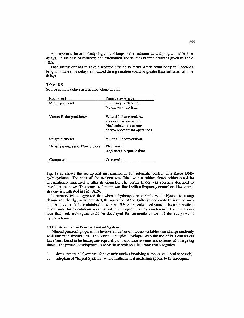
An important factor in designing control loops is the instrumental and programmable timedelays, hi the case of hydrocyclone automation, the sources of time delays is given in Table18.5.
Each instrument has to have a separate time delay factor which could be up to 3 secondsProgrammable time delays introduced during iteration could be greater than instrumental timedelays
Table 18.5Source of time delays in a hydrocyclone circuit.
Equipment Time delay sourceMotor pump set Frequency controller,
Inertia in motor load.
Vortex finder positioner Vfl and I/P conversions,Pressure transmission,Mechanical movements,Servo- Mechanism operations
Spigot diameter V/I and I/P conversions.
Density gauges and Flow meters Electronic,Adjustable response time
Computer Conversions
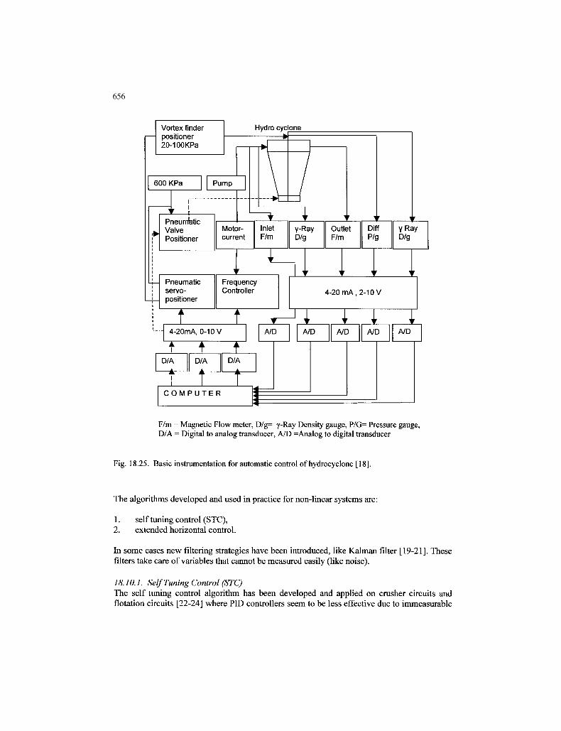
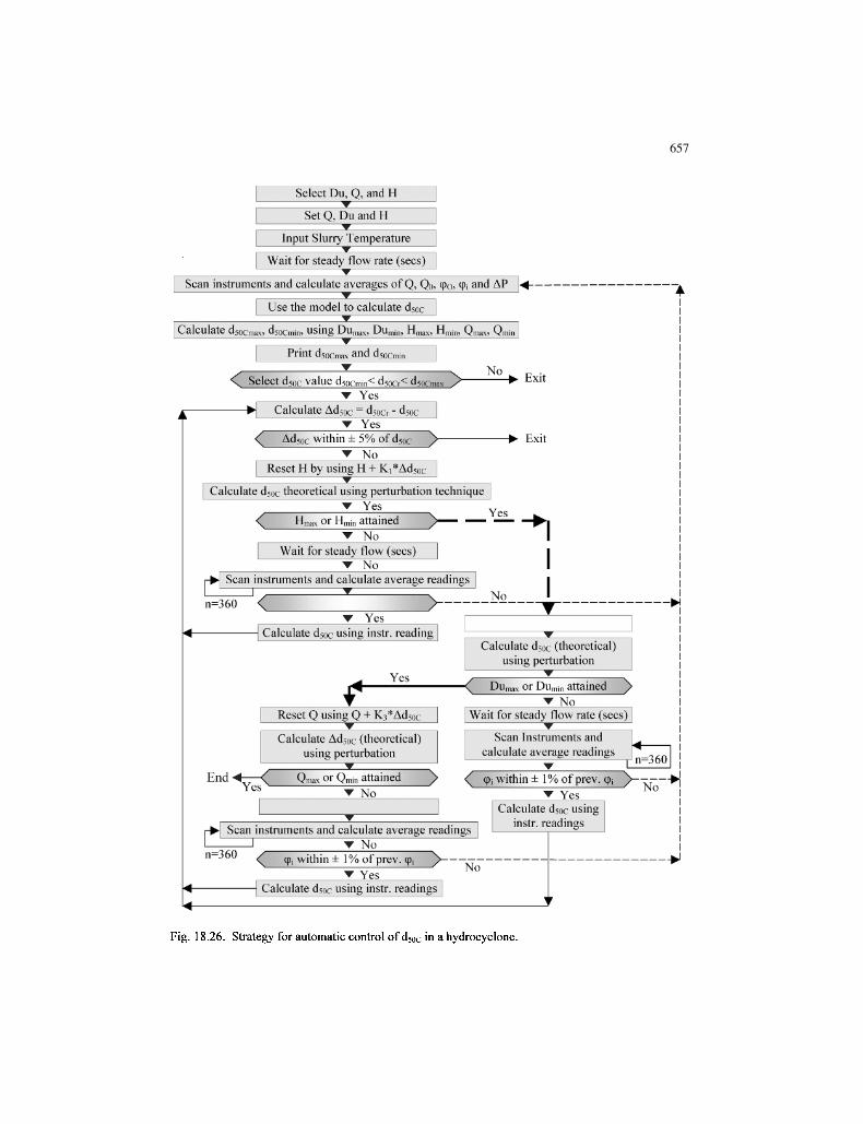
Fig. 18.25 shows the set up and instrumentation for automatic control of a Krebs D6B-hydrocyclones. The apex of the cyclone was fitted with a rubber sleeve which could bepneumatically squeezed to alter its diameter. The vortex finder was specially designed totravel up and down. The centrifugal pump was fitted with a fiequency controller. The controlstrategy is illustrated in Fig. 18.26.
Laboratory trials suggested that when a hydrocyclone variable was subjected to a stepchange and the dsoc value deviated, the operation of the hydrocyclone could be restored suchthat the dsoc could be maintained to within ± 5 % of the calculated value. The mathematicalmodel used for calculations was derived to suit specific slurry conditions. The conclusionwas that such techniques could be developed for automatic control of the cut point ofhydrocyclones.
18.10, Advances in Process Control SystemsMineral processing operations involve a number of process variables that change randomly
with uncertain frequencies. The control strategies developed with the use of PID controllershave been found to be inadequate especially in non-linear systems and systems with large lagtimes. The present development to solve these problems fall under two categories:
1. development of algorithms for dynamic models involving complex statistical approach,2. adoption of "Expert Systems" where mathematical modelling appear to be inadequate.
656656
Vortex finderpositioner20-100KPa
600 KPa
PneumaticValvePositioner
Hydro cyclone
Pump
Motor-current
InletF/m
y-RayD/g
OutletF/m
DiffP/g
yRayD/g
Pneumaticservo-positioner
FrequencyController 4-20 mA, 2-10 V
— 4-20mA, 0-10V
D/A
A/D
D/A D/A
C O M P U T E R
A/D A/D A/D A/D
F/m = Magnetic Flow meter, D/g= y-Ray Density gauge, P/G= Pressure gauge,D/A = Digital to analog transducer, A/D =Analog to digital transducer
Fig. 18.25. Basic instrumentation for automatic control of hydrocyclone [18].
The algorithms developed and used in practice for non-linear systems are:
1. self tuning control (STC),2. extended horizontal control.
In some cases new filtering strategies have been introduced, like Kalman filter [19-21]. Thesefilters take care of variables that cannot be measured easily (like noise).
18.10.1. Self Tuning Control (STC)The self tuning control algorithm has been developed and applied on crusher circuits andflotation circuits [22-24] where PID controllers seem to be less effective due to immeasurable
657657
Select Du, Q, and H
SetQ, Du and H
Input Slurry Temperature
Wait for steady flow rate (sees)
Scan instruments and calculate averages of Q, Qo, qjo, <p, and AP
Use the model to calculate d~
Calculate d^c™*, d5oc,,,i,,, using Du1118X, Du,nin, HrrsL,, H,,,,,,, Qrrlils, Q,lml
Print djocraas and dsoCmin
Select d5ij[.- va l ue d3ii^rT1iT1< d.^n;r< dSin.:max
• Yes•> Calculate Ad5rx: = djoci - dsoc
1"No
YesAdjuf within ± 5% of dVK:
• NoReset H by using H + K,*Ad5,
Exit
Exit
Calculate d o theoretical using perturbation techniqueYes
nas o r Il1Miii a t t a i n e dYes^ i cs
NoWait for steady flow (sees)
NoScat] instruments and calculate average readings
n=.16OYes
Calculate d?oc using instr. readingCalculate d uc (theoretical)
using perturbation
YesDu™ miii attained
Reset Q using Q + K3*Adan: Wait for steady flow rate (sees)
Calculate Ad50c {theoretical)using perturbation
Scan Instruments andcalculate average readings
EndYes
Qniax or Qmiii attained
n=36O
No<p; within ± 1% of prev. (pL
• YesT ,
Scan instruments and calculate average readingsI 1 • Non=360
Calculate d5oc usinginstr. readings
^ (Pi within ± 1% of prev. tpL y~-
• YesCalculate dw< using instr. readings
Fig. 18.26. Strategy for automatic control of d5Oc in a hydrocyclone.
658658
change in parameters like the hardness of the ore and wear in crusher linings. STC isapplicable to non-linear time varying systems. It however permits the inclusion of feedforward compensation when a disturbance can be measured at different times. The STCcontrol system is therefore attractive. The basis of the system is:
1. on-line identification of process model,2. use of the control model in the process design.
The mathematical basis of the process is the least square model. When the time delay, t, isgreater than zero, the process model is described in the predictive form [7].
The disadvantage of the set up is that it is not very stable and therefore in the controlmodel a balance has to be selected between stability and performance. A control law isadopted. It includes a cost function CF and penalty on control action. The control law hasbeen defined as:
where Osp = output set point,n = penalty on control action.
To obtain maximum stability and therefore minimum variance of the output, a suitableform of equation has been derived as:
Oc (t) = 2 ^ [{ a , OPR (t) + ..+ an OPR (t-n+1) + OSp } -
P [ pi Oc(t-1) + .. + p P 0 c ( t - P ) ] ~ (18.67)
where Oc(t = output Controller at time t,OSP = output ser point
OPR (t) = output (Process) at time t,s(t) = error at time t,t = time,n = order of system,k = constant,a, P = parametersJC = n + t - 1
The parameters a and P are estimated by setting up a suitable algorithm and calculated fordifferent times. When n = 0, then n + t = 1 . Eq. (18.67) acts as a self tuning regulator [6].
In some cases, like the control of a crusher operation, a constant term has to be introducedin Eq. (18.67) as at zero control action and the crusher operates at steady state.
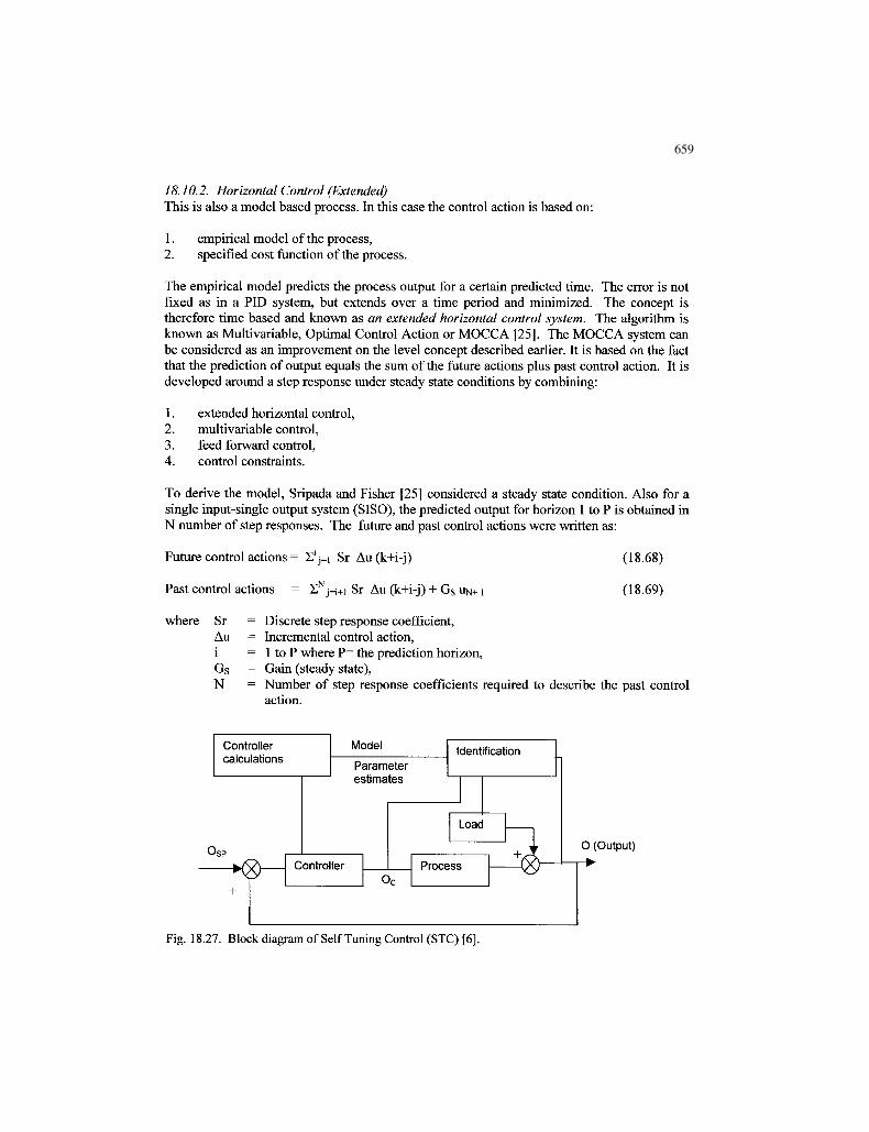
A block diagram showing the self tuning set-up is illustrated in Fig. 18.27. Thedisadvantage of STC controllers is that they are less stable and therefore in its application abalance has to be derived between stability and performance.
659659
18.10.2. Horizontal Control (Extended)This is also a model based process. In this case the control action is based on:
1. empirical model of the process,2. specified cost function of the process.
The empirical model predicts the process output for a certain predicted time. The error is notfixed as in a PID system, but extends over a time period and minimized. The concept istherefore time based and known as an extended horizontal control system. The algorithm isknown as Multivariable, Optimal Control Action or MOCCA [25]. The MOCCA system canbe considered as an improvement on the level concept described earlier. It is based on the factthat the prediction of output equals the sum of the future actions plus past control action. It isdeveloped around a step response under steady state conditions by combining:
To derive the model, Sripada and Fisher [25] considered a steady state condition. Also for asingle input-single output system (SISO), the predicted output for horizon 1 to P is obtained inN number of step responses. The future and past control actions were written as:
Future control actions = S'j=i Sr Au (k+i-j)
Past control actions = E j=i+i Sr Au (k+i-j) + Gs UN+ I
(18.68)
(18.69)
where Sr = Discrete step response coefficient,Au = Incremental control action,i = 1 to P where P= the prediction horizon,Gs = Gain (steady state),N = Number of step response coefficients required to describe the past control
action.
O (Output)
Fig. 18.27. Block diagram of Self Tuning Control (STC) [6].
660660
The predicted output, O (k+1) is the sum of Eqs. (18.68) and (18.69), that is:
O (k+i) = X1 j=i Sr, Au (k+i-j) + SN
J=.+i Sr, Au (k+i-j) + G uN+ 1 (18.70)
We can see that Eq. (18.70) is applicable for prediction of horizon P where i = 1 to P andfor control horizon H where i - j >H.
The predicted horizon P, is the number of predicted outputs that the control objective hasbeen optimized The control horizon H is the number of future control actions which minimizethe cost function against the predicted horizon.
Optimization of the control system is achieved from performance criteria including anyconstraints. It is necessary to know the set point and predicted output trajectories for futurecontrol effort. The errors and control efforts have to be minimized. For the error trajectory thesquare of the difference of set point trajectory and the predicted output trajectory is taken.Taking these into consideration Vien et al [6] describes the cost function, Cf, in terms ofminimizing the error trajectory plus control effort. Taking the weighted least squareperformance, the cost function Cf is given as:
where Spr = set point trajectory,OPT = predicted output trajectory,A UF = future control effort, andTM = input weighting matrices,Tw = output weighting.
The first term in Eq. (18.71) is for minimizing error trajectory and the second term is forminimizing control effort.
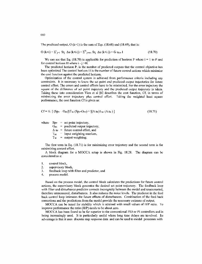
A block diagram for a MOCCA setup is shown in Fig. 18.28. The diagram can beconsidered as a:
1. control block,2. supervisory block,3. feedback loop with filter and predictor, and4. process model.
Based on the process model, the control block calculates the predictions for future controlactions, the supervisory block generates the desired set point trajectory. The feedback loopwith filter and disturbance predictor corrects incongruity between the model and unaccounted,therefore unmeasured, disturbances. It also reduces the noise levels. The predictor in the feedback control loop intimates the future effects of disturbances. Combination of the feed backcorrections and the predictions from the model provide the necessary estimate of output.
MOCCA can be tuned for stability which is attained with small values of H/P ratio. Toimprove performance the ratio (H/P) needs to be about zero.
MOCCA has been found to be far superior to the conventional PID or PI controllers and isbeing increasingly used. It is particularly useful where long time delays are involved. Itsadvantage is that it uses discrete step response data and can be used to model processes with
661661
Load
Supervisorysystem
ControlAlgorithm
Process.0 (Output)
Processmodel
Predictor Filter
Fig. 18.28. Block diagram of MOCCA control system [6].
unusual dynamic behaviour. Its added advantage over the PID system of control is that itrises faster and has no overshoot. This system has been used successfully in control ofgrinding circuits.
18.11. Expert Systems
18.11.1. Fuzzy System of ControlSo far we have assumed that the numerical solutions are possible in the control of processoperations. There are however many instances when numerical methods cannot be applied,such as the gradual effect of wear and tear on the mill liners, spigot diameter change in ahydrocyclone operation or the effect of such energy consuming phenomenon like noise.Difficulties are compounded by the large number of variables in an operation and non-linearrelationships. In such cases, heuristic search for answers have been sought. Naturallyheuristic approach results in, some answers that are correct, others are not. Or some answersmay be satisfactory and acceptable while others are not. In mineral processing operations,operators generally use their common sense to arrive at an answer some of which aresatisfactory and produce required grades and recoveries. That is, with their acquiredknowledge and skills they are able to control systems satisfactorily. Knowledge is anintellectual property gained by experience, but it can be quantified, say from 0-1 where, 0 isthe least and 1 represent maximum knowledge. The numbers in between may be referred toas different degrees otherwise shades of knowledge. Linguistic forms of knowledge thusexpressed in numeric form has been characterized and known as Fuzzy thinking according tofuzzy rules [27,28].
The symbolic language developed by experience can be put in expert system shells in theusual programming languages. The knowledge may be stored in frames or production rulesor in the form of combined frame and production rules. The frame is a technique which foran object allows the specification of object and allotment of slots associated with that object.
662662
Thus in the mineral industry, a flotation cell or a tumbling mill will be the object and the slotsare attributes. In a flotation system the attributes are items like froth depth, cell capacity, airand so on. Zadeh [26] considered the above concepts and applied it to control strategy.According to this theory, an element x is either a member of a set HA(X), or not a member of aset. That is, it is based on a binary system which can be expressed as:
1 if x is a member of A,Membership of set A, UA(X) =
0 if x is not a member of A
Thus a fuzzy set A is characterized by a membership function represented as uA(x) where xis the membership number of x in A and x an assigned number (say) between 0 and 1. Thefuzzy sets can be combined to form fuzzy subsets. Thus the union of sets A and B may bewritten as AuB. They can also intersect (AnB). The basic operations may be written as [36]:
where x and y are the two variables defined for sets A and B. Set A may be considered as theinput variable while set B is the output variable.
From the process control aspect the relation between A and B may be written using fuzzyrelationship in the form of IF and THEN. That is:
IF error is large THEN control action is large
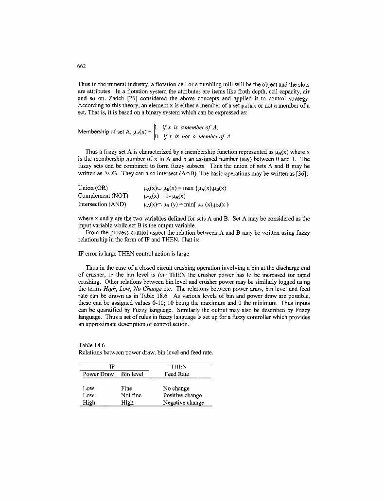
Thus in the case of a closed circuit crushing operation involving a bin at the discharge endof crusher, IF the bin level is low THEN the crusher power has to be increased for rapidcrushing. Other relations between bin level and crusher power may be similarly logged usingthe terms High, Low, No Change etc. The relations between power draw, bin level and feedrate can be drawn as in Table 18.6. As various levels of bin and power draw are possible,these can be assigned values 0-10; 10 being the maximum and 0 the minimum Thus inputscan be quantified by Fuzzy language. Similarly the output may also be described by Fuzzylanguage. Thus a set of rules in fuzzy language is set up for a fuzzy controller which providesan approximate description of control action.
Table 18.6Relations between power draw, bin level and feed rate.
IFPower Draw
LowLowHigh
Bin level
FineNot fineHigh
THENFeed Rate
No changePositive changeNegative change
663663
Table 18.6 shows that the basic operations are simple though there is an element ofvagueness. The vagueness can be quantified and a fuzzy algorithm developed to convertfuzzy input to fuzzy output using available software. The association of rules governing thefuzzy controller is the fuzzy decision algorithm for process control. Harris and Meech [29]lists the following actions to develop fuzzy rules:
1. observe and interview operator,2. identify and standardize the linguistic process variables,(high low, bad not-bad etc)3. define membership functions of fuzzy sets that represent linguistic variable, and4. assemble fuzzy rule strategy.
The output of a fuzzy system is also fuzzy expressed in membership values of eachvariable in a process. It is therefore necessary to defuzzify using an inference process to adiscrete value. The inferencing process can be a data driven search to obtain a goal orconclusion. This is known as forward chaining. It can also be a goal driven search where thegoal is assumed and available data examined to support or reject it. This is known asbackward chaining. The inferencing process is generally known as an Inference Engine. Afuzzy logic control system of a process is illustrated in Fig. 18.29.
The implementation of fuzzy logic control is presently done by using software that arecommercially available. In complicated process control systems, like the control of flotation,fuzzy logic has been integrated with conventional PID systems.
A survey of literature indicates that Fuzzy system of control has been used mostly inmilling and flotation circuits [30-34]. Freeman et al [32] has indicated an increase inproductivity in the gold milling circuit at Kalgoorlie Consolidated Gold Mines, Fimiston Plantand increased stability in alumina grinding at the Comalco Bell Bay plant.
The greatest advantage of the use of Fuzzy logic is that it can tackle non-linear systemsand such systems that are difficult to use mathematically. It may be mentioned that eventhough the Fuzzy control system may appear simple and has obvious advantages as it takesinto account non-measurable variables in a process, in practice considerable effort is requiredto control the tuner.
Load/disturbance
De-fuzzi
De-fuzzified
fication
controlsr
Process
Fuzzy Algorithm
Output
Non-Fuzzydimensions
r
Fuzzification
Fig. 18.29. Fuzzy Control System.
664664
18.11,2, Neural and Artificial Network Methods (ANN) of ControlThe alternate methods of control where conventional methods are unsatisfactory andprocesses that are non-linear are;
We shall only deal with the ANN method. This method helps to stabilize and control aprocess. Its set up is easier and it does not require elaborate statistical work orphenomological data collection. Eren and Fung [36] describe the method as "a mapping frommeasurement history to commands". Mapping involves machine learning which is usuallyreferred to as artificial intelligence. The ANN is a branch of artificial intelligence and isbeing increasingly applied to complex mineral processing operations like flotation [37].
A neural network consists of a box containing single computational elements known asneurons. The neurons exist in layers and are dynamically interconnected by synapses. Thearrangement of interconnections of the neurons or topology is fixed by the designer. Eachneuron has an internal parameter called weight. Each neuron is a processing element or nodeand forms an input-output field. The information contained in the nodes is the weight andlink-field. Each neuron output is a single numerical activity. The function of the elements(node) is to add the weighted inputs and pass the results to the next layer using a non-linearsigmoidal function of the type:
where cy = activation of neuron j ,P = steepness of activation function,cp = applied input potential.
The input potential, q>, to each neuron is defined in terms of the synapses and weightsbetween the neurons i and j and the threshold of neuron j , thus:
q> = 2 Sjj qj + Tj (18.73)
where Sy = Synapses weight between neurons i and j ,tj = Threshold of neuron j
Neurons get activated when the value of the sigmoidal function is greater than thethreshold value (T.J ).
A simplified three layer arrangement of neurons is illustrated in Fig. 18.30 where it can beseen that each neuron in the first layer receives weighted inputs I], I2,13 and I4. Output fromeach neuron in a layer is then passed on to each neuron in the following (right) layer and theoutputs from each neuron in the second layer activate neurons in the subsequent layer, thisultimately results in an output. Each neuron undergoes a non-linear transfer function which issigmoidal in character.
According to Cortez and Durau [36] three layers of neurons are generally sufficient tosolve non-linear situations. The number of hidden neurons in a net-work is estimated from thenumber of input and output neurons. Thus if a vector of n number of neurons is in a input
layer and m neurons in the output layer, then the intermediate hidden middle layer would have2m + 1 neurons.
Neurons are trained by the input of values required by the operating system. When thevalues produce a sigmoidal function greater than the preset (or threshold value), then theelement is activated and sets to the trained value.
Two variations of ANN arrangements are used to control processes. They are the Backpropagation method and the Feed forward back-propagation (EBP) method. Of these, EBP isthe preferred method. Fig. 18.31 illustrates the EBP setup.
Training technique of EBP involves estimation of error which is the difference in outputpattern (produced by forward pass) and the target value. Starting from the output, the error isworked back progressively to the input layer of neurons. In so doing, a gradient of error isestablished between neurons. The gradient is summated for each weights associated witheach neuron for all input - outputs. Due to establishment of the gradient, the weights W; jhave to be revised and updated. For neurons i and j the updated weight would be:
Se(18.74)
where LR = learning rate,N = Nth. Iteration,E = summated error.
The learning rate LR is a discrete step size. Care must be taken regarding the step size, as ahigh value of LR will give a large value of W which will make the system unstable, again if alow value of LR is adopted then convergence will take a long time.
Updating is achieved by iteration till error for outputs are reduced to acceptable limits.Application of Eq. (18.74) is tricky due to difficulty of choosing the appropriate step size. Toease the problem a momentum term [M(AWjj)""1 is added to Eq. (18.74) where M is themomentum term and has a value 0 to 1.
666666
o.
In
Input Hidden Outputlayer layers layer
Fig. 18.31. EBP Artificial neural network [37].
Once trained, the ANN can accept linear and non-linear discrete or continuous functions. Theoperator can then take the help of established mathematical software, like MATLAB orsimilar package to control the system. The software must be supported by appropriatehardware.
18.12. Mechanics of Digital Process Control SystemsThe modern process plants are increasingly controlled by computers and digital devices.
But the signals generated by the processes are in analogue, therefore the analogue informationacquired are converted to digital form. The analogue to digital (A/D) converter is used forsignal conversion (Fig. 18.26). Usually multiplexers and sample-and-hold together devicesare included. The multiplexer enables connection to several transducers to same sensors andtransducers to the same signal processing media if required.
Digital systems are particularly useful in performing mathematical operations, numericdisplays when required, also for storing and transmitting information. It is particularly usefulfor the application of specific software.
Microprocessors and microcontrollers constitute the heart of almost all types of digitalprocess control systems. They play an important role in data handling data processing andcontrol. Application of micro-processors are in the field of data handling which includes dataacquisition, data processing, interpretation, storage and communication. It is also used forinstrumentation control of sensors and actuators. Microprocessors provide a meaningfulhuman-machine interface. Micro-controllers and digital signal processors are special micro-processors, the difference is in the degree of specialization.
IS. 12,1. Inputs and OutputsThe inputs and outputs of a process controlling system is usually performed through a dataacquisition hoard with 8-16 number of analogue inputs. These boards are the key elements to
667667
connect a computer to a process in order to measure or control its operation. The dataacquisition board is made up of an analog multiplexer, an amplifier (with programmable gain)a sample and hold circuit and A/D set up. The data acquisition board also offer analogueoutputs to carry control operation and also supply I/O lines and counters. The counters areused for applications such as counting the number of times an event offers (see Fig. 18.26)
18.12.2. Process Communications and NetworkIn process control instruments are often networked by computers to measure variables of aprocess. The arrangement for performing the overall measurement is called a measuringsystem.
In measuring, the information generated by each device is communicated between theinstruments themselves or between other devices like recorders and display units.Transmission of data are done easily by digital control systems, however as the measurementsystem becomes large as a result of inclusion of many instruments, the communication tocomputers can become complex. In such cases, the devices are networked either in groups oras a whole by a central computer. The standard networking topologies like star, ring field busare used.
Digital network is applied to Direct Digital Control (DDC) and Supervisory control. Ofmore interest to mineral processing systems are:
1. programmable Logic Controllers (PLC), and2. supervisory Control Data Acquisition (SCADA).
The Programmable logic controllers are industrial computers in which the hardware andsoftware has been specially adapted to a particular environment. They are therefore dedicatedcomputers.
The PLC works by continually scanning a program, for example, see Fig.18.26, where thereiteration and data have been scanned 360 times, the average taken and computationprogressed as per mathematical model established for the process. The scanning cycleconsists of 3 main steps as seen in Fig. 18.32.
f
Input Status
r
Execute Program
r
Update Output Status
r
Fig. 18.32. PLC Operation Cycle.
668668
The input modules take AC or DC 240V and converts to logic level 0-5V signals. Theoutput AC modules are Triac driven and are arranged in sink configuration. The DC outputmodules are controlled by transistor circuits.
The Supervisory Control Data Acquisition (SCADA) is used to monitor and controldistributed systems from a master location. It serves as an umbrella for the control ofproduction (including tailings), stockpiling and shipments. It finds application for controlling,scanning, monitoring data and data acquisition. It has three main components:
1 multiple remote terminal units,2 central control room with host computers, and3 software support.
While the remote terminal units are used to acquire data from physical devices like sensors,pumps, actuators, the central control units acting as host computers allows for supervisorylevel control of remote sites. It also provides the human-process interface that is, it permitsoperators to view and if necessary control any part of the plant equipment. SCADA softwaresare written in terms of pre-defined variables suitable for a particular operation.
18.13. Problems
18.1A decaying metallurgical process is expressed by the differential equation:
dtThe initial condition is x(0) =0 Trace the decay curve for 5 seconds.
18.2The response function of a process is given by:
dx— + x = 5dt
The initial condition is x(0) = 0. Draw the curve for t = 1-5 seconds.
18.3A process is defined by the equation:
d2x . dx—r- + 4x — + 4x =1dt2 dt
The base conditions are: x(0) =x'(0) =0Determine the nature of the curve and the limiting value.
18.4The output and input transfer functions ratio of a process is given by:Y(S) _h+\
X(S) T2+2
669669
If in an unit step function x(t) is applied, determine:
1. Y(t)
2. Draw the curve Y(t) against — when — = 3T2 T2
18.5A lime mixing tank having cross-section lm2 is operated at a steady level of 0.6 m. The limesuspension is removed for a gold treating plant at a constant rate of 0.3 m3 per min.irrespective of head. The resistance at the outlet valve R equals 1.7 m/m3. If the input rate isQ m/m and h(t) the height of the liquid level, determine the transfer function h(s)/Q(s).
18.6A proportional controller is used to control the level of a sludge tank between 3.0 and 3.1 m.The controller is operated pneumatically such that it goes from 1-5 when in fully open andfully shut positions and the level from 3.05 to 3.75 m with the set point held constant.Determine:
1. the proportional band,2. gain,3. if the proportional band was doubled what will be the level change.
18.7The level of a CIP tank was controlled by a controller as in Fig. 18.30 that was operatedpneumatically. It was found that the control output pressure changed by 2000 N/m2 for 1.0 mvariation in level. If the pressure changed by 4000 N/m2 resulted in a change from fully opento fully closed position of the controller valve. Determine:
1. the gain,2. the proportional band.
18.8An open loop system performs in the same manner as its transfer function. A unit step wasapplied as shown in the diagram and from the trace of response recorded below, determine thesettings of a PID controller.
<)— Controller -•//—!
IL
_^. final controller
- • Chart
1 Sensor
PrnnpsR
670670
Time, Response Time, Response Time, Responsesees sees sees
REFERENCES[I] J.G. Ziegler and N.B. Nichols, ASM, 64 (1942) 759.[2] G.H. Cohen and G.A. Coon,, Theoretical considerations of activated control
Trans ASME, 75 (1953) 827.[3] J.M. Coulson and J.F. Richardson, Chemical Engineering, Vol.3, 2nd (ed)., Pergamon
Press.[4] A.M. Lopez, C.L. Smith and P.W. Murill, British Chem. Eng., 14 (1969) 1533.[5] D.L. Rivera, M. Morari and S. Skogestad, Industrial Eng. Progress Design Dev., 25
(1986) 252.[6] A. Vien, R.P. Edwards and B.C. Flintoff, International Conference on Process Control,
Jan. 1998, pp. 337-352.[7] A. Vien, B.C. Flintoff and R.P. Edwards, 24* Canadian Mineral Processors
Conference, Ottawa, 1992, paper 6, pp. 1-8.[8] B.C. Flintoff, Control of Mineral Processing Systems, Preprint.[9] G.A. Gault, Process Control Lecture Series, WA. School of Mines, Kalgoorlie, Private
Communication. 1984.[10] L. Elber, Process Control for Mineral Processing and Metallurgists and Engineers,
Lecture Series, WA School of Mines, Private Communication, 1990.II1] G. Stephanopoulos, Chemical Process Control, Prentice Hall International, 1984.[12] B. Flintoff and A. Mular, A practical guide to process controls in Mineral Industry,
Gastown printers, 1992.[13] L. Anderson, R. Perry, A. Neale, International Conference on Process Control, Paper
No. 24,1998, pp. 359-379.[14] J.W. Austin, Vancouver CMP presentation, Dec 4., Pre-print, 1987.[15] N.P. Cheremisinoff, Process Level instrumentation and Control, Marcel Dekker, New
York and Basel, 1981.[16] A. Lynch, Mineral Crushing and Grinding Circuits, Elsevier Amsterdam, 1977.[17] L. Elber, Proceedings SAG/SEM 1989 Aus.I.M.M., Australia Nov., 1989.[18] A. Gupta and H. Eren, Proceedings, Aus.I.M.M., 295 No. 2 (1990) 31.[19] P.M.Bamham and D.E. Humphreys, Theory and Applications of Kalman Filtering, C.
Leondes (ed), AGARD Monograph, 139 (1970) 45.[20] B.W.Leach, Report NRC-NAE-MWC-57, National Research Council, 1984.[21] O.A. Bascur and J.A. Herbst, in Design and Installation of Concentration Circuits, A.L.
Mular and M.A. Anderson (eds), 1986, p. 835.
671671
[22] U. Borrison, and R. Syding, Automatical 2 (1976).[23] E.V. Manlapig, A.J. Thorton and G. Gongalez, Copper 87, Vol 3, A.Mular, G.
Gonzalez and C. Barahona (eds), CIM Chile, 1987, p. 387.[24] M. Frankin, in Process Control and Automation in Extractive Metallurgy, E.Partelpoeg
and D. Hammestoete (eds), AUME, 1989.[25] N.R. Sripada and D.G. Fisher, Multivariable, Optima, Constrained Control Algorithm
(MOCC A) Part 1, Formulation and application, Department of Chemical Engineering,University of Alberta, 1984.
[26] L.A. Zadeh, Fuzzy Sets Information and Control, Vol.3, 1965, pp. 338-353.[27] L.A. Zadeh, IEEE Transon System Mon. and Cyb., SMC-3, No. 1, 1973, pp. 28-34.[28] L.A. Zadeh, IEEE, Spectrum, Aug, 1984, pp. 26-32.[29] C.A. Harris and J.A. Meech, Fuzzy Logic: A potential control technique for mineral
processing, 24th Annual Met Conference, Vancouver, 1985.[30] L.C. Hales, Proceedings of the Engineering Foundation Conference, Dec. 1989, pp.
289-302.[31] C.A. Harris and G.A. Kosick, 20th Annual Meeting of Canadian Mineral Processors,
Ottawa Ontario, 1988, p. 149.[32] N. Freeman, W. Keenan, S. Hancock and G. Lepage, 5th Mill Operators Conference,,
Aus. I.M.M., Roxby Downs, 1994, pp. 193- 199.[33] M.J. Burrows, J.D. Carriere, J. Leung and D. Laguitton, 21st. Annual Meeting of
Canadian Processors, Ottawa, 1989.[34] J.A. Herbst, W.T. Pate and A.E. Oblad, Advances in Autogenous and Semi-
Autogenous Grinding Technology, A.L. Mular and G.E. Agar (eds), University ofBritish Columbia, 1989, p. 669.
[35] L. Cortez and F. Durao, APCOM XXV 1995 Conference, Brisbane 9-14 July, 1995,pp. 39-43.
[36] H. Eren and C.C. Fung, Automation and Control Equipment, private communication.[37] H. Eren, C.C. Fung and A. Gupta, Aus.IMM Annual Conference, Perth, 1996, pp. 225-
229.
Symbols and Units
A general convention used in this text is to use a subscript to describe the state of the quantity, e.g. Sfor solid, L for liquid, A for air, SL or P for slurry or pulp, M for mass and V for volume. A subscriptin brackets generally refers to the stream, e.g. (O) for overflow, (U) for underflow, (F) for feed, (C) forconcentrate and (T) for tailing. There are a number of additions to this convention which are listedbelow.
a a constanta amplitude map particle acceleration m/s2
A a constantA aperture micronsA area m2
Ac cross-sectional area m2
Ai abrasion indexAy assay of particles in the ith. size and j t h . density fractionsAE effective area m2
AEFF areal efficiency factorAo open area %A0E effective open area %A M assay of mineral %, g/t, ppmAy underflow area m2
b a constantb Rosin-Rammler distribution parameterBy breakage distribution functionc a constantC a constantC circulation ratio or loadC concentration, (mass solid/volume of slurry) kg/m3
CA concentration of air kg/m3
Cc average concentration of solids in the compression zone kg/m3
CD drag coefficientCi concentration of species i kg/m3
Co initial concentration (mass of solid/volume of slurry) kg/m3
CMAX maximum concentration (mass of solid/volume of slurry) kg/m3
C t concentration at time t (mass of solid/volume of slurry) kg/m3
CS(c) concentration of solid (C = concentrate, F = feed, T = tailf = froth, P = pulp)
Cu, CF concentrations of the underflow and feed respectively, kg/m3
(mass of solid/volume of slurry)CCRIT critical concentration kg/m3
CF correction factorCI confidence intervalCR confidence rangeCS(u) solids concentration in the underflow (O = overflow,F = feed) %
concentration by mass of solids in the feed %
xvi
CvS(F)
cccvCoo
ddd32
dN
dso, dsocdB
dF
dL
dMAX
dMIN
d\iiD
dcutter
dcdwDDD*DcD,DoDueEiEc
EEcEB
EoEoEPEuET
/
/ (JB)
As)/P,/F
fiFmicronsFFFFi
concentration by volume of solids in the feedconcentration criterioncoefficient of variationconcentration at infinite timea constantparticle size, diameterSauter mean diameternominal diametercut or separation size, corrected cut sizeball diameter63.2% passing size in the feedliberation sizelargest dimensionsmallest dimensionmid-range dimensioncutter openingcylpeb diameterwire diameterdischarge mass ratio (liquid/solid)displacement, distance, diameterdimensionless parametercyclone diameterinlet diameteroverflow diameterunderflow diametera constantpartition coefficient of size i = recovery of size i in the U/Fcorrected partition coefficientenergycorrected partition coefficientenergy of reboundspecific grinding energyefficiency based on oversizeEcart probability, probable error of separationefficiency based on undersizetotal energya constantball wear rateball load-power functionsuspensoid factorfunction relating to the order of kinetics for pulp and frothmass fraction of size i in the circuit feedfeed size
floats at SGfroth stability factorfeed mass ratio (liquid/solid)settling factor
80% passing size of feedRowland ball size factorbuoyancy forceBond mill factorcentrifugal forcedrag forcegravitational forcecorrection factor for extra fineness of grindcorrection factor for oversized feedcorrection factor for low reduction ratiomass flow rateBond slurry or slump factorgravitational constant (9.81)grade (assay)net grams of undersize per revolutiongrinding parameter of circulating loadfree energyparameter = X/CTdiatances within the conical section of a millhindrance factorheightheight at time theight of rebound pendulumheight of bedheight of ball chargeheight of the start of the critical zone in sedimentationheight of the clarification zone (overflow)height of resthindered settling factormudline height at the underflow concentrationheight after infinite timeimpact crushing strengthimperfectionfraction of mill volume occupied by bulk ball chargefraction of mill volume in cylindrical section occupied by ballsand coarse oresuperficial gas velocityfraction of mill volume occupied by bulk rock chargefraction of mill volume filled by the pulp/slurryconstantrate constant for air removal via froth and tailings respectivelyrate constant for fast and slow component respectivelycomminution coefficient of fraction coarser that ith screenscreening rate constant, crowded condition, normal and half sizescreening rate constant, separated condition, normal and half sizeconstantmaterial constantkinetic energy
microns-N-NNN---kg/s,t/h-m/s2
%, g/t, ppmg/rev-J-m-m, cmmmmmmmm-mmkg.m/mm---
m/s----min"1
-t/h/m2
m1
--kW
xviii
LLA
LAE
LEFF
LcLcYL, LcONELF
L M W , LMAX
LTI_I
LVF
mmmuoomk
mu(O)m(r)mT
mu(o>mi(U)
MMiMoi
MyMB
M B
Mc
MeMF
M F
M F T
M F
MMIN
MR
M R
MrMs
Ms
lengthaperture sizeeffective apertureeffective grinding lengthlength of cyclonelength of cylindrical and cone sectionsNordberg loading factorminimum and maximum crusher setcrusher throwlength of vortex finderlength from end of vortex finder to apex of a cyclonemoisture (wet mass/dry mass)mineralogical factormass fraction of undersize in the feedmass fraction of makeup balls of size kmass fraction of undersize in the oversizecumulative mass fraction of balls less than size rmass rate of ball replacement per unit mass of ballsmass fraction of undersize in the undersizemass of size i in the underflow (F = feed)massmassmass/mass fraction of i* incrementcumulative mass fraction retained on i* screen at zero timemass percent of the i* size fraction and j * density fractionmass of blockmass of ballsmill capacitymass of crushing weightmass of feedmass of fluidmass of floatsNordberg mill factorminimum mass of sample requiredmass of rockmass fraction of rock to total charge (rock + water)cumulative mass fraction of balls of size r in the chargemass of striking pendulummass of solid
mmmmmm-mmmm-kg/m3
---kg/h.t-kggkg,tkg,t
%kgkgt/hkgtkgkg,t-kg,tkg
-kgke,t
. sec), SOD n ^ 5 of solid feed, concentrate and tailing respectively kg, tmass of solid in froth
MSK mass of sinks kg, tMS{p) mass of solid in the pulp kg, tAM(t) mass of top size particle kg, tMj mass of new feed gMw mass of water kg, tn number of revolutions/min min"1
n number of increments, measurements
xix
nn(r)nsNNNNL
N'Oi
PPiPPsoppppppPA, PC, PE, PF
PcON
PCYL
PD
PG
P«PL
PM
PM
PNET
PNL
PosPR
PsPsPEAPqQQB
QH
QoQuQMSOT
QMSCQ
QM(F)
Qv(C), (T), (F)
QvL(O)
order of rate equationcumulative number fraction of balls of size less than rnumber of sub-lotsnumber of mill revolutionsnumber of strokes/minnumbernumber of presentations per unit lengthnumber of particles/grammass fraction of size i in the overflowbinomial probability of being selected in a samplemass fraction of size i in the new feedproduct size80% passing size of productproportion of particlespressurePowers roundness factorJig powerJKSimFloat ore fioatability parameterprobabilityprobability of adherence, collision, emergence, froth recoverypower of the conical part of a millpower for the cylindrical part of a millparticle distribution factorproportion of gangue particlesproportion of particles in the i . size and j * . density fractionsliberation factorproportion of mineral particlesmill powernet mill power drawno load powerperiod of oscillationrelative mill powerparticle shape factorpower at the mill shaftpotential energypressure dropalternate binomial probability = 1 — pcapacitymakeup ball addition ratebasic feed rate (capacity)tonnage of oversize materialcapacity of the underflowflowrate of solids by mass in the overflow (U = U/F, F = feed)mass flow of solid in concentratecapacity, of feed slurry by massflowrate by volume in concentrate, tailing and feed respectivelycapacity (flowrate) of liquid by volume in the overflow
QVOP(U) flowrate by volume of entrained overflow pulp in the U/FQVOL(U) flowrate by volume of entrained overflow liquid in the U/F m 3 /hQvos(u) flowrate by volume of entrained overflow solids in the U/F m 3 /hQvs(O) flowrate by volume of solids in the overflow (U = U/F, F = feed)Qv(f) flowrate by volume in the frothQv(O) flowrate by volume of overflow (pulp) (U = underflow)Qw ball wear rater0 fraction of test screen oversizer ball radiusr ratio of rate constants = ICA /(kA+kA)ri , r2 radius within the conical section of a millR radiusR recoveryR reduction ratioRi,R2,R3 Dietrich coefficientsR the mean radial position of the active part of the chargeR' fractional recovery, with respect to the feed to the first cellR ' mass of test screen oversize after grindingRe radius of cone at a distance Lj from cylindrical sectionReA, Rec Reynolds number in the apex and cone section respectivelyRe P particle Reynolds numberR F froth recovery factorRi radial distance to the inner surface of the active chargeRo mass of test screen oversize before grindingR P radial distance of particle from the centre of a millR R O op t imum reduction ratioR T radius at the mill trunnionRv recovery of feed volume to the underflowRoo recovery at infinite t imeS speedS sinks at SGS surface areaS B surface area of ballSB bubble surface area fluxS; breakage rate functionS F Nordberg speed factorS spacing, distanceS dimensionless parameterSG, SGs specific gravity, specific gravity of solidT period of pulsationT N mass percent passing 1/N of the original sizet t imeto detention or residence t imetR effective residence timetu t ime for all solids to settle past a layer of concentration Ctio size that is one tenth the size of original particlet A mean t ime taken for active part or charge to travel from
the toe to the shoulder
m3 /h
m 3 /hm 3 /hm 3 /hmm/h
m
mm
m
m
mgm
m
m/s
m 2
m 2
s"1
min"1
m
h, min, shshmms
xxi
UUp
VV*V c
VcVCONE
L(F)
VoVR
VB°
VB1
vs°Vs1
var(d)var(c)var(pa)var(t)var(x)wwWWWEW;
W s
x
x
xXj
X
mean time for free fall from the shoulder to the toe smass fraction of size i in the underflowfraction of void space between balls at rest, filled by rockfraction of the interstitial voids between the balls and rock charge -in a SAG mill occupied by slurry of smaller particlesvolume fraction of solids in the overflow, (U=underflow, F=feed) -volume fraction of solids finer than the d50 in the feed (Vd5o/VS(F)) -volume m3
dimensionless parametervolume of the mill charge m3
volume of the compression zone m3
volume of conical section of mill m3
volume of solids finer than the dso in the feedpercent of mill volume occupied by balls %volume dilution in the feed = VL(F/VS(F)volume of liquid in the feed, (U=underflow, F=feed) m3
volume of mill m3
volume dilution in the overflow = VL(O/VS(O> or QVL(O/QVS(O)percent of mill volume occupied by rock %volume of solids in the feed, (U = underflow, O = overflow) mterminal velocity m/sunknown true valuevelocity of block pendulum before impact m/svelocity of block pendulum after impact m/svelocity of striking pendulum before impact m/svelocity of striking pendulum after impact m/sdistribution variancecomposition variancepreparation and analysis variancetotal variancevariancethickness of slurry mfraction of feed water in the underflowwidth mdimensionless parametereffective width mBond Work Index kWh/tBond Work Index, laboratory test kWh/toperating work index kWh/tcorrected operating work index kWh/twater split = QML(O)/QML<F)deviation from the true assaygeometric mean of size interval micronsRosin-Rammler size parameter microns
Sample meani* measurementdeviation from standard unit
xxii
aaa, a0
ttr» «s«TS
YTYSA> YSL> T L A
£
eAK
9-e-
<))4>c¥>¥»VwVCRIT
(1
PPbPCPB
PFPoPL
PRpsPSL
PwPM> pG
U
0 A
CL
CTM
0 p
OpA
CTS
0 T
e
fractional average mineral contentLynch efficiency parameterangletoe and shoulder angles of the chargethe slurry toe anglefunction of charge position and mill speedvolume fraction of active part of the charge to the total chargesurface energy, surface tension, interfacial tensioncoefficient of restitutionvoid fractiona ball wear parametera ball wear parameter, wear distance per unit timeporosity of a ball bedratio of experimental critical speed to theoretical critical speedfraction with the slow rate constantfraction of critical speedsettling or sedimentation fluxwithdrawal fluxcritical fluxcoefficient of frictionspecific gravity (dimensionless) or densitydensity or SG of ballsbulk density of the total charge, rock + balls + waterbulk densitydensity of fluiddensity of oredensity of liquiddensity of rockdensity of soliddensity of slurrydensity of waterdensity of the mineral and the gangue respectivelystandard deviation (where o2 = var(x))statistical error in assaystandard deviation of a primary incrementstandard deviation on a mass basisstandard deviation of the proportion of particles in a samplestandard deviation of preparation and assaystatistical error during samplingtotal errornominal residence timeangle
velocity across a screennormalised tangential velocity = VR/VToverflow rateideal overflow ratetangential velocity at distance Rprise velocitysettling velocityinitial settling velocitysettling velocity at time ttangential velocity at the inside liner surfaceterminal velocityrotational speed, angular velocitymean rotational speedrotational speed of a particle at distance Rpa milling parameter = function of volumetric filling of millpercent solids