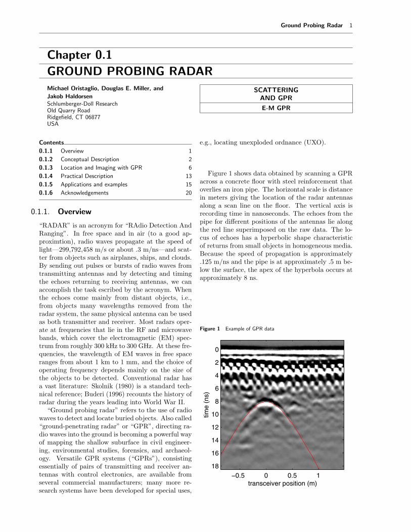
Ground Probing Radar 1

Chapter 0.1GROUND PROBING RADARMichael Oristaglio, Douglas E. Miller, andJakob HaldorsenSchlumberger-Doll ResearchOld Quarry RoadRidgefield, CT 06877USA

SCATTERINGAND GPR

E-M GPR

Contents0.1.1 Overview 10.1.2 Conceptual Description 20.1.3 Location and Imaging with GPR 60.1.4 Practical Description 130.1.5 Applications and examples 150.1.6 Acknowledgements 20

0.1.1. Overview

“RADAR” is an acronym for “RAdio Detection AndRanging”. In free space and in air (to a good ap-proximtion), radio waves propagate at the speed oflight—299,792,458 m/s or about .3 m/ns—and scat-ter from objects such as airplanes, ships, and clouds.By sending out pulses or bursts of radio waves fromtransmitting antennas and by detecting and timingthe echoes returning to receiving antennas, we canaccomplish the task escribed by the acronym. Whenthe echoes come mainly from distant objects, i.e.,from objects many wavelengths removed from theradar system, the same physical antenna can be usedas both transmitter and receiver. Most radars oper-ate at frequencies that lie in the RF and microwavebands, which cover the electromagnetic (EM) spec-trum from roughly 300 kHz to 300 GHz. At these fre-quencies, the wavelength of EM waves in free spaceranges from about 1 km to 1 mm, and the choice ofoperating frequency depends mainly on the size ofthe objects to be detected. Conventional radar hasa vast literature: Skolnik (1980) is a standard tech-nical reference; Buderi (1996) recounts the history ofradar during the years leading into World War II.“Ground probing radar” refers to the use of radio

waves to detect and locate buried objects. Also called“ground-penetrating radar” or “GPR”, directing ra-dio waves into the ground is becoming a powerful wayof mapping the shallow suburface in civil engineer-ing, environmental studies, forensics, and archaeol-ogy. Versatile GPR systems (“GPRs”), consistingessentially of pairs of transmitting and receiver an-tennas with control electronics, are available fromseveral commercial manufacturers; many more re-search systems have been developed for special uses,

e.g., locating unexploded ordnance (UXO).

Figure 1 shows data obtained by scanning a GPRacross a concrete floor with steel reinforcement thatoverlies an iron pipe. The horizontal scale is distancein meters giving the location of the radar antennasalong a scan line on the floor. The vertical axis isrecording time in nanoseconds. The echoes from thepipe for different positions of the antennas lie alongthe red line superimposed on the raw data. The lo-cus of echoes has a hyperbolic shape characteristicof returns from small objects in homogeneous media.Because the speed of propagation is approximately.125 m/ns and the pipe is at approximately .5 m be-low the surface, the apex of the hyperbola occurs atapproximately 8 ns.

Figure 1 Example of GPR data

transceiver position (m)

time

(ns)

−0.5 0 0.5 1

0

2

4

6

8

10

12

14

16

18

2 Ground Probing Radar

Figure 2 Example of 3D GPR image

By moving the surface antennas over a regularlyspaced grid of scan lines and processing the data withan imaging operator to be described below, it is pos-sible to go beyond detection and ranging to make3-D images similar to those made in X-ray tomog-raphy, magnetic-resonance imaging, medical ultra-sound, and seismic exploration. Figure 2 shows a3-D radar image of the pipe beneath the floor madefrom a dense set of scans which includes the one inFigure 1. It is natural to call this technique “ground-penetrating imaging radar” or “GPiR”.The sections that follow start with a conceptual

and mathematical description of GPR, including themost useful analytical models of radar propagation

in the ground and a simple, but rigorous, model ofradar scattering which leads to a consistent formal-ism for 3D imaging. The article concludes with abrief description of practical GPR systems and ex-amples of applications.

0.1.2. Conceptual Description

An Idealized GPR System

Figure 3 shows an idealized GPR system. It con-sists of one or more (polarized) transmitting anten-nas for broadcasting a short pulse of EM energy andone or more (polarized) receiving antennas for de-tecting the broadcast signals and their echoes. Con-trol electronics generates the current pulse which ex-cites the transmitting antenna and then samples andrecords the voltages at the receiving antennas. TheEM wave from the transmitter propagates both inthe air (direct wave) and in the earth, where it re-flects off geological structures such as changes in soillayers or man-made objects before returning to thesurface. The time of arrival of the echos is the prin-cipal source of information about buried structures.Two features distinguish GPR from other radars.

First, the antennas for transmitting and receivingGPR are roughly the same size as the spatial wave-lengths of the propagating waves. Such antennas canbe only weakly directional; therefore, precise loca-tion of a buried object with GPR requires synthetic-aperture focussing. Second, the speed of propaga-tion in the ground is significantly different from thespeed of light in free space and is not known a pri-ori. Moreover, because most soils have finite con-ductivity when wet, the wavespeed is usually com-

Figure 3 Idealized GPR system

transmitter antennasx

y

z

receiver antennas

h air

direct wave

echoes

soil

Ground Probing Radar 3

Figure 4 Electrical properties as a function of frequency for clay loams of Puerto Rico type with 2.5%, 5%, and 10% moisture content byweight (Hipp, 1974). Solid curves are experimental data; dotted curves are fits with a two-term Debye relaxation model (Wang and Oristaglio,2000).

0 100 200 300 400 500 600 700 800 900 10002

3

4

5

6

7

8

9

10 %

5 %

2.5 %

Effe

ctiv

e di

elec

tric

con

stan

t (re

lativ

e pe

rmitt

vity

)

Frequency (MHz)

0 100 200 300 400 500 600 700 800 900 1000

10-3

10-2

10-1

10 %

5%

2.5 %

Effe

ctiv

e co

nduc

tivity

(S/m

)

Frequency (MHz)

plex and varies moderately with frequency (Figure4). A complex wavespeed (or propagation constant)means that the wave decays exponentially along itspath of propagation; this limits severely the depth ofpenetration of radar signals in the ground.

Mathematical Description

GPRs generate and detect classical EM fields thatare described by Maxwell’s equations. To developsolutions relevant to GPR, we will use Cartesian co-ordinates with position vector r = xx + yy + zz,where x, y, z are unit vectors in the coordinate di-rections; R = |r| =

√x2 + y2 + z2; and r = r/R.

For fields varying harmonically in time asexp(−iωt), where ω is angular frequency, t is time,and i =

√−1, Maxwell’s equations for the electricfield E and magnetic field H are

∇ × E = iωµH, (1)

∇ × H = −iωεE + σE + Js. (2)

where the source of the EM fields is represented bythe impressed current density Js (currents on thetransmitting antenna), and the medium’s EM prop-erties are its permittivity ε, conductivity σ, and per-meability µ. In the most general anisotropic medium,these properties are all tensor functions of frequencyand position (r, ω). We will assume for simplicitythat electrical anisotropy is negligible and, morevoer,that µ assumes its free-space value µ0 = 4π × 10−7

H/m, which holds for many sandy and clay soils.The important material properties for GPR are

therefore the permittivity ε and conductivity σ,which determine the relative size of induced conduc-tion (σE) and displacement (−iωεE) currents in theground. These secondary currents—and their varia-tions caused by changes in soil or its pore fluids andby buried objects such as metallic pipe—generate the

scattered EM fields that are detected by GPR. Whenboth conduction and displacement currents are sig-nificant, it is convenient to combine them into a total(induced) current density,

JT = −iωεE + σE = −iω(ε+ iσ/ω)E (3)

and define the quantity in parenthesis as the complexpermittivity,

ε(ω) = ε(ω) + iσ(ω)/ω. (4)

There is no loss of generality in then assuming thatε and σ are (strictly) real functions, linked by therequirement that

ε(t) =1

2π

∫ ∞

−∞ε(ω) exp(−iωt)dω

be a causal function of time. One convenience of thisrepresentation is that nearly all formulas derived forlossless media (σ ≡ 0) are extended to lossy mediaby the simple substitution ε → ε.Finally is also conventional to write ε = ε0εr,

where ε0 = 8.85 × 10−12 F/m is the permittivityof free-space and εr is the medium’s relative permit-tivity, usually called its “dielectric constant”. Withthese conventions, the speed of radio waves in theground (at the operating frequencies of GPR) is de-termined mainly by n =

√εr, the index of refraction,

while the attenuation is determined by both σ andn.

Propagation, Decay, and Dispersion Maxwell’sequations (1) and (2) combine to give the vector waveequation,

∇ × ∇ × E − k2(ω)E = iωµJs, (5)

where k2 = ω2µε(ω). In regions outside the source,equation (5) has plane wave solutions of the form,

E(r, ω) ∼ Eo eik·r, (6)

4 Ground Probing Radar

where k is a complex propagation vector and Eo is acomplex amplitude vector, subject to

k · k = k2 = ω2µε(ω) ; Eo · k = 0. (7)

To simplify, assume the wave propagates along thez-axis, and is polarized along the y-direction; then

Ey(z, ω) = Eoeikz (8)

where

k = kR + ikI = ω√µε

(1 + i

σ

ωε

)1/2(9)

is the wave’s complex propagation constant and Eo

is its (real) amplitude at the surface z = 0. In gen-eral, solution (8) describes a wave which propagatesat phase velocity ω/kR and decays at the rate kI

in the positive z-direction (when kR, kI , ω > 0 andtime-dependence e−iωt is restored). Solving for thecomplex square root shows that both the speed andattenuation depend on frequency, so that radar prop-agation in conductive soil is inherently dispersive,even if ε and σ are constant with frequency.Dispersion can significantly complicate “detection

and ranging” since it changes the shapes and loca-tions of echoes. But its effects in GPR are not nec-essarily severe. Most GPRs operate at frequencieswhere displacement currents dominate, σ/(ωε) 1,and the propagation constant simplifies considerably

k ≈ ω√µε

(1 + i

σ

2ωε

)= ω/c+ iα, (10)

with

c =1√µε

=c0

nand α =

σ

2

õ

ε=η0σ

2n, (11)

where co = (µ0ε0)−1/2 is the speed of light in free-space, n =

√εr is the index of refraction, and

η0 = (µ0/ε0)1/2 ≈ 377 Ω is the impedance of free-space. In this regime, the wavespeed and the attenu-ation rate are independent of frequency if ε and σ areconstant. Pulses in this regime retain their shapes,but are attenuated exponentially along the path ofpropagation at a rate that is constant with frequency.Thus, when σ/(ωε) 1, a lower frequency GPR doesnot necessarily have increased depth of penetration.In practice, however, water in the soil does causesome variation of both ε and σ at frequencies in thebandwidth of GPR (Figure 4). The examples belowshow that this dispersion has only subtle effects onechoes from buried objects. But the higher attenua-tion caused by higher σ at higher frequencies can besignificant.Most soils have dielectric constants in the range

2-16, which means that speed of propagation in the

ground is as much as four times slower than in air,and there is significant refraction of radio waves atthe earth-air interface. Conductivity varies fromnearly zero in dry sandy soils to about .1 S/m inwet clays. Both of these properties are influencedstrongly by the amount of (salt) water saturation.(Values of conductivity are often given in terms oftheir inverse, the resistivity, ρ = 1/σ. Most soilshave resistivities in the range 10–10 000 Ω-m.)

Antennas and Sources The most popular com-mercial GPRs use either linear or bow-tie antennas(Figure 5) backed by a metal cavity containing aradar-absorbing dielectric material. Modeling thesein detail is complicated (Nishioka, et al., 1999), buttheir radiated fields are approximated well by thatof an ideal (broadband) electric dipole. The inducedsecondary currents on a small isolated object also ra-diate, to good approximation, as an equivalent elec-tric dipole (in the limit of an ideal point scatterer,this equivalence is exact).

Figure 5 GPR bow-tie antennas

Thus, the solution of the vector wave equationin a homogeneous medium where the source is apoint electric dipole in an arbitary direction—i.e.,Js = δ(r)u—is probably the most important modelin GPR.We can obtain this solution from the Green’s

dyadic for the vector wave equation, which satisfies

∇ × ∇ × Go(r, r′, ω) − ω2µεGo(r, r′, ω) = I δ(r − r′). (12)

where I = xx+yy+zz is the identity dyadic. Green’sdyadic plays the role of Green’s function for problemswith vector fields and sources. If u is a arbitrary unitvector, then

iωµGo(r, r′, ω) · u (13)

Ground Probing Radar 5

is the vector electric field at position r caused by apoint electric dipole with unit strength and directionu at position r′. In Cartesian coordinates, Green’sdyadic can be represented as a 3 × 3 matrix whosecolumns are (proportional to) the vector electric fieldcaused, respectively, by electric dipoles in the coor-dinate directions x, y, and z. A dyadic (matrix)Green’s function is needed because the field vector isnot necessarily parallel to the source vector.Green’s dyadic for a homogeneous medium has

a simple explicit form, that splits neatly into twoterms,

G(r, r′, ω) = (I + k−2∇∇)eikR

4πR

= (I − RR)eikR

4πR

+(i

kR− 1k2R2

)(I − 3RR)

eikR

4πR, (14)

where R = |r − r′|, R = (r − r′)/R, and k = ω√µε.

Positive real and imaginary parts are chosen for thesquare root to give an outgoing and decaying spheri-cal wave, with exp(−iωt) time-dependence. The firstterm, which dominates at large distances comparedto a wavelength (|kR| = 2πR/λ 1) is the radiationor far field. The dyadic factor in this term guaranteesthat its electric field is polarized perpendicular to thedirection of propagation (the radial vector from thesource). The radiation field thus locally resemblesan EM plane wave. The polarization of the near-field (second) term is the same as that of a staticelectric dipole.The transient field of the dipole is, from (13) and

(14),

E(r, t) = Re

µ

π

∫ ∞

0

iωG(r, r′, ω) · J(r′, ω)e−iωtdω

. (15)

In conductive media, the integral must be evalu-ated numerically, but it simplifies considerably whenσ = 0. If I(ω) is the dipole’s current moment (inunits of amp-m) so that J = I(ω)δ(r − r′)u, thenin the far field, the transient electric field is justthe time-derivative of the current waveform with thepropagation delay R/c,

E(r, t) ≈ (I − RR) · u µ

4πRI′(t−R/c), (R → ∞) (16)

where I ′ = dI/dt. The time-dependence of the near-field term includes a combination of the source cur-rent and its integral.In conductive soil, the wave is attenuated and

distorted significantly as it propagates, but in soilswhere ωε/σ 1 in the effective bandwidth of thesource current, the main effect in the far field is anexponential attenuation,

E(r, t) ≈ (I − RR) · uµe−αR

4πRI′(t−R/c), (R → ∞) (17)

where α = σµc/2 = ση0/(2n).Figure 6 shows the evolution from the near to far

field in a wholespace with relative dielectric εr = 9, atypical value for sandy soils, corresponding to a speedof light of .1 m/ns. Waveforms are shown for soils inwhich the conductivity increases from 0 to .05 S/m (arelatively conductive soil). The source current is thefirst derivative of a gaussian function with a centralfrequency of about 200 MHz. The wavelength in thenon-conductive soil at the central frequency of thesource is about 0.5 m. At a distance of 1.5 m from thesource—or 3 wavelengths at the central frequency—the far field approximation is already accurate to afew per cent.

Earth-Air Interface Presence of the interface be-tween earth and air is another obvious differencebetween GPR and conventional radar. Sommerfeld(1912) began the study of radio waves near the in-terface by constructing his famous integral, and ex-ploration of its subtleties remains an area of activeresearch (e.g., to determine where cellular phones willwork). Fortunately, when GPR antennas are placedclose to the ground—within a quarter wavelength orless, as in most surveys—most of these subtleties canbe ignored. The main effect of the interface on scat-tering by buried objects is a change in the radia-tion and receiving patterns of the antennas. Thiseffect is accurately modeled by asymptotic formulasfor Green’s dyadic in a halfspace. For GPR surveyswith horizontal antennas on the ground, the relevantcomponents of Green’s dyadic—the first 2 columns,corresponding to the (vector) electric fields in thehalfspace caused by x- and y-directed dipoles at theinterface—can be obtained from the formulas for thefield of a horizontal dipole at the interface (Enghetaet al., 1982). The solution is conviently written withthe dipole at the origin in spherical coordinates,

G(r, r′ = 0) ∼ e−σµcR

4πReiωR/c

[F (θ)φφ −G(θ)θ(φ × z)

](18)

where θ and φ are polar and azimuthal angles of theradius vector to point r; θ and φ are unit vectors inthe corresponding directions; and the angular factorsare

F (θ) =2n cos θ

(1 − n2 sin2 θ)1/2 + n cos θ(19)

G(θ) =2n cos θ

n(1 − n2 sin2 θ)1/2 + cos θ(1 − n2 sin2 θ)1/2, (20)

where n =√εr is the index of the refraction of the

ground.

6 Ground Probing Radar

GPR antennas close to the interface also excite astrong ground wave, which propagates at the speed ofradar waves in the soil. Thus, GPR data has two “di-rect” waves between transmitter and receiver anten-nas: one propagating in air and one in ground. Thesewaves interfere when the two antennas are close to-gether (within a wavelength or two), but separateclearly in any GPR survey in which the transmitterantenna is held fixed and the receiver is moved tosuccessive larger separations or receivers are laid outin an array at different distances from the source.

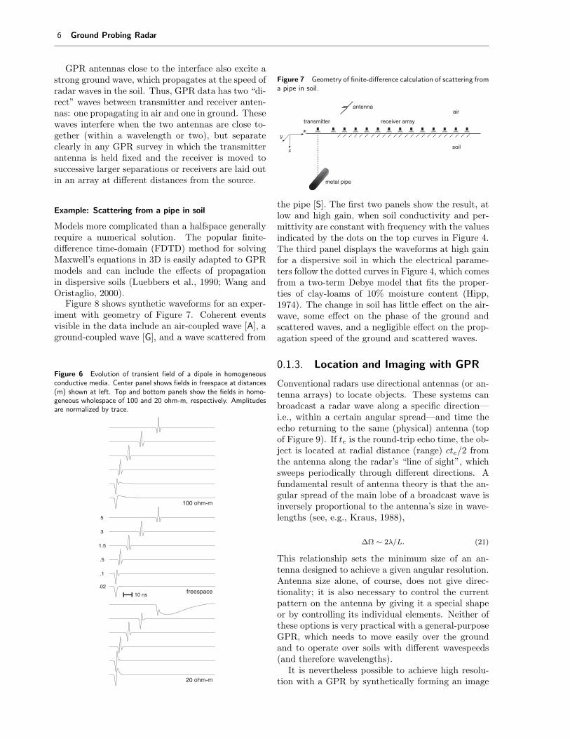
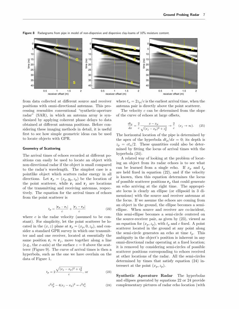
Example: Scattering from a pipe in soil

Models more complicated than a halfspace generallyrequire a numerical solution. The popular finite-difference time-domain (FDTD) method for solvingMaxwell’s equations in 3D is easily adapted to GPRmodels and can include the effects of propagationin dispersive soils (Luebbers et al., 1990; Wang andOristaglio, 2000).Figure 8 shows synthetic waveforms for an exper-

iment with geometry of Figure 7. Coherent eventsvisible in the data include an air-coupled wave [A], aground-coupled wave [G], and a wave scattered from

Figure 6 Evolution of transient field of a dipole in homogeneousconductive media. Center panel shows fields in freespace at distances(m) shown at left. Top and bottom panels show the fields in homo-geneous wholespace of 100 and 20 ohm-m, respectively. Amplitudesare normalized by trace.

.02

.1

.5

1.5

3

5

20 ohm-m

100 ohm-m

freespace10 ns

Figure 7 Geometry of finite-difference calculation of scattering froma pipe in soil.

transmitter

x

y

z

receiver array

air

soil

antenna

metal pipe

the pipe [S]. The first two panels show the result, atlow and high gain, when soil conductivity and per-mittivity are constant with frequency with the valuesindicated by the dots on the top curves in Figure 4.The third panel displays the waveforms at high gainfor a dispersive soil in which the electrical parame-ters follow the dotted curves in Figure 4, which comesfrom a two-term Debye model that fits the proper-ties of clay-loams of 10% moisture content (Hipp,1974). The change in soil has little effect on the air-wave, some effect on the phase of the ground andscattered waves, and a negligible effect on the prop-agation speed of the ground and scattered waves.

0.1.3. Location and Imaging with GPR

Conventional radars use directional antennas (or an-tenna arrays) to locate objects. These systems canbroadcast a radar wave along a specific direction—i.e., within a certain angular spread—and time theecho returning to the same (physical) antenna (topof Figure 9). If te is the round-trip echo time, the ob-ject is located at radial distance (range) cte/2 fromthe antenna along the radar’s “line of sight”, whichsweeps periodically through different directions. Afundamental result of antenna theory is that the an-gular spread of the main lobe of a broadcast wave isinversely proportional to the antenna’s size in wave-lengths (see, e.g., Kraus, 1988),

∆Ω ∼ 2λ/L. (21)

This relationship sets the minimum size of an an-tenna designed to achieve a given angular resolution.Antenna size alone, of course, does not give direc-tionality; it is also necessary to control the currentpattern on the antenna by giving it a special shapeor by controlling its individual elements. Neither ofthese options is very practical with a general-purposeGPR, which needs to move easily over the groundand to operate over soils with different wavespeeds(and therefore wavelengths).It is nevertheless possible to achieve high resolu-

tion with a GPR by synthetically forming an image

Ground Probing Radar 7

Figure 8 Radargrams from pipe in model of non-dispersive and dispersive clay-loams of 10% moisture content.

A

receiver offset (m)

time

(ns) G

S

0.5 1 1.5 2

0

5

10

15

20

25

30

35

40

G

receiver offset (m)

time

(ns)

A

S

0.5 1 1.5 2

0

5

10

15

20

25

30

35

40

G

A

S

receiver offset (m)

time

(ns)

0.5 1 1.5 2

0

5

10

15

20

25

30

35

40

from data collected at different source and receiverpositions with omni-directional antennas. This pro-cessing resembles conventional “synthetic-apertureradar” (SAR), in which an antenna array is syn-thesized by applying coherent phase delays to dataobtained at different antenna positions. Before con-sidering these imaging methods in detail, it is usefulfirst to see how simple geometric ideas can be usedto locate objects with GPR.

Geometry of Scattering

The arrival times of echoes recorded at different po-sitions can easily be used to locate an object withnon-directional radar if the object is small comparedto the radar’s wavelength. The simplest case is apointlike object which scatters radar energy in alldirections. Let rp = (xp, yp, zp) be the location ofthe point scatterer, while ri and rj are locationsof the transmitting and receiving antennas, respec-tively. The equation for the arrival times of echoesfrom the point scatterer is

tp =|rp − ri|c

+|rj − rp|c

(22)

where c is the radar velocity (assumed to be con-stant). For simplicity, let the point scatterer be lo-cated in the (x, z) plane at rp = (xp, 0, zp), and con-sider a standard GPR survey in which one transmit-ter and and one receiver, located at essentially thesame position ri ≈ rj , move together along a line(e.g., the x-axis) at the surface z = 0 above the scat-terer (Figure 9). The curve of arrival times is then ahyperbola, such as the one we have overlain on thedata of Figure 1,

tp = 2

√(xj − xp)2 + z2p

c, or (23)

c2t2p − 4(xj − xp)2 = c2t2o (24)

where to = 2zp/c is the earliest arrival time, when theantenna pair is directly above the point scatterer.The velocity c can be determined from the slope

of the curve of echoes at large offsets,

dtp

dx=

2c

x− xp√(xj − xp)2 + z2p

→ 2c

(xj → ∞). (25)

The horizontal location of the pipe is determined bythe apex of the hyperbola dtp/dx = 0; its depth iszp = cto/2. These quantities could also be deter-mined by fitting the locus of arrival times with thehyperbola (24).A related way of looking at the problem of locat-

ing an object from its radar echoes is to see whatcan be learned from a single echo. If xp and tpare held fixed in equation (22), and if the velocityis known, then this equation determines the locusof possible scatterer positions rp that could generatean echo arriving at the right time. The appropri-ate locus is clearly an ellipse (or ellipsoid in 3 di-mensions) with the source and receiver antennas atthe focus. If we assume the echoes are coming froman object in the ground, the ellipse becomes a semi-ellipse. When source and receiver are co-incident,this semi-ellipse becomes a semi-circle centered onthe source-receiver pair, as given by (23), viewed asan equation for (xp, zp), with tp and c fixed. A pointscatterer located in the ground at any point alongthe semi-circle generates an echo at time tp. Thisambiguity in the object’s position is inherent in anyomni-directional radar operating at a fixed location;it is removed by considering semi-circles of possiblescatterer positions corresponding to echoes receivedat other locations of the radar. All the semi-circlesdetermined by times that satisfy equation (24) in-teresect at the point (xp, zp).

Synthetic Aperature Radar The hyperbolasand ellipses generated by equations 22 or 24 providecomplementary pictures of radar echo location (with

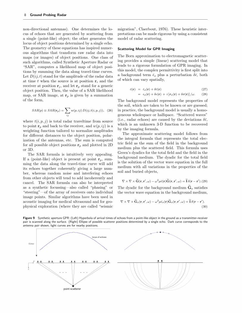
8 Ground Probing Radar

non-directional antennas). One determines the lo-cus of echoes that are generated by scattering froma single (point-like) object; the other generates thelocus of object positions determined by a single echo.The geometry of these equations has inspired numer-ous algorithms that transform raw radar data intomaps (or images) of object positions. One class ofsuch algorithms, called Synthetic Aperture Radar or“SAR”, computes a likelihood map of object posi-tions by summing the data along travel-time curves.Let D(ij, t) stand for the amplitude of the radar dataat time t when the source is at position ri and thereceiver at position rj , and let rp stand for a genericobject position. Then, the value of a SAR likelihoodmap, or SAR image, at rp is given by a summationof the form,

SAR(p) ≡ SAR(rp) =∑

ij

w(p, ij)D(ij, t(i, p, j)), (26)

where t(i, p, j) is total radar traveltime from sourceto point rp and back to the receiver, and w(p, ij) is aweighting function tailored to normalize amplitudesfor different distances to the object position, polar-ization of the antennas, etc. The sum is computedfor all possible object positions rp and plotted in 2Dor 3D.The SAR formula is intuitively very appealing.

If a (point-like) object is present at point rp, sum-ming the data along the travel-time curve will addits echoes together coherently giving a large num-ber, whereas random noise and interfering echoesfrom other objects will tend to add incoherently andcancel. The SAR formula can also be interpretedas a synthetic focussing—also called “phasing” or“steering”—of the array of receivers onto individualimage points. Similar algorithms have been used inacoustic imaging for medical ultrasound and for geo-physical exploration (where they are called “seismic

migration”, Claerbout, 1976). These heuristic inter-pretations can be made rigorous by using a consistentmodel of radar scattering.

Scattering Model for GPR Imaging

The Born approximation to electromagnetic scatter-ing provides a simple (linear) scattering model thatleads to a rigorous formulation of GPR imaging. Inthis model, the complex permittivity is first split intoa background term εo plus a perturbation δε, bothof which can vary spatially,

ε(r) = εo(r) + δε(r) (27)

= εo(r) + δε(r) + i [σo(r) + δσ(r)] /ω. (28)

The background model represents the properties ofthe soil, which are taken to be known or are guessed;in practice, the background model is usually a homo-geneous wholespace or halfspace. “Scattered waves”(i.e., radar echoes) are caused by the deviations δε,which is an unknown 3-D function to be recoveredby the imaging formula.The approximate scattering model follows from

the integral formula that represents the total elec-tric field as the sum of the field in the backgroundmedium plus the scattered field. This formula usesGreen’s dyadics for the total field and the field in thebackground medium. The dyadic for the total fieldis the solution of the vector wave equation in the fullmedium with all variations in the properties of thesoil and buried objects,

∇ × ∇ × G(r, r′, ω) − ω2µε(r)G(r, r′, ω) = I δ(r − r′).(29)

The dyadic for the background medium Go satisfiesthe vector wave equation in the background medium,

∇ × ∇ × Go(r, r′, ω) − ω2µεo(r)Go(r, r′, ω) = I δ(r − r′).(30)

Figure 9 Synthetic aperture GPR: (Left) Hyperbola of arrival times of echoes from a point-like object in the ground as a transmitter-receiverpair is scanned along the surface. (Right) Ellipse of possible scatterer positions determined by a single echo. Dark curve corresponds to theantenna pair shown; light curves are for nearby positions.

x

z

point scatterer

time

locus of echoes

Ground Probing Radar 9

These Green’s dyadics have the usual interpretation:if u is a unit vector giving the direction of a dipolesource at position r′, then iωµG(r, r′, ω) · u is thevector electric field at position r in the full medium;and iωµGo(r, r′, ω) · u is the vector electric field inthe background medium.We will assume that the transmitting antenna is

an ideal electric dipole,

Js(r) = I(ω) δ(r − rj)uj , (31)

with current moment I(ω) (amp-m) and directionuj , and that the output of the receiving antennacan be converted into a measurement of the elec-tric field. These assumptions imply that radar dataare essentially different components of the Green’sdyadic. For example, with a GPR transmitter an-tenna aligned in the x-direction at position rj anda receiver antenna aligned in the y-direction at ri

(a cross-polarized measurement), then the measuredelectric field is

iωµI(ω) y · G(ri, rj , ω) · x.

The measurement includes both the “direct” wavesin the background medium and the EM field scat-tered by buried objects. When using radar to imagethe objects, one usually subtracts an estimate of thedirect coupling between the transmitter and receiverantennas in the background medium. To model this,we use the “scattered field” dyadic, defined as the dif-ference between the total field and the backgroundfield,

Gs(r, rj , ω) ≡ G(r, rj , ω) − Go(r, rj , ω). (32)

A full set of scattered-field radar measurementsthen comprise a 3× 3 data matrix,

D(ri, rj , ω) =

Dxx Dxy Dxz

Dyx Dyy Dyz

Dzx Dzy Dzz

, (33)

where

Dyx = iωµI(ω) y · Gs(ri, rj , ω) · x, etc. (34)

With ideal dipoles as transmitters and receivers,the data matrix is symmetric because of reciprocity.Generally, only horizontal antennas are used in GPRsurveys; this gives 3 independent polarizations fromthe upper-left 2 × 2 matrix: Dxx, Dyy, and Dxy =Dyx. In what follows, we maintain the conventionthat rj represents positions of a transmitter antennaand ri positions of a receiver antenna, and will referto the Green’s dyadics as “fields”, since field compo-

nents are obtained by sandwiching the dyadics withunit vectors and multiplying by iωµI(ω).With these definitions, the scattered field has the

integral representation,

Gs(r, rj , ω) = ω2µ

∫Vs

dr′ Go(r, r′, ω) · G(r′, rj , ω)δε(r′),

(35)

in which the scattering currents, (−iωδε)(iωµG),driven by the total electric field in the scatterer, ra-diate with the background Green’s dyadic. Equation(35) is the basic integral equation for forward andinverse EM scattering. The integration is over theregion of support of the contrast function: Vs = r′ :δε(r′) = 0. The point r where the field is com-puted can be anywhere. When the contrast func-tion is known, equation (35) becomes a linear integralequation for the field by letting r range over the scat-tering region. When contrast function is unknown,as in radar imaging, equation (35) becomes a non-linear integral equation for determining δε from thescattered field recorded outside the scattering region,r = ri ∈ Vs.Inversion for δε is nonlinear because the total field

G which multiples δε in equation (35) also dependson δε. The equation is linearized by replacing thetotal field G in the integral by the background fieldGo, giving

GBs (ri, rj , ω)

= ω2µ

∫Vs

dr′ Go(ri, r′, ω) · Go(r′, rj , ω)δε(r′) (36)

= ω2µ

∫Vs

dr′ GTo (r′, ri, ω) · Go(r′, rj , ω)δε(r′). (37)

The second equation, which is perfectly symmetricin sources and receivers, follows from the symmetryof electric Green’s dyadic under (matrix) transpo-sition, GT = G (see, e.g., Felsen and Marcuvitz,1975).Equation (36) is the Born approximation for vec-

tor EM scattering (Chew, 1990). It is the only self-consistent linear relation between the scattered fieldand the perturbation δε. All linear radar imagingmethods therefore rest, explicitly or implicitly, onthe assumption that this equation accurately modelsthe actual scattered field—i.e., measured radargramswith the direct field substracted.1 The next sectiondevelops a specific and flexible formula that is basedon interpreting equation (36) as a generalized Radontransfrom. To simplify the notation in what follows,we will drop the superscripts “B” and “o” since ev-erything relies on the Born approximation and thebackground model is the only model used in imag-ing.

10 Ground Probing Radar

EM Scattering as a Generalized Radon Transform

Quantitative radar imaging requires an inversion ofequation (36) to recover δε. A general theory forinverting this and similar equations, involving theGreen’s function of wave propagation, can be de-rived from the theory of Fourier Integral Operators(Beylkin, 1985) and the generalized Radon transform(Miller et al., 1987). The ordinary Radon transformis an operator that maps a function into its integralsover straight lines in 2D or planes in 3D. Its inverse isknown explictly and provides the inversion formulasfor X-ray tomography and magnetic resonance imag-ing (Deans, 1982). The generalized Radon transform(GRT) maps a function into its weighted integralsover a family of curved surfaces. Although the GRTis invertible under general conditions, explicity for-mulas exist only for specialized surfaces—such as forintegrals over spheres (Helgason, 1984).Putting equation (36) into the form of a GRT

requires a further approximation that replaces thebackground Green’s dyadic with its high-frequencyapproximation by geometrical ray theory. Since thedevelopment of this approximation for EM fields islengthy, we will simply quote the relevant results.Details can be found in Born and Wolf (1983), Klineand Kay (1965), and Felsen and Marcuvitz (1973).Geometrical ray theory assumes that the Green’s

dyadic in the high-frequency limit can be written asthe product of a geometrical amplitude factor and anexponential (phase) factor:

G(r, r′) = A(r, r′) eiωτ(r,r′), (38)

where A is a dyadic amplitude, independent of fre-quency, and iωτ is the phase. In this representation,τ will become the traveltime along a raypath. Equa-tions for the amplitude and traveltime are developedby substituting equation (38) into (30) and takingthe limit ω → ∞. The leading-order result is theeikonal equation for the traveltime,

∇τ · ∇τ = µε(r). (39)

and the transport equation for the dyadic amplitude(outside the source region),

A∇2τ + 2∇τ A · ∇ ln ε(r) + 2(∇τ · ∇)A + σµA = 0, (40)

where ε(r) and σ(r) are the real permittivity and con-ductivity. When equations (39-40) are solved in theusual way—e.g., by tracing bundles of rays—the lastterm in equation (40) gives an additional exponentialattenuation of the amplitude,

exp

(−1

2

∫dl σ(r)µc(r)

)≡ exp

(−

∫dl α(r)

), (41)

where α(r) is the attenuation rate and the integralis along the raypath (Kline and Kay, 1965). For ex-ample, geometrical ray theory for a point dipole in ahomogeneous conducting medium gives

G(r, r′) ∼ (I − RR)e−αR

4πReiωR/c, (42)

which is just the far-field term in equation (14), withthe further approximation that σ/(ωε) 1. As dis-cussed before, the exponential attenuation in thisregime is independent of frequency and is propor-tional to the product of the conductivity and theintrinsic impedance of the medium, η =

√µ/ε.

Replacing the Green’s dyadics in equation (36)with their asymptotic forms gives

Gs(ri, rj , ω) = ω2µ

∫dr′ A(ri, r′, rj) eiωτ(ri,r′,rj) δε(r′).

(43)

where

A(ri, r′, rj) = A(ri, r′) · A(r′, rj) and (44)

τ(ri, r′, rj) = τ(ri, r′) + τ(r′, rj) (45)

are the total amplitude and total traveltime alongthe path from source to scattering point to receiver.When transformed to the time domain, this equationbecomes a generalized Radon transform in the time-domain. Consider, for example, the Dyx componentof the data at time t,

Dyx(ri, rj , t) = µ

∫ ∞

−∞dωe−iωtiω3I(ω)· (46)∫

dr′ y · A(ri, r′, rj) · x eiωτ(ri,r′,rj) ε(r′)

= −µ∂3I(t)∂t3

$

∫Vs

dr′ δ[t− τ(ri, r′, rj)

]Ayx(ri, r′, rj) δε(r′)

− µ∂2I(t)∂t2

$

∫Vs

dr′ δ[t− τ(ri, r′, rj)

]Ayx(ri, r′, rj) δσ(r′),

(47)

where % indicates a temporal convolution. The deltafunctions collapse the spatial integrals over r′ topoints that satisfy the travel-time contraint:

r′ : τ(ri, r′, rj) = τ(ri, r′) + τ(r′, rj) = t. (48)

This locus of points will generally be a curved sur-face, determined by the velocity in the backgroundmodel and the positions of the antennas. For ex-ample, when transmitter and receiver are coincidentin a homogeneous background medium ri = rj , thescattered field at successive times t involves weightedintegrals of conductivity and permittivity over largerand larger spherical surfaces,

S = r′ : 2|rj − r′|/c = t.

Ground Probing Radar 11

SAR Imaging by Inversion of the GRT

An approximate inversion of equation (47) can bederived by localizing the inversion formula for theordinary Radon transform over planes.2 In fact, it iseasiest to develop this formula working with equa-tion (43) and the spatial Fourier transformation inspherical coordinates. Our convention for the for-ward transformation is

f(κ) = f(κ, ξ) =

∫dr′ eiκ·r′

f(r′) =

∫dr′ eiκξ·r′

f(r′),

(49)

where the position vector in the Fourier domain isrepresented by 3-D spherical coordinates, κ = κξ; ξis a (radial) unit vector; and κ is the distance fromthe origin. The inverse transformation is

f(r) =1

16π3

∫dξ

∫ ∞

−∞dκκ2e−iκξ·rf(κ, ξ), (50)

where the ξ integral is over the unit sphere. (An ex-tra factor of 1/2 appears in this formula comparedto the standard Cartesian formula because integra-tion over the full unit sphere and over positive andnegative radial frequencies κ gives a double coverageof Fourier space.)In standard spherical coordinates with polar angle

θ and azimuthal angle φ,

ξ = (sinθ cosφ, sinθ sinφ, cos θ)

, and dξ = sin θ dφdθ. Substituting (49) into (50)gives

f(r) =1

16π3

∫dξ

∫ ∞

−∞dκκ2

∫dr′ e−iκξ·(r−r′)f(r′).(51)

Inversion of equation (43) involves reworking itinto a form that resembles (51). First, let

D(ri, rj , ω) ≡

Dxx

Dyx

Dxy

Dyy

and A(ri, rj , ω) ≡

Axx

Ayx

Axy

Ayy

(52)

be the data and amplitude vectors made from com-ponents of the data matrix D (equation 33) and theamplitude dyadic A. In GPR surveys with just hor-izontal antennas, equation (43) then becomes

D(ri, rj , ω) = H(ω)

∫dr′ A(ri, r′, rj) eiωτ(ri,r′,rj) δε(r′),

(53)

where H(ω) = iµ2ω3I(ω) is a (pure) frequency fac-tor. Next, assume that the contrast function is local-

ized around an arbitrary point r and thatA(ri, r′, rj)varies slowly near r,

A(ri, r′, rj) ≈ A(ri, r, rj) + ∇A · (r′ − r) ≈ A(ri, r, rj),

(54)

so that it can be approximated by its value at rand removed from the integral. Multiplying equa-tion (43) by e−iωτ(ri,r,rj) then gives

e−iωτ(ri,r,rj)D(ri, rj , ω) =

H(ω)A(ri, r, rj)

∫dr′eiω[τ(ri,r,rj)−τ(ri,r′,rj)] δε(r) + error

(55)

where the “error” term absorbs all the approxima-tions leading to this point.The right-hand side of equation (55) has the form

of a Fourier integral operator acting on the functionδε (Beylkin, 1985). Its dominant action at r as ω →∞ can be obtained from the first term of a Taylorexpansion of the phase about r,

τ(ri, r′, rj) − τ(ri, r, rj) ≈ ∇τ(ri, r, rj) ·(r′ − r

). (56)

For any given source-receiver pair, the gradient ofthe total traveltime (on the right-hand side) is thesum of the gradients of traveltimes from the sourceto point r and from point r to the receiver:

∇τ(ri, r, rj) = ∇τ(ri, r) + ∇τ(r, rj). (57)

The geometry of this vector relationship is shownin Figure 10. Since traveltime increases as r moveslocally away from the source or receiver along a ray-path, ∇τ(r, rj) points along the ray that arrives atr from the transmitter; similarly, ∇τ(ri, r) pointsalong the ray that arrives at r from the receiver. Letξ be a unit vector in the direction of the total gra-dient. It is easy to see geometrically or algebraicallythat

∇τ(ri, r, rj) =2 cosα(ri, r, rj)

c(r)ξ(ri, r, rj)

≡ s(ri, r, rj)ξ(ri, r, rj), (58)

where s ≡ |∇τ | = 2 cosα/c, and α is half the anglebetween the two rays at r. The unit vector ξ willplay the role of the Fourier-domain radial vector inthe inversion of equation (55) (by comparison withequation 51). This unit vector is connected to thesource and the receiver by the raypaths (Figure 2);thus, integration over ξ(ri, r, rj) becomes an integralover source and receiver positions.Substituting (58) into (55) gives

e−iωτ(ri,r,rj)D(ri, rj , ω) =

H(ω)A(ri, r, rj)

∫dr′eiωsξ·(r′−r)δε(r′) + error

(59)

12 Ground Probing Radar

where for simplicity we have dropped the argumentsof s and ξ. The integral term on the right-hand sidenow resembles the inversion formula (51). But sinceboth sides of this equation are vectors, it is an overde-termined system for the scalar δε. Least-squares so-lution of this system amounts to operating on it withthe pseudo-inverse of the vector A,

A+(ri, r, rj) = limε→0

(AH · A + ε

)−1AH , (60)

where ε is a real positive number and the super-script H stands for the Hermitian transpose (to ac-count for a possibly complex amplitude factor). Left-multiplying (59) by A+ and splitting δε into compo-nents gives

e−iωτ(ri,r,rj)A+(ri, r, rj ,uj) · D(ri, rj , ω)

= H(ω)

∫dr′ eiωsξ·(r−r′) [

δε(r′) + (−iω)−1δσ(r′)]

+ error

. (61)

Comparing equations (51) and (61) indicates that thefinal step in the inversion must involve an integralover ξ and frequency ω.If the experiement surrounds the scatterer—e.g.,

if antenna positions cover a sphere that contains theunknown object—then it is easy to show that bothpositive and negative spatial frequencies of the ob-ject can be recovered from data at positive temporalfrequencies ω by the mapping κ = ωsξ (see inset inFigure 10). In practice, because the data must bereal, positive temporal frequencies are the only onesavailable (the data at positive and negative tempo-ral frequencies are complex conjugates). Still, withcomplete coverage of the Fourier domain, it is possi-ble to reconstruct both δσ and δε independently, asthe real and imaginary parts of the complex functionδε. In effect, probing from both sides of the objectgives both positive and negative spatial frequencies.In typical GPR surveys, of course, the object lies ina halfspace and can only be probed from one side. Inthis geometry only positive spatial frequencies of the

Figure 10 Geometry of rays at image point

rjri

r rjrri

xy

z

Fourier domain

kx

kz

γ

object can be reconstructed, and independent recov-ery of the conductivity and the permittivity pertur-bations is not possible without further assumptions.We thus consider two separate operators: one recov-ers the permittivity when the conductivity perturba-tion is negligible; the other recovers the conductivitywhen the permittivity perturbation in negligible.Neglecting δσ first, consider the linear operator on

D,

Hε(D) =1

16π3

∫dξ s3(ri, r, rj)·∫ ∞

−∞dω ω2H−1(ω)e−iωτ(ri,r,rj)A+(ri, r, rj) · D(ri, rj , ω)

(62)

Using equation (51) and (61) (with δσ = 0) gives

Hε(D) =1

16π3

∫dξ s3

∫ ∞

−∞dω ω2eiωsξ·(r−r′) δε(r′) + error

=1

16π3

∫dξ

∫ ∞

−∞dκκ2eiκξ·(r−r′) δε(r′) + error

= 〈δε(r)〉 , (63)

where the angle brackets indicate an estimate of thequantity. The second equality above follows fromthe change of variable κ = sω. The frequency fac-tor in Hε (equation 62), ω2H−1(ω) = [µ2iωI(ω)]−1,deconvolves the spectrum of the time-derivative ofthe transmitter current. In practice, the spectrumis not be broadband and the deconvolution must beregularized.The operator for recovering δσ differs from Hε

only by the extra frequency factor (−iω),

Hσ(D) = − 116π3

∫dξ s3(ri, r, rj)·∫ ∞

−∞dω iω3H−1(ω)e−iωτ(ri,r′,rj)A+(ri, r, rj) · D(ri, rj , ω)

(64)

The frequency factor of this operator removes thespectrum of the transmitter current.

GPR Imaging in a Homogeneous Wholespace

The simplest example of the imaging formula is fora vector radar survey with co-incident pairs of an-tennas in a homogeneous background medium (thisneglects effects at the earth-air interface for a GPRsurvey). The following geometrical parameters spec-ify the experimental geometry:

rj = (xj , yj , 0), position vector of the j-th antenna pair,

R = |r − rj |, distance from rj to image point r;,

R = (r − rj)/R, unit vector from the antennas to r;,

θr,rj = polar angle between R and the z-axis, and

φr,rj = azimuthal angle between R and the x-axis,

Ground Probing Radar 13

Then, from equation (42), the amplitude vector Asplits into a scalar amplitude that depends on R anda projection vectorP that depends on only the anglesθr,rj and φr,rj ,

A(ri, r, rj) = A(R) P(θr,rj , φr,rj ), (65)

where

Pxx = x · (I − RR) · x = 1 − sin2 θr,rj cos2 φr,rj

Pyy = y · (I − RR) · y = 1 − sin2 θr,rj cos2 φr,rj

Pyx = Pxy = y · (I − RR) · x = sin2 θr,rj cosφr,rj sinφr,rj ,

andA =

116π2

e−σµcR

R2,

A straightforward calculation shows that AH · A =A2(1+cos4 θr,rj

). For this geometry, the incident andscattered rays point in the same direction: α = 0,s = 2/c, and ξ = R. The integration over ξ is easilyconverted to an integral over the antenna positions(Miller et al., 1987) with

dξ = cos θr,rj /R2 drj .

Finally, PH = PT since the projection factors arereal. Putting this all together gives

〈δε(r)〉 =8

πc3µ2

∫d2rj

cos θr,rj

1 + cos4 θr,rj

·∞∫

−∞

dω1

iωI(ω)e−2iωR/c PT (θr,rj , φr,rj ) · D(rj , ω)eσµcR

=4c3µ2

∫d2rj

cos θr,rj

1 + cos4 θr,rj

·

PT (θr,rj , φr,rj ) · D∗(rj , t = 2|r − rj |/c)eσµc|r−rj |, (66)

where D∗(rj , t) is the data deconvolved by the time-derivative of the transmitter current ∂I(t)/∂t. Theexponential amplitude factor corrects for attenuationin the background medium (geometrical spreading isimplicitly corrected by the integral over drj). In thefinal formula, we have substituted R = |r−rj |, so allgeometrical quantities are explicit. The formula forδσ is the same except that data is first deconvolvedby I(t).In practice, equation (66) is a vector stacking al-

gorithm. Let p index (discrete) image points and ijsource-receiver positions, then

IMAGE(p) =∑j

wxx(p, j)D∗xx(j, t(p, j)) +

∑j

wyy(p, j)D∗yy(j, t(p, j)) +

∑j

wxy(p, j)D∗xy(j, t(p, j)) (67)

where D∗•• is the data (appropriately filtered), t(p, j)

is the (round trip) traveltime to the image point, andthe discrete weights w•• absorbs all other factors.

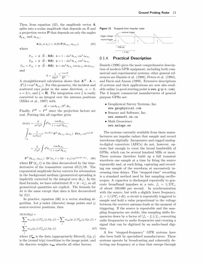
Figure 11 Stepped-time impulse radar

source trigger

receiver trigger

trigger voltage

~100 ns

~.1 ms

0.1.4. Practical Description

Daniels (1996) gives the most comprehensive descrip-tion of modern GPR equipment, including both com-mercial and experimental systems; other general ref-erences are Daniels et al. (1988), Peters et al. (1994),and Davis and Annan (1989). Extensive descriptionsof systems and their applications are now also avail-able online (a good starting point is www.g-p-r.com).The 3 largest commercial manufacturers of generalpurpose GPRs are:

• Geophysical Survey Systems, Inc.www.geophysical.com

• Sensors and Software, Inc.www.sensoft.on.ca

• Mala Geosciencewww.malags.se

The systems currently available from these manu-facturers are impulse radars that sample and recordwaveforms digitially. Inexpensive and rugged analog-to-digital converters (ADCs) do not, however, op-erate fast enough to cover the broad bandwidth ofGPRs, which can be several hundred MHz or more.These systems therefore build up a full transientwaveform one sample at a time by firing the sourcerepeatedly and, at each firing, capturing and record-ing one sample of the waveform at successively in-creasing time delays. This “stepped-time” recordingis a standard method used by fast sampling oscillo-scopes: A capacitor is discharged repeatedly to gen-erate broadband impulses at a rate, fs = 1/DTs,of about 100,000 per second. In synchronizationwith the source, but with a slightly lower frequency,fr = 1/(DTs+dt), a circuit is repeatedly triggered tosample and hold a value proportional to the voltagebetween the receiver antenna leads at the moment oftriggering. If the source is repeatable and the sam-pling frequencies are stable, this sampling shifts fre-quencies down by a factor of (fs −fr)/fr, convertingradio frequencies to audio frequencies and creating asignal that can be digitized by an audio-band digi-tizer.A few “stepped-frequency” GPR systems have

also been built by specialized manufacturers. Thesesystems operate by broadcasting and coherently de-tecting one frequency at a time that sweeps through

14 Ground Probing Radar

the GPR bandwidth. In principle, stepped-time andstepped-frequency systems are equivalent through aFourier Transform, provided the source is perfectlyrepeatable and the noise is stationary. Of course,neither condition holds exactly.

Digital impulse radars

A generic digital impulse radar uses the followingcomponents:

• A trigger generator,• A source antenna, with associated pulserelectronics,

• A receiver antenna, with associated sam-pling electronics,

• An ADC connected to a storage device(often a laptop computer).

The last three components are all configured to besynchronized by signals from the trigger generator.The trigger system generally works by first generat-ing an accurate and stable sawtooth wave (Figure11) that repeats at audio frequencies (10-100 kHz)and has a precise slope = ∆V/∆t on its trailing edge.Conceptually, this sawtooth wave itself could be usedto synchronize source and receiver electronics. Forexample, the source can be set to fire at the initialjump of the sawtooth (from 0 to 1), while the re-ceiver electronics can be set to capture and digitizea sample (of the voltage across its antenna leads)when the trailing slope of the sawtooth fails below acertain voltage vR. Decreasing this receiver triggervoltage by a fraction ∆vR on successive firings delayssuccessive samples in time by ∆t = ∆vR/slope.In practice, separate square-wave triggers for the

source and receiver electronics are usually createdfrom the sawtooth using a digital-to-analog convertorand a comparator3 by a loop of the form:

isv=VSirv=VR0For is=1:NSAMPirv=irv-deltaV_R;rtrig=COMP(sawtooth,D2A(irv));strig=COMP(sawtooth,D2A(isv));

END

In this scheme, the length of the “on” (1) intervalin the train of square waves sent to the source elec-tronics has a fixed length, whereas this interval grad-ually increases in length with each successive wavein the train sent to the receiver electronics. An ad-vantage of sending square waves is that their binarynature can allow more accurate detection of the trig-ger time. Also, the leading pulse of the square wave(“on”) can signal the electronics to prepare for ac-

tion that is triggered by the trailing edge (“off”).Obviously, any distortion of these trigger pulses cancause a loss of samples or variations in their timing.With modern electronics, however, the timing can beaccurate to hundredths of a nanosecond.

Antennas

The antennas of impulse GPRs are generally linearor bow-tie antennas designed to radiate and receiveas broadband dipoles (Figure 5). The central fre-quency of a bow-tie antenna is inversely proportionalto its length, so a 250 MHz antenna will be twice aslong (and occupy 8 times the volume) as a 500 MHzantenna. (A bow-tie antenna with a spectrum veryclose to the one shown in Figure 6 has a length of 25cm.) To minimize ringing, the ends of the antennasare resistively loaded (Shlager, et al., 1994). Anten-nas in newer systems are also surrounded with radarabsorbing material and placed in a rectangular metalcavity to minimize radiation into the air.The source electronics consist of a capacitor (or

cascading set of capacitors) that discharge throughavalanche transistors at the trigger signal. Consis-tency of source signatures depends on the manufac-turers’ abilities to control variations in the chargeand discharge cycle as temperature, moisture, orother environmental factors vary. Most systems needsome warmup time before use.The receiver electronics consists of a sampler

whose input leads are connected to the voltage gap inthe receiving antenna. When triggered, the samplervoltage jumps to a value proportional to the volt-age difference at the gap and holds that value longenough for an ADC operating at kHz frequencies todigitize and record the signal.

Digitization

The voltage sampled at the receiver is not very dif-ferent from the voltage on an audio microphone. Apreamplifier close to the receiver boosts the signal toa level suitable for digitization by an ADC similar tothose used for digitizing audio. Depending on the ageof the system design, the data will be digitized to anaccuracey from twelve to twenty bits. Time-varinggain can be applied before digitization to compensatefor limitations in bit length. Gain applied after dig-itization cannot improve signal-to-noise ratios, butmay be part of the digital signal processing chain.The digitized data is generally stored directly to aPC, which is either a dedicated device or a consumerlaptop.

Ground Probing Radar 15

Figure 12 Lab Survey Location

0.1.5. Applications and examples

The following examples from the authors’ files illus-trate cases where 3-D GPR imaging proved useful.The scanning system used in the last two exampleswas developed in a project on ground-penetratingimaging radar partly funded by the Electric PowerResearch Institute (EPRI) and the Gas Research In-stitute (GRI).

Laboratory Floor

In March 1997, the facilities manager at Schlumberger-Doll Research asked if a ground-penetrating radarsurvey could show structures beneath the floor of labworkshop where a new elevator was being planned.The location is shown in Figure 12. A floor drainjust outside the door visible in the figure suggestedthat pipes might lie under the floor.We collected 2 multi-polarization 3D GPR surveys

using a set of linear-dipole antennas with nominalfrequency of 900 MHz. The data were collected withan antenna separation of .17 m, on a regular 2-D gridwith an inline sampling rate of one trace every 0.02m and a crossline sampling of one line every 0.04 m.The rail system visible in Figure 12 was used to guidethe equipment and to control the crossline spacing. Astring, fixed at one side of the rail, was used to triggerthe pulse every 0.02 m. We collected three data setsin which source and receiver dipoles were respectivelyparallel to each other and perpendicular to the line ofacquisition (TE), parallel to each other and parallelto the line of acquisition (TM), and perpendicular toeach other (X).The data were processed using a version of the

algorithm in equation 66. Figure 13 shows the im-age volume rendered in a way to show low-amplitude

returns from the near subsurface. The regular gridpattern is understood to be the image of a steel re-inforcement mesh.

Figure 13 3D GPR image

Figure 2 shows the image volume rendered as anisosurface at a relatively high amplitude value. Inthis display we see a clear image of a pair of pipesjoind by a standard 45-degree fitting. Figure 14shows a horizontal projection of the image, overlainby a copy of the building plans drawn in 1955. Theplanned pipe location runs through a region wherethe GPR image shows an anomaly. This anomalycould be caused by bedrock whose presence causedthe builders to deviate from the plans.

Figure 14 Projection of GPR image combined with floor plan.

16 Ground Probing Radar

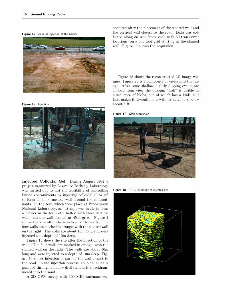
Figure 15 Zone of injection of the barrier

Figure 16 Injection

Injected Colloidal Gel During August 1997 aproject organized by Lawrence Berkeley Laboratorywas carried out to test the feasibility of controllingburied contaminents by injecting colloidal silica gelto form an impermeable wall around the contami-nants. In the test, which took place at BrookhavenNational Laboratory, an attempt was made to forma barrier in the form of a half-V with three verticalwalls and one wall slanted at 45 degrees. Figure 1shows the site after the injection of the walls. Thefour walls are marked in orange, with the slanted wallon the right. The walls are about 10m long and wereinjected to a depth of 10m deep.Figure 15 shows the site after the injection of the

walls. The four walls are marked in orange, with theslanted wall on the right. The walls are about 10mlong and were injected to a depth of 10m deep. Fig-ure 16 shows injection of part of the wall closest tothe road. In the injection process, colloidal silica ispumped through a hollow drill stem as it is jackham-mered into the sand.A 3D GPR survey with 100 MHz antennas was

acquired after the placement of the slanted wall andthe vertical wall closest to the road. Data was col-lected along 35 scan lines, each with 60 transceiverlocations, on a one foot grid starting at the slantedwall. Figure 17 shows the acquistion.

Figure 18 shows the reconstructed 3D image vol-ume. Figure 20 is a composite of views into the im-age. After some shallow slightly dipping events areclipped from view the dipping “wall” is visible asa sequence of blobs, one of which has a kink in itthat makes it discontinuous with its neighbors belowabout 5 ft.

Figure 17 GPR acquisition

Figure 18 3D GPiR Image of injected gel

Ground Probing Radar 17

Figure 20 3D images of gel

Figure 19 Survey at rock quarry

Monitoring fluids in a porous rock

In 1999 a survey was made at a rock quarry in Port-land, Connecticut, to test if time-lapse 3D GPiRcould monitor the flow of fluid injected into a porousrock. Figure 19 shows the setup: Two pairs of 400MHz antennas (“A” in Figure 19) were scanned ona motorized, computer-controlled frame over a .05 mgrid covering an area roughly 2.5 m by 2.5 m. A bore-hole 3 m long (“B” in Figure 19) was drilled at anoblique angle to the scan directions. During a two-hour period, eight surveys were made while salinebrine was injected into the rock from the packed-offend of the borehole. Data from a baseline surveywere subtracted from each successive survey and aseries of 3-D images were created.Figure 21 shows frames taken at 20, 50, and 80

minutes after start of the injection. The left panelshows the frames in 3-D perspective; the right panelshows the same images projected onto a photographof the rock surface. The borehole was imaged inde-pendently and appears in red in the left panel, yel-low in the right panel. It is evident that the fluidfound its way to a high-permeability bedding surfacewithin the sandstone and flowed mainly toward therock face lying at the right edge of the images in

18 Ground Probing Radar

Figure 21 GPiR images at 30 minute intervals

Figure 21. Figure 22 show a photo of the brine as itemerged from the rock. An arrow marks the locationwhere the first fluid emerged. It lies directly in linewith the flow seen in Figure 22.

Ground Probing Radar 19

Figure 22 Injected fluid emerging from rock

20 Ground Probing Radar

0.1.6. Acknowledgements

Notes1. Accuracy of the Born and related approximations, such as

the Rytov approximation, are the subject of a large andcontroversial literature (see, e.g., Oristaglio, 1985). It isdifficult to state precisely all the condtions under which theBorn approximation is accurate, but it is certainly accurateunder the condition that the scattered field is small (point-wise) compared to the incident field inside the scatteringvolume.

2. Norton and Linzer (1978) first derived a scalar versionof equation (47) for pulse-echo imaging (medical ultra-sound) in a homogeneous background medium and recog-nized its connection with the generalized Radon transformover spheres. They derived an exact inversion formula forthis specific GRT in the spatial Fourier transform domain.Miller et al. (1987) developed the general form of this equa-tion for acoustic imaging and derived a simple approximateinversion formula by localizing the formula for inversion ofthe standard Radon transform. Beylkin (1985) provided ajustification for this approximate formula through the the-ory of Fourier Integral Operators.

3. A comparator, COMP(a,b), is a component that gives anoutput voltage equal 1 when a > b, 0 otherwise

References1. Beylkin, G., 1985, Imaging of discontinuities in the inverse

scattering problem by inversion of a causal generalizedRadon transform, J. Math. Phys., 26, 99–108.

2. Buderi, R., 1996, The Invention that Changed the World,Simon and Schuster.

3. Born, M., and Wolf, E., 1999, Principles of Optics, 7th ed.,Cambridge U. Press.

4. Chew, W., 1990, Waves and Fields in Inhomogeneous Me-dia, Van Nostrand, New York.

5. Claerbout, J.F., 1976, Fundamentals of Geophysical DataProcessing, McGraw-Hill, New York.

6. Daniels, D. J., 1996, Surface-Penetrating Radar: Institu-tion of Electrical Engineers, London.

7. Deans, S. R., 1983, The Radon transform and some of itsapplications, J. Wiley & Sons, New York.

8. Daniels, D.J., Gunton, D.J., and Scott, H.F., 1988, Intro-duction to subsurface radar, IEE Proc., 135, 278–320.

9. Davis, J.L., and Annan, A.P., 1989, Ground-penetratingradar for high-resolution mapping of soil and rock stratig-raphy: Geophys. Prospect., 37, 531–551.

10. Engheta, N., and Papas, C.H., 1982, Radiation patterns ofinterfacial dipole antennas: Radio Science, 17, 1557–1566.

11. Felsen, L., and Marcuvitz, N., 1973, Radiation and Scat-tering of Waves, Prentice-Hall.

12. Helgason, S., 1984, Groups and geometric analysis: Inte-gral geometry, invariant differential forms, and sphericalfunctions, Academic Press.

13. Hipp, J. E., 1974, Soil electromagnetic parameters as func-tions of frequency, soil density, and soil moisture: Proc.IEEE, 62, 98–103.

14. Kline, M., and Kay, M., 1965, Electromagnetic theory andgeometrical optics, Krieger.

15. Kraus, J. D., 1988, Antennas, 2nd ed., McGraw-Hill.

16. Luebbers, R., Hunsberger, F.P., Junz, K.S., Standler, R.B.,and Schneider, M., 1990, A frequency-dependent finite-difference time-domain formulation for dispersive materi-als: IEEE Trans. Electromag. Compat., 32, 222–227.

17. Miller, D., Oristaglio, M., and Beylkin, G., 1987, A newslant on seismic imaging: Migration and integral geometry,Geophysics, 53, 943–964.

18. Oristaglio, M. L., 1985, Accuracy of the Born and Rytovapproximations for the case of refraction and reflection ata plane interface, J. Optical Soc. America A, Optics andImage Science, 2, 1987–1993.

19. Nishioka, Y., Maeshima, O., Uno, T., and Adachi, S., 1999,Three-dimensional FDTD analysis of resistor-loaded bow-tie antennas covered with ferrite-coated conducting cav-ity for subsurface radar, IEEE Trans. Ant. Propagat., 47,970–977.

20. Norton, S.G., and Linzer, M., 1981, Ultrasonic scatteringpotential imaging in three dimensions: Exact inverse scat-tering algorithms for plane, cylindrical, and spherical aper-tures, IEEE Trans. Biomed. Eng., BME-28, 202–220.

21. Peters, L., Jr, Daniels, J. J., and Young, J. D., 1994,Ground penetrating radar as a subsurface environmentalsensing tool: Proc. IEEE, 82 (Special Issue on RemoteSensing of the Environment), 1802–1822.

22. Shlager, K.L., Smith, G.S., and Maloney, J.G., 1994, Op-timization of bow-tie antennas for pulse radiation, IEEETrans. Ant. Propagat., 42, 975–982.

23. Skolnik, M. I., 1980, Introduction to radar systems, 2nded., McGraw-Hill.

24. Wang, T., and Oristaglio, M., 2000, Simulation of GPRsurveys over pipes in dispersive soils, to appear in Geo-physics.

25. Wang, T., and Oristaglio, M., 2000, GPR imaging by gen-eralized Radon transform, to appear in Geophysics.