Chapter 1 Introduction 1.1 Classification of Phase Transitions The study of phase transitions is one of the well developed branches of condensed matter physics [I]. A phase transition'.occurs when the properties of a material undergo a change due to changes in temperature or pressure. Examples of phase transitions are melting of a solid and boiling of a liquid. Transitions can also occur between phases in the solid state. An example of such a transition is the transfor- mation of a ferromagnetic substance like Iron or Nickel into a paramagnetic state. Elements like Iron and Nickel, possess permanent magnetic moments, which align spontaneously, below the transition temperature known as the Curie temperature. As the temperature of the material is increased, the degree of this alignment de- creases continuously until at the Curie temperature it becomes zero. The stability of a phase is discusied in terms of the Gibbs free energy (G) of the system. Where U = Internal energy of the system T = Temperature S = Entropy P = Pressure V = Volume In the presence of a magnetic field, a term MH is added to the Gibbs free energy .
Transcript
Chapter 1
Introduction
1.1 Classification o f Phase Transitions
The study of phase transitions is one of the well developed branches of condensed
matter physics [I]. A phase transition'.occurs when the properties of a material
undergo a change due to changes in temperature or pressure. Examples of phase
transitions are melting of a solid and boiling of a liquid. Transitions can also occur
between phases in the solid state. An example of such a transition is the transfor-
mation of a ferromagnetic substance like Iron or Nickel into a paramagnetic state.
Elements like Iron and Nickel, possess permanent magnetic moments, which align
spontaneously, below the transition temperature known as the Curie temperature.
As the temperature of the material is increased, the degree of this alignment de-
creases continuously until at the Curie temperature it becomes zero.
The stability of a phase is discusied in terms of the Gibbs free energy (G) of
the system.
Where U = Internal energy of the system
T = Temperature
S = Entropy
P = Pressure
V = Volume
In the presence of a magnetic field, a term MH is added to the Gibbs free
energy .
Chapter 1 2
For an infinitesimal , reversible transition,
dG = dU - TdS - SdT + PdV + VdP (1.2)
Using the first law of thermodynamics
TdS = dU + PdV (1.3)
Therefore
dG = -SdT + VdP
Since at the transition point the system is in thermodynamic equilibrium, d T = d P
= 0 Hence dG = 0 or G = constant a t the transition.
Even though the Gibbs free energy is a constant during a phase transition the
derivatives of the free energy like volume, entropy, specific heat, compressibility or
susceptibility can show a discontinuity a t the transition point.
The discontinuities in the various thermodynamic quantities is the basis for a
system of classifying phase transitions. According to this system of classification,
propounded by Ehrenfest [2], phase transitions are classified according to the lowest
derivative of the free energy which shows a discontinuity. If the first derivative of
the free energy i.e, either the volume or the entropy shows a discontinuity a t the
transition temperature , then it is known as a first order transition. Examples of
first order transitions are melting of a solid and boiling of a liquid.
If the second derivative of thy free energy i.e, one of the response functions like
specific heat, susceptibility etc show a discontinuity, it is known as a second order
transition. An example of a second order transition is the transition from the normal
metallic state to the superconducting state in zero magnetic field.
This system of classification fails for certain transitions , like the case of the
Curie point transition in uniaxial ferromagnets, where the second derivatives of
the free energy diverge to infinity. Hence it is difficult to see whether there is a
discontinuity or not. The modern classification of phase transitions due to Fisher,
takes this into account and broadly classifies phase transitions into discontinuous or
continuous transitions.
1.2 Theories of Phase Transitions
In this thesis we will concentrate on magnetic transitions. The earliest theory for
the ferromagnetic to paramagnetic transition was given by Weiss in 1908. According
Chapter 1 3
to this theory each atom is assumed to have a localized magnetic moment which
interacts with an average 'molecular' magnetic field due to all the other moments.
L.D.Landau, in 1944, generalized all the previous theories of phase transitions
and gave a general formulation which is known as Landau's Mean field theory. Lan-
dau used a concept known as the order parameter, first introduced by Felix Bloch.
The order parameter has a non-zero value below the transition temperature and is
zero above the transition temperature. The order parameter varies discontinuously
in a first order transition and goes continuously to zero for a continuous transition.
The main idea in Landau theory is that the free energy of the system can be
expanded as a series in the order parameter [3].
Where Go is a constant. Eq. 1.5 is written under the assumption that the value
of the order parameter is small near the transition temperature. Hence it should
be valid for continuous phase transitions. The most general expression for the free
energy would involve all possible powers of M . However it can be proved from simple
symmetry considerations that most of them should be absent. Since the free energy
is a minimum at equilibrium, dG/dM = 0. From this condition it is seen that the
coefficient of the linear term is zero. For magnetic systems, there are additional
constraints on Free energy from the symmetry consideration that G(M) = G(-M).
This is because the free energy should be the same , irrespective of the direction of
magnetization. Therefore terms containing odd powers of M are absent from the
expression for the free energy. In case the symmetry permits the presence of a term
containing M3, it can be shown that this leads to a first order transition. A first
order transition is also possible without the M3 term, if 'b' becomes negative. To
ensure stability, a term containing M6 has to be included in Eq. 1.5. For such a
system, the transition is first order when b < 0, and second order when b > 0. The
point where a = b = 0 is known as a 'tricritical point'. This shows that magnetic
transitions can also be first order under certain circumstances
The following form is usually assumed for the constant 'a'
It is obvious from the above equation that 'a' has a negative sign for T < T,
and a positive sign for T > T,. A and b are constants independent of temperature,
except under the circumstances discussed earlier.
Chapter 1
I I - 1;s -1 0 -5 0 5 10 15 order parameter
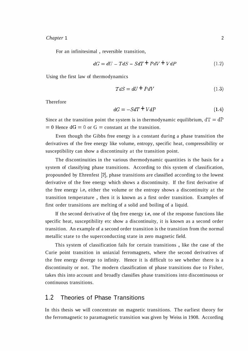
Figure 1.1: The Landau free energy as a function of the order parameter a t different temperatures
The equilibrium configuration of a system is found by minimizing the free en-
ergy with respect to variations in the order parameter. Therefore the condition for
equilibrium is that dG/dM = 0, i.e, ..
This equation has the solution M = 0 or
Therefore according to Landau theory the order parameter varies as (T -T,)'/'.
The free energy has been plotted as a function of the order parameter for different
values of temperature in Fig. 1.1.
Below T,, the free energy has two minima, corresponding to the two equivalent
directions of magnetization, -M and M. Above T,, there is only one minima a t
M = 0. As T approaches Tc from the low temperature side, the two minima ap-
proach each other and coalesce to a single point for T = Tc. Near T,, the free energy
curve is almost flat around the minima (M = 0). This brings into focus why fluctu-
Chapter 1 5
ations in the order parameter are important especially near T,. All thermodynamic
quantities are usually macroscopic quantities which are obtained by averaging over
macroscopic dimensions. There could be fluctuations on a microscopic length scale.
These fluctuations in the order parameter cost energy which depends on the size of
the fluctuation. The energy for the fluctuations are supplied by the Auctuations in
the thermal energy of the system. The effect of fluctuations are neglected in the
Landau theory based on Eq. 1.5.
To illustrate the effects of these fluctuations consider the free energy curve for
a temperature T slightly above T,. The average value of the order parameter is 0,
however fluctuations about this average value do not cost much energy as the curve
is almost flat. Hence the energy of the system is almost the same for a range of
M values about the average. his situation is no longer true far away from the
transition point, where the curvature ab,the minima of the energy is quite large,
leading to a large energy change for the same amount of fluctuation in the order
parameter. \
From the above discussion it emerges that a large number of states have the
same energy, when the system is near the transition point. This in turn means that
a long time is required for the system to attain equilibrium, as it has to sample all
the available states. This phenomenon is known as 'critical slowing7 down of the
system near the transition point. The 'critical slowing down' of the system creates
some experimental problems when a thermodynamic property has to be measured,
as the experimental time-scales diverge near the transition point.
The Landau theory ,like the Weiss theory of ferromagnetism, predicts a discon-
tinuity (AC,) in the specific heat
Experimental studies on ferromagnetic materials showed that while the mean field
theories were successful in predicting the behaviour far from the transition temper-
ature, it fails quite dramatically in its prediction near the transition temperature.
While the mean field theories predict only a discontinuity in the specific heat, fer-
romagnetic materials like Iron and Nickel show a finite cusp and some fluids show
an infinite divergence. The experimentally observed specific heat variation can be
fitted to a power-law of the form
Where Tc is the transition temperature and a is known as the critical exponent.
Chapter 1 6
The failure of the mean field theories to predict the behaviour near the transition
point is related to the fact that the theory assumes an average field throughout the
sample and neglects short-range interactions. The Ginzburg-Landau formulation
tries to rectify this defect by taking fluctuations into account.
The Ginzburg - Landau free energy is given by
The renormalization group theory of K.G.Wilson [4] uses this free energy to calculate
the variation of thermodynamic quantities near the critical temperature. It gives
values for the critical exponents which agree quite well with the experimentally
observed values of the critical exponents.
An important triumph of the renor~alizat ion group theory is the expIanation
of the phenomenon of 'universality', i.e, the explanation of the fact that many di-
verse systems give rise to the same critical exponents, even though their critical
temperatures maybe different.
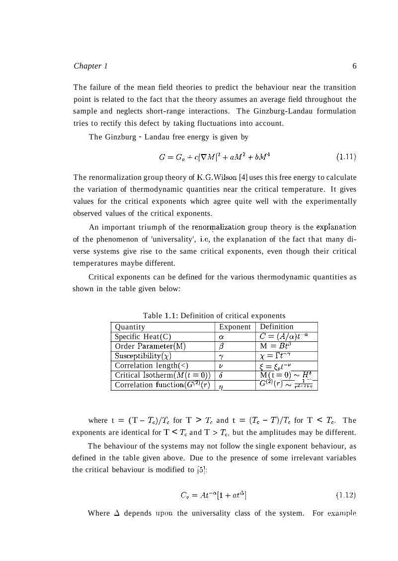
Critical exponents can be defined for the various thermodynamic quantities as
shown in the table given below:
Table 1.1: Definition of critical exponents
where t = (T - Tc)/Tc for T > T, and t = (T, - T)/T, for T < T,. The
exponents are identical for T < T, and T > T,, but the amplitudes may be different.
The behaviour of the systems may not follow the single exponent behaviour, as
defined in the table given above. Due to the presence of some irrelevant variables
the critical behaviour is modified to [5]:
Where A depends upon the universality class of the system. For exarnple
Definition C' = (A/a) t fa M = Btp x = rt-7 < = tpt-" M ( t = 0) N Hd G(')(T) &
Quantity Specific Heat (C) Order Parameter(M) Susceptibility(~) Correlation length(<) Critical Isotherm(M(t = 0)) Correlation function(G(')(r)
Exponent a P Y v S 77
Chapter 1 7
A N 0.55 for the 3d Heisenberg model. An example for an irrelevant variable is the
anisotropy in magnetic systems.
1.3 Theoretical models for Ferromagnetic systems
One of the simplest microscopic Hamiltonians to describe magnetic interactions is
the Ising model Hamiltonian. The Ising model describes the interactions between
spins localized on a lattice. The spins are allowed to be either parallel or anti-parallel
to each other. The Hamiltonian for the magnetic interaction is given by
Where Jij is the strength of the interaction between the spins Si and Sj . The spins
are assumed to be localized a t the lattice sites i and j respectively. In the case of
the Ising model, the spins a t each lattice site can only assume the values -1 or + I
,i.e, there are only two permitted directions for the spins. This corresponds to the
behaviour of a spin 112 particle. If the spins can orient along any direction in a
plane, the corresponding model is known as the XY model. If the spin can orient in
any direction in 3 dimensions, then it is described by the Heisenberg model.
It is found that the critical behaviour of the ferromagnetic metals like Iron and
Nickel are adequately described by the Heisenberg model even though the model
assumes the spins to be localized on the lattice sites. As is well known [6 ] , the
electrons contributing to the magnetic moment in the case of Nickel are itinerant
in character. This is an example of the phenomenon of universality, i.e, the insen-
sitivity of the critical behaviour to the details of the interaction Hamiltonian. The
critical exponents seem to depend only on the spatial dimension and the number of
components of the order parameter.
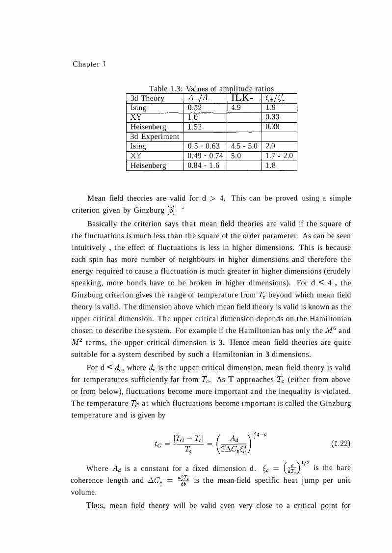
The values of the critical exponents and the amplitude ratios A+/A-for different
space and spin dimensions are given in table 1.1 and table 1.3 respectively. Where
A+ and A- are the amplitudes for the various thermodynamic quantities above and
below T,.
The tricritical point mentioned in table. 1.2 is the point a t which a transition
changes over from a first order to a second order transition. In the above table,
the exponents for 2d XY and Heisenberg models are not given since it has been
proved that a 2 dimensional system having an order parameter with more t,han one
component does not have a transition a t a finite temperature [7].
Since the determination of the exponent for specific heat will be dealt with in
Chapter 1
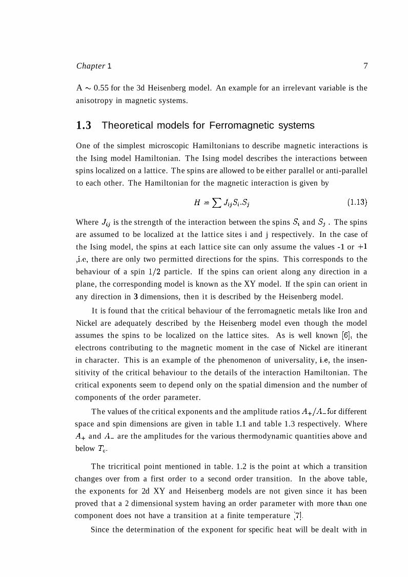
Table 1.2: Values of Critical exponents for different universality classes
- - - -
I 3d Heisenbere 1 -0.12 0.36 1 1.39 1 0.71 I I I
1 Model I Q 14 Ir Y
0.63
1 I ' I
later chapters, a few remarks on the Val& of this exponent for different models are
" tricriticalpt Mean Field Ex~er iment
in order. In the case of the 2d Ising model, the specific heat diverges as
1.24 2d Ising 3d Ising
C, = A log t (1.14)
0.5 0
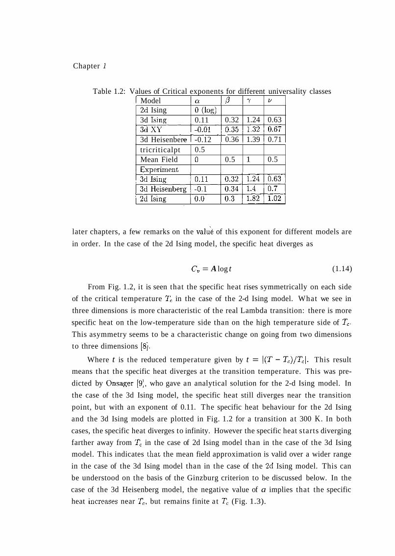
From Fig. 1.2, it is seen that the specific heat rises symmetrically on each side
of the critical temperature T, in the case of the 2-d Ising model. What we see in
three dimensions is more characteristic of the real Lambda transition: there is more
specific heat on the low-temperature side than on the high temperature side of T,.
This asymmetry seems to be a characteristic change on going from two dimensions
to three dimensions [8].
Where t is the reduced temperature given by t = I(T - T,)/T,I. This result
means that the specific heat diverges a t the transition temperature. This was pre-
dicted by Onsager [9], who gave an analytical solution for the 2-d Ising model. In
the case of the 3d Ising model, the specific heat still diverges near the transition
point, but with an exponent of 0.11. The specific heat behaviour for the 2d Ising
and the 3d Ising models are plotted in Fig. 1.2 for a transition a t 300 K. In both
cases, the specific heat diverges to infinity. However the specific heat starts diverging
farther away from Tc in the case of 2d Ising model than in the case of the 3d Ising
model. This indicates that the mean field approximation is valid over a wider range
in the case of the 3d Ising model than in the case of the 2d Ising model. This can
be understood on the basis of the Ginzburg criterion to be discussed below. In the
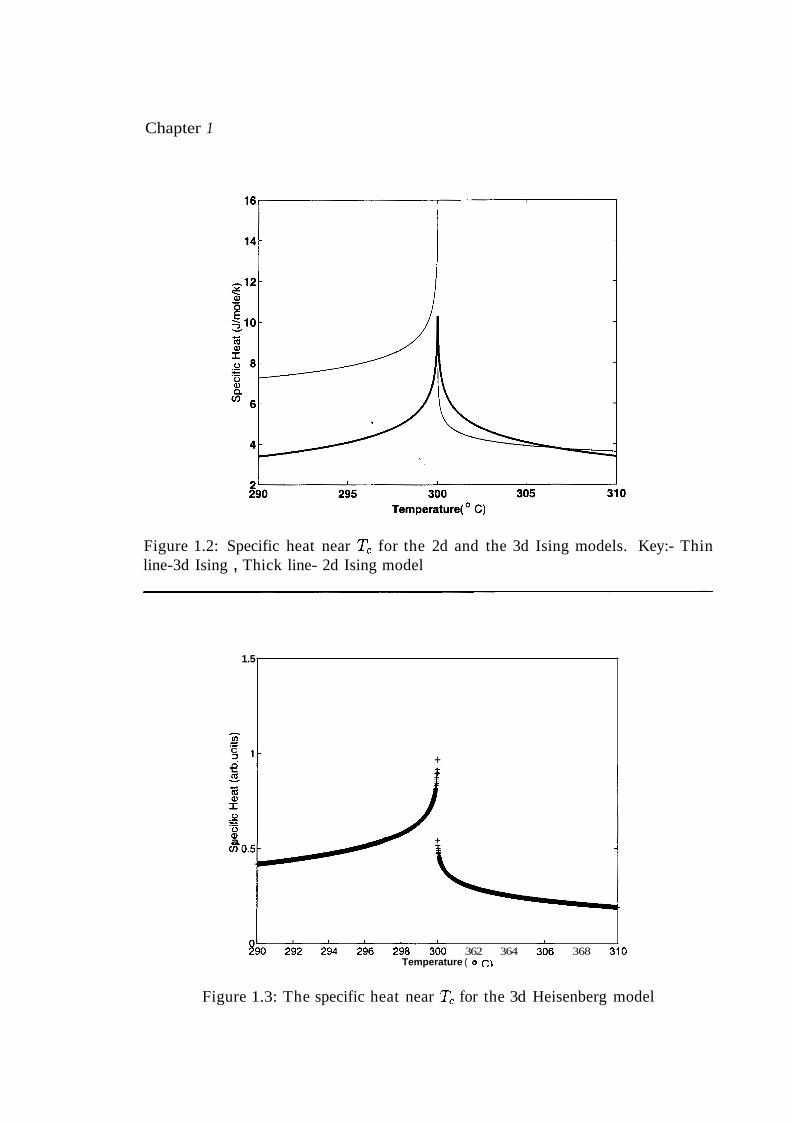
case of the 3d Heisenberg model, the negative value of a implies that the specific
heat iricreases near Tc, but remains finite a t T, (Fig. 1.3).
0 (log) 0.11 0.32
I 1
0.5 1 0.5
Chapter 1
Figure 1.2: Specific heat near Tc for the 2d and the 3d Ising models. Key:- Thin line-3d Ising , Thick line- 2d Ising model
Figure 1.3: The specific heat near Tc for the 3d Heisenberg model
1.5
- V) - .- C ? ' - +
C m
U .- *- 0 a, a
890 2 i 2 294 2 k i 300 362 364 366 368 310 Temperature ( o c)
Chapter 1 10
The difference in the behaviour of the Ising and the Heisenberg models can
be understood in a qualitative way. In the case of the Ising model, the internal
energy changes by 4NJS2 for the reversal of each spin [lo]. N is the number of spins
with which each spin interacts. If 'x' spins reverse direction for unit temperature
rise, then the change in the internal energy per unit temperature rise (which is the
specific heat) is
Now N diverges near Tc, since the correlation length J, diverges. N will roughly
go as Jd (where d is the space dimension). From the above argument it is obvious
that the specific heat will diverge in this case because of the divergence in the
correlation length.
In the case of the Heisenberg model, the above argument gets slightly modified
as the spins can point in any direction, unlike the case of the Ising model where
they can only be either parallel or anti-parallel to each other. Therefore Eq. 1.15 is
modified to
Where cos(0) is the angle between the interacting spins. As Tc is approached,
N goes to infinity, but cos(0) goes to zero (as on the average no two spins will be
aligned in the same direction), hence the product of the two can be a finite quantity.
Experimentally, it is very difficult to distinguish between the Ising and Heisen-
berg models. This is because of the fact that, even though theoretically, the specific
heat goes to infinity a t Tc in the case of the Ising model, the experimentally measured
specific heat remains finite. The experimentally measured specific heat remains fi-
nite as we cannot approach arbitrarily close to T,
The values of the various critical exponents are not all independent since they
are related by so-called scaling relations. It turns out that there are only two inde-
pendent critical exponents. Historically, it was shown by Rushbrooke [ll], Griffiths
[12], Josephson [13] and Fisher [14]that basic thermodynamics together with a few
reasonable assumptions oblige the six exponents to satisfy four inequalities. For es-
ample, Rushbrooke derived an inequality connecting a, ,Dandy using the fact that the
specific heat has to be positive. Similarly another inequality can be derived from the
fact that the compressibility is always positive. Gradually, experimental evidence
accunlulated that these inequalities were in fact equalities and in 1965 Widom [l5]
Chapter 1 11
showed two of them would indeed be equalities if the Helmholtz free energy were not
any odd function of two variables( eg: temperature and magnetic field), but could
be approximated by a function $ of one variable. For a magnetic system, Widom
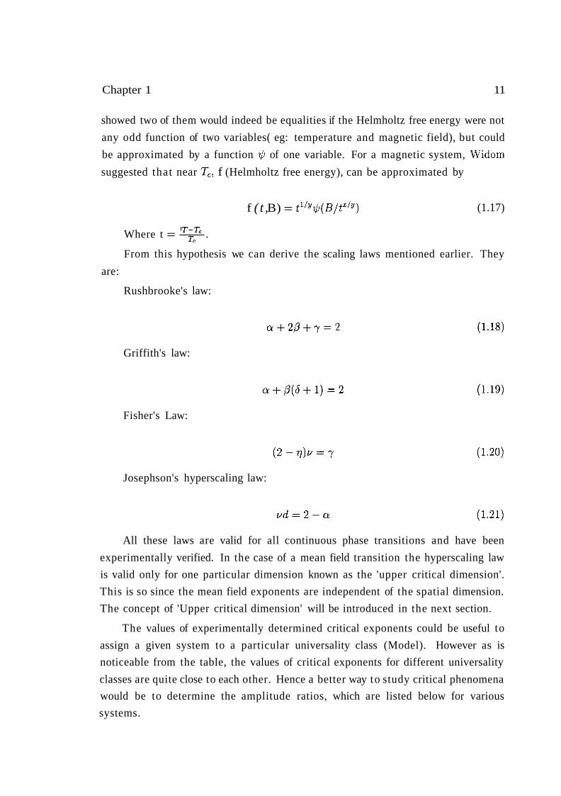
suggested that near T,, f (Helmholtz free energy), can be approximated by
f ( t , B) = t l l y$ (~ / tx ly ) (1.17)
JT-Tc 1 Where t = Tc .
From this hypothesis we can derive the scaling laws mentioned earlier. They
are:
Rushbrooke's law:
Griffith's law:
Fisher's Law:
Josephson's hyperscaling law:
All these laws are valid for all continuous phase transitions and have been
experimentally verified. In the case of a mean field transition the hyperscaling law
is valid only for one particular dimension known as the 'upper critical dimension'.
This is so since the mean field exponents are independent of the spatial dimension.
The concept of 'Upper critical dimension' will be introduced in the next section.
The values of experimentally determined critical exponents could be useful to
assign a given system to a particular universality class (Model). However as is
noticeable from the table, the values of critical exponents for different universality
classes are quite close to each other. Hence a better way to study critical phenomena
would be to determine the amplitude ratios, which are listed below for various
Mean field theories are valid for d > 4. This can be proved using a simple
criterion given by Ginzburg [3]. '
Basically the criterion says that mean field theories are valid if the square of
the fluctuations is much less than the square of the order parameter. As can be seen
intuitively , the effect of fluctuations is less in higher dimensions. This is because
each spin has more number of neighbours in higher dimensions and therefore the
energy required to cause a fluctuation is much greater in higher dimensions (crudely
speaking, more bonds have to be broken in higher dimensions). For d < 4 , the
Ginzburg criterion gives the range of temperature from T, beyond which mean field
theory is valid. The dimension above which mean field theory is valid is known as the
upper critical dimension. The upper critical dimension depends on the Hamiltonian
chosen to describe the system. For example if the Hamiltonian has only the M 6 and
h12 terms, the upper critical dimension is 3. Hence mean field theories are quite
suitable for a system described by such a Hamiltonian in 3 dimensions.
1 0.38
For d < d,, where d, is the upper critical dimension, mean field theory is valid
for temperatures sufficiently far from T,. As T approaches T, (either from above
or from below), fluctuations become more important and the inequality is violated.
The temperature TG at which fluctuations become important is called the Ginzburg
temperature and is given by
0.5 - 0.63 0.49 - 0.74
Where Ad is a constant for a fixed dimension d. to = is the bare
coherence length and AC, = % is the mean-field specific heat jump per unit
volume.
Thus? mean field theory will be valid even very close to a critical point for
4.5 - 5.0 5.0
2.0 1.7 - 2.0
Chapter 1 13
d < d,, if the bare coherence length J, is large. This is the case for systems with
long range forces. When ITG - T,I is not small, one can expect a crossover from T-T mean field behaviour to critical behaviour when the reduced temperature t =
becomes of order tG.
In 3-d, a careful evaluation of Ad yields [3]
1.4 Phase Transitions under High Pressure
In most of the discussion about phase transitions given above, temperature seems
to play the predominant role as far as the free energy of the system is concerned.
However the free energy of the system is also dependent on the pressure to which
the system is subjected to. The application of pressure changes the interatomic
interactions, leading to the appearance of new phases. In some cases, phases which
are not seen a t atmospheric pressures, make their appearance a t higher pressures.
There have been a few instances of re-entrant phase transitions a t high pressures.
This phenomenon has been observed in the case of metallic glasses and also in the
case of liquids [16] and liquid crystals.
Since ,the later chapters will deal with phase diagrams quite extensively, a gen-
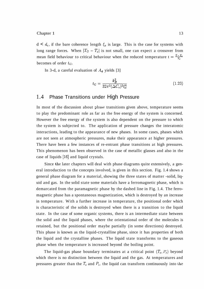
eral introduction to the concepts involved, is given in this section. Fig. 1.4 shows a
general phase diagram for a material, showing the three states of matter -solid, liq-
uid and gas. In the solid state some materials have a ferromagnetic phase, which is
demarcated from the paramagnetic phase by the dashed line in Fig. 1.4. The ferro-
magnetic phase has a spontaneous magnetization, which is destroyed by an increase
in temperature. With a further increase in temperature, the positional order which
is characteristic of the solids is destroyed when there is a transition to the liquid
state. In the case of some organic systems, there is an intermediate state between
the solid and the liquid phases, where the orientational order of the molecules is
retained, but the positional order maybe partially (in some directions) destroyed.
This phase is known as the liquid-crystalline phase, since it has properties of both
the liquid and the crystalline phases. The liquid state transforms to the gaseous
phase when the temperature is increased beyond the boiling point.
The liquid-gas phase boundary terminates a t a critical point (T,, PC) beyond
which there is no distinction between the liquid and the gas. At temperatures and
pressures greater than the Tc and PC, the liquid can transform continuously into the
Chapter 1
Figure 1.4: A typical Phase diagram showing the various possible phases
Chapter 1
Figure 1.5: Phase diagram for a ferromagnetic system showing the critical point
gaseous phase. This is possible as there is no symmetry difference between the liquid
and the gaseous phase. Both the solid-liquid transition and the liquid-gas transition
(except a t the critical point), are first order transitions.
The phase boundaries (in the case of first order transitions) are described by
the Clausius-Clayperon relation [2]:
A positive slope for the phase boundary means that both A S and A V are
positive o r b o t h of them are negative (which is more unlikely). A negative slope
usually implies that A V is negative . The only example for a negative AS is the
liquid-solid transition in Helium where the liquid phase is more ordered [2]. A V is
negative in the case of the melting transition in water.
The liquid-gas transition has many analogies with the ferromagnetic to para-
Chapter 1 16
magnetic transition. In the case of the ferro-para transition, the magnetization is
analogous to volume, while the magnetic field is analogous to the pressure. The
phase diagram for the ferro-para transition is shown in Fig. 1.5. The critical be-
haviour around this critical point fits the 3d Ising model.
In the case of a continuous phase transition, the R.H.S of Eq. 1.24 becomes
indeterminate as both A S and AV become zero for a continuous transition. In that
case the R.H.S of Eq. 1.24 is evaluated'using L'Hospital's rule. Differentiating the
numerator and the denominator of the indeterminate expression with respect to T, we have,
Where AC, is the discontin~li t~ in specific heat and A n , the discontinuity in
the coefficient of volume expansion. ,
Differentiating Eq. 1.24 with respect to P one obtains the other Ehrenfest re-
lation for a second-order transition [2]:
Where A,i3 is the discontinuity in compressibility a t the transition.
High pressure studies are also undertaken to investigate various multicritical
points [17] which occur in some systems.
1.5 Amorphous Magnetic systems
While critical phenomena in crystalline magnetic systems have been receiving quite
a bit of attention over a very long time, the critical behaviour of amorphous magnetic
systems has been studied only quite recently. The number of experimental studies
have been somewhat limited. The present study on amorphous magnetic systems
was motivated by a number of fundamental questions regarding the behaviour of
amorphous systems:
What is the nature of the critical behaviour in amorphous magnetic systems?
Is there a marked departure with respect to the corresponding crystalline systems?
Gubanov [18] showed that Ferromagnetism could exist in the amorphous state.
Harris [19] gave a physical estimate of the effect of fluctuations in T, due to the
presence of non-magnetic components in the sample as well as the fluctuations in
Ji, due to variations in the nearest neighbour distance.
The argument of Harris is as follows:
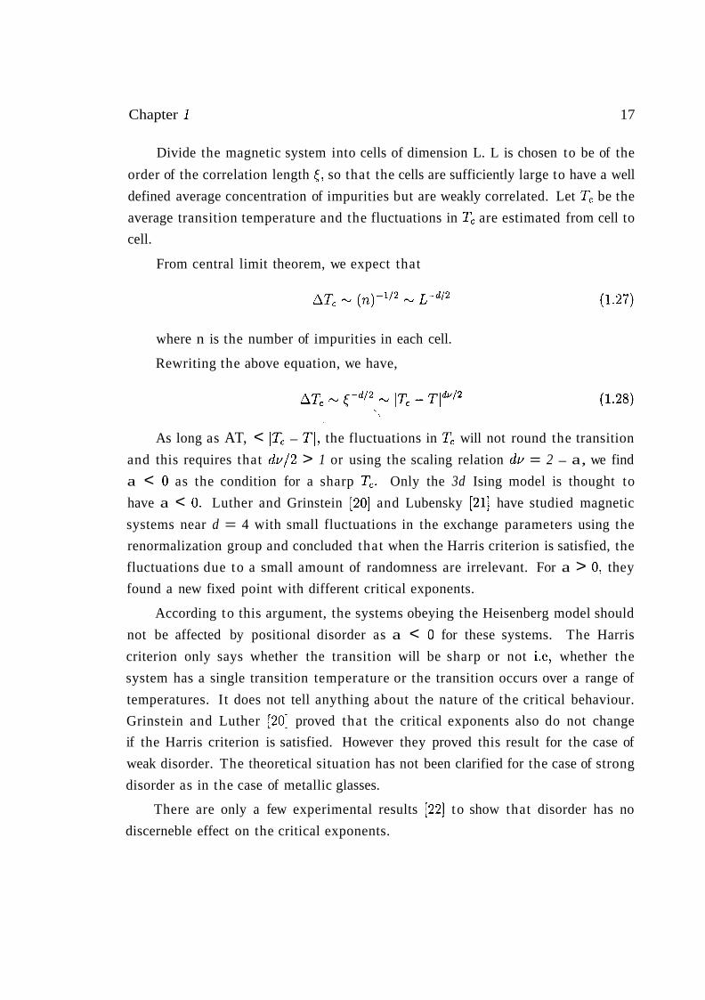
Chapter 1 17
Divide the magnetic system into cells of dimension L. L is chosen to be of the
order of the correlation length I, so that the cells are sufficiently large to have a well
defined average concentration of impurities but are weakly correlated. Let T, be the
average transition temperature and the fluctuations in T, are estimated from cell to
cell.
From central limit theorem, we expect that
where n is the number of impurities in each cell.
Rewriting the above equation, we have,
As long as AT, < IT, - TI, the fluctuations in T, will not round the transition
and this requires that d v / 2 > 1 or using the scaling relation d v = 2 - a, we find
a < 0 as the condition for a sharp T,. Only the 3d Ising model is thought to
have a < 0. Luther and Grinstein [20] and Lubensky [21] have studied magnetic
systems near d = 4 with small fluctuations in the exchange parameters using the
renormalization group and concluded that when the Harris criterion is satisfied, the
fluctuations due to a small amount of randomness are irrelevant. For a > 0 , they
found a new fixed point with different critical exponents.
According to this argument, the systems obeying the Heisenberg model should
not be affected by positional disorder as a < 0 for these systems. The Harris
criterion only says whether the transition will be sharp or not i.e, whether the
system has a single transition temperature or the transition occurs over a range of
temperatures. It does not tell anything about the nature of the critical behaviour.
Grinstein and Luther [20] proved that the critical exponents also do not change
if the Harris criterion is satisfied. However they proved this result for the case of
weak disorder. The theoretical situation has not been clarified for the case of strong
disorder as in the case of metallic glasses.
There are only a few experimental results [22] to show that disorder has no
discerneble effect on the critical exponents.
References
[I] H.E.Stanley, Introductioh to Phase transitions and Critical Phenomena, Oxford
University Press, 1971
[2] A.B.Pippard, Classical Thermodynamics, Cambridge University Press, 1963
[3] P.M. Chaikin and T.C. Lubensky, Principles of Condensed Matter Physics,
Cambridge University Press, 1995
[5] Wegner F.J., Phys.Rev.B., 5, 1889 (1972)
[6] E.Fawcett and W.A.,Reed, Phys.Rev.Lett., 9 , 336 (1962); E.Fawcett,
Adv.Phys., 13, 139 (1964); A.S.Joseph and A.C.Thorsen, Phys.Rev.Lett.,
L.Hodges,D.R.Stone and A.V.Gold, Phys.Rev.Lett., 19 , 655 (1967)
[7] N.D.Mermin and D.Wagner,Phys.Rev.Lett., 17, 1133 (1966)
[8] M.E.Fisher, Essays in Physics, vo1.4, Ed.G.K.T.Conn and G.N.Fowler, Aca-
demic Press, 1972
[lo] C.Kitte1, Introduction to Solid State Physics, Wiley Eastern Pvt. ltd., New
Delhi, 1971
[ll] Rushbrooke, J.ChemiPhys., 39, 842 (1963)
Chapter 1
[15] B.Widom, J.Chem.Phys., 43, 3892 (1965)
[16] Anil Kumar and T.Narayanan, Phys.Rep. ,249, 135 (1994)
[17] Anil Kumar, H.R.Krishnamurthy and E.S.R.Gopa1, Phys.Rep., 98, 57 (1983)
[18] A.I.Gubanov in Quantum Electron Theory of Amorphous Conductors, Consul-
tants Bureau, New York, 1965
[19] A.B. Harris, J.Phys.C7, 1671 (1974)
[20] A.Grinstein and A.Luther, Phys.Rev.B 13, 1329 (1976)
[21] T.C.Lubensky in Ill-Condensed Matter, Proceedings of Les Houches school,
Edited by Roger Balian, Roger Maynard and Gerard Toulouse, 1978
[22] L.J. Schowalter, M.B. Salamon, C.C.Tsuei and R.A. Craven, Sol.State.Comm,
24, 525 (1977)
Chapter 2
High Pressure Instrumentation
2.1 Introduction
The Piston-cylinder apparatus is a well known device in the field of high pressure
research. The piston-cylinder device use'd in the present work can attain pressures
of the order of 50 kbars. The maximum pressure which can be attained is set by the
strength of the tungsten carbide plates which are used to contain the sample. While
higher pressures are obtained in the Diamond anvil technique, the piston-cylinder
technique has the advantages of a large sample size and a true hydrostatic pressure.
The piston-cylinder apparatus is discussed in detail in this chapter. The cell-
assemblies used in the present experimental work, as well as the techniques used for
the measurement of resistivity and thermopower are also described.
2.2 Piston-Cylinder Apparatus
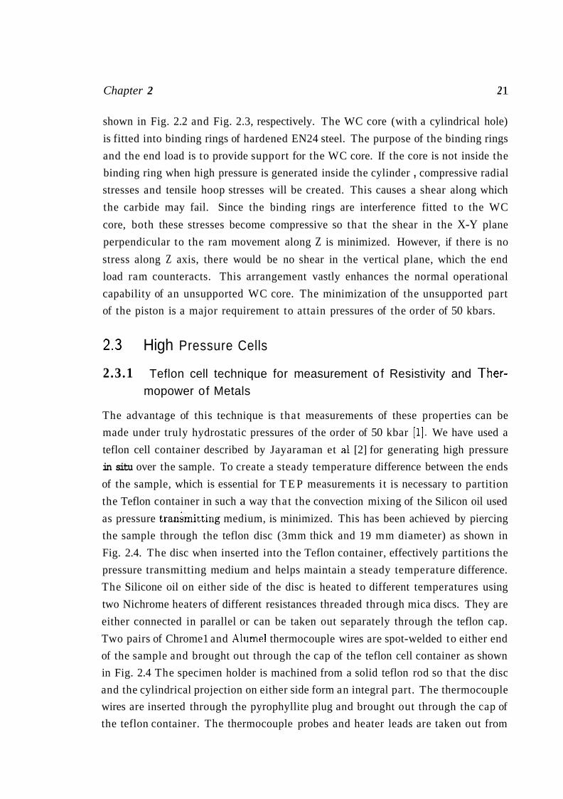
The high pressure apparatus used in the present investigation is a piston-cylinder
device and very high pressures can be generated by the advance of a one inch or
half inch diameter piston into a cylinder, both made of tungsten carbide (WC). The
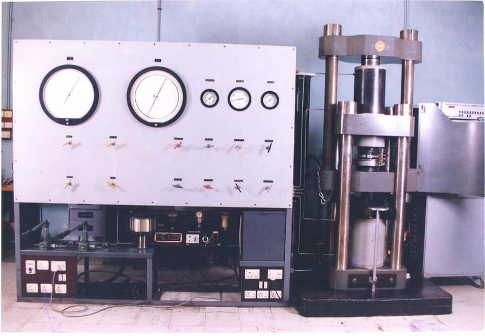
entire arrangement (Fig. 2.1) consists of a ten inch diameter master ram of 1000
ton capacity. The entire arrangment of the pistion-cylinder apparatus together with
the pressure controls is shown in the photograph appearing in the next page. The
piston assembly is advanced by operating this master ram. Since WC is strong
in compression and weak in tension or shear, precautions have to be taken to see
that it is always under compressive load. When high pressure is generated in the
cylindrical WC core there will be a tensile lateral force acting along the asis of the
cylinder. To compensate for this, the cylinder is supported axially by an end load
ram of 750 ton capacity. The pressure plate assembly and the end load plate are
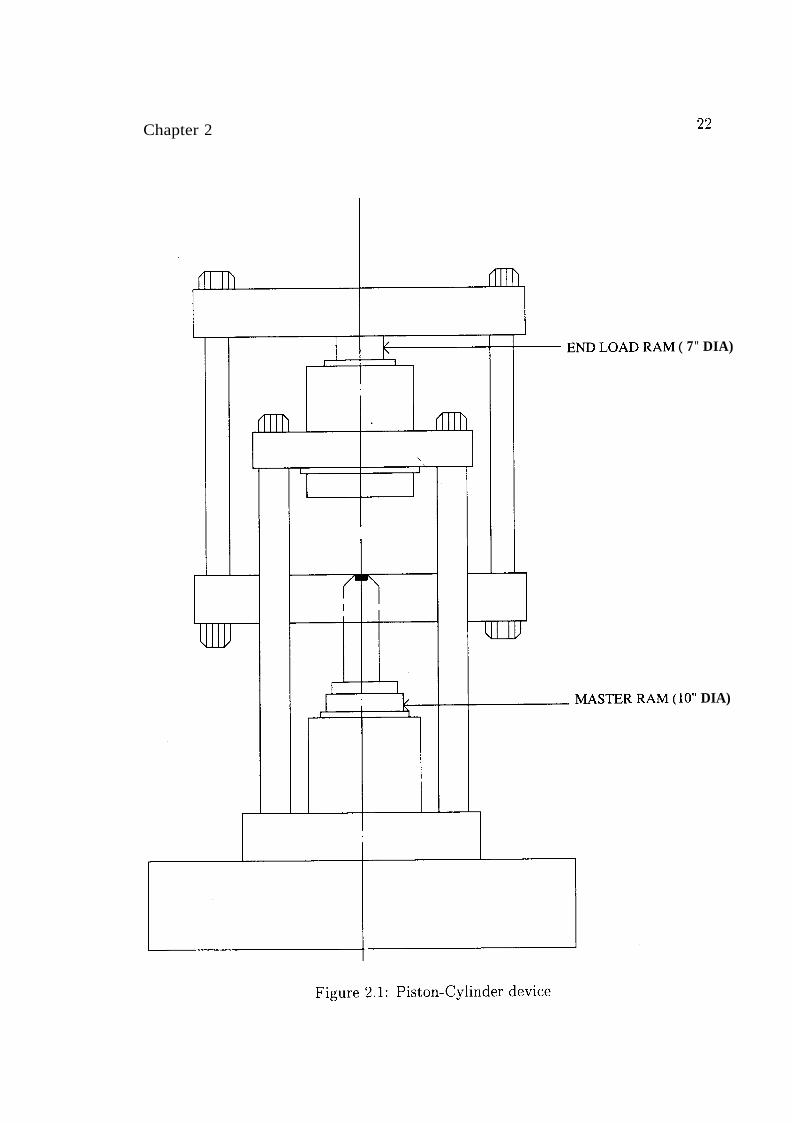
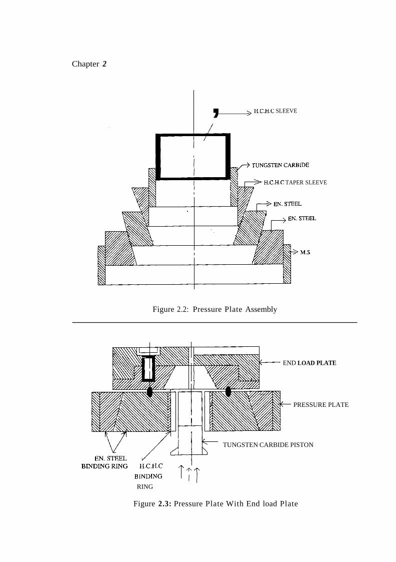
Chapter 2 2 1
shown in Fig. 2.2 and Fig. 2.3, respectively. The WC core (with a cylindrical hole)
is fitted into binding rings of hardened EN24 steel. The purpose of the binding rings
and the end load is to provide support for the WC core. If the core is not inside the
binding ring when high pressure is generated inside the cylinder , compressive radial
stresses and tensile hoop stresses will be created. This causes a shear along which
the carbide may fail. Since the binding rings are interference fitted to the WC
core, both these stresses become compressive so that the shear in the X-Y plane
perpendicular to the ram movement along Z is minimized. However, if there is no
stress along Z axis, there would be no shear in the vertical plane, which the end
load ram counteracts. This arrangement vastly enhances the normal operational
capability of an unsupported WC core. The minimization of the unsupported part
of the piston is a major requirement to attain pressures of the order of 50 kbars.
High Pressure Cells
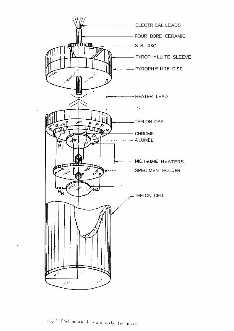
2.3.1 Teflon cell technique for measurement of Resistivity and Ther- mopower of Metals
The advantage of this technique is that measurements of these properties can be
made under truly hydrostatic pressures of the order of 50 kbar [I]. We have used a
teflon cell container described by Jayaraman et a1 [2] for generating high pressure
in situ over the sample. To create a steady temperature difference between the ends
of the sample, which is essential for T E P measurements it is necessary to partition
the Teflon container in such a way that the convection mixing of the Silicon oil used
as pressure transmitting medium, is minimized. This has been achieved by piercing
the sample through the teflon disc (3mm thick and 19 mm diameter) as shown in
Fig. 2.4. The disc when inserted into the Teflon container, effectively partitions the
pressure transmitting medium and helps maintain a steady temperature difference.
The Silicone oil on either side of the disc is heated to different temperatures using
two Nichrome heaters of different resistances threaded through mica discs. They are
either connected in parallel or can be taken out separately through the teflon cap.
Two pairs of Chrome1 and Alumel thermocouple wires are spot-welded to either end
of the sample and brought out through the cap of the teflon cell container as shown
in Fig. 2.4 The specimen holder is machined from a solid teflon rod so that the disc
and the cylindrical projection on either side form an integral part. The thermocouple
wires are inserted through the pyrophyllite plug and brought out through the cap of
the teflon container. The thermocouple probes and heater leads are taken out from
Chapter 2
( 7" DIA)
:lo" DIA)
Chapter 2
I , > H.C.H.C SLEEVE
--) H.C.H.C TAPER SLEEVE
Figure 2.2: Pressure Plate Assembly
END LOAD PLATE
PRESSURE PLATE
TUNGSTEN CARBIDE PISTON
RING
Figure 2.3: Pressure Plate With End load Plate
ELECTRICAL LE
FOUR BORE CE
S.S. DlSC
. PYROPHY LLI TE
PYROPH YLLITE
-TEFLON CAP
CHROMEL ALUMEL
NICHROME HEA
SPECIMEN HOL
TEFLON CELL
ADS
RAMIC
SLEEVE
DlSC
-HEATER LEAD
TERS.
D ER
Chapter 2 2 4
the high pressure region to the atmospheric pressure region in a manner described
by Jayaraman et a1 [2]. The thermocouple leads are taken out through four hole
ceramic tubings and connected to the appropriate wires coming out of the cap of
the teflon cell by spot-welding the junction. By this the generation of thermo-
electric noise voltages due to temperature fluctuations is completely avoided as no
new metal is used for bonding. The pyrophyllite disc and the stainless steel piece
with a pyrophyllite ring assembly, through which the ceramic tubing is inserted
helps in holding the ceramic tube in position under pressure. At low pressures the
stainless steel disc flows and grips the ceramic whereas a t high pressures the lower
pyrophyllite disc provides the necessary grip for the ceramic. One of the heater
leads which passes through the hole in the pyrophyllite disc makes contact with
the stainless steel piece which in turn will be touching the end load plate of the
pressure chamber. The other heater wire touches the pressure plate directly. The
pressure plate and the end load plate which are insulated from each other acts as
the terminals for current to be passed. The teflon cell assembly is positioned inside
the pressure chamber. The pressure chamber made out of the WC core fitted with
steel binding rings described earlier is the one used in the piston-cylinder device.
In any pressure experiment, there will always be a small length of the wire that
suffers a large pressure gradient while it is brought from the high pressure to the
atmospheric pressure region. This small region is inhomogeneous in its properties
and for T E P measurements it is essential that in these portions of the wire there are
no temperature gradients. The cell we are using almost satisfies this requirement be-
cause of the internal heating arrangement and smaller diameter of wires used which
reduces thermal conduction through the wires. The cell provides a temperature
gradient varying from 0.25" C to 1 5 O C in the temperature range 0-250" C.
The same cell can also be used for 4-probe resistivity measurement. The only
modification required would be to see that no temperature gradient exists across
the sample. This is achieved by positioning the sample horizontally in the cell and
removing the partitioning disc.
The teflon cell has been used for measuring the resistivity and thermopower of
Chromium alloys. These are dealt with in chapter 6.
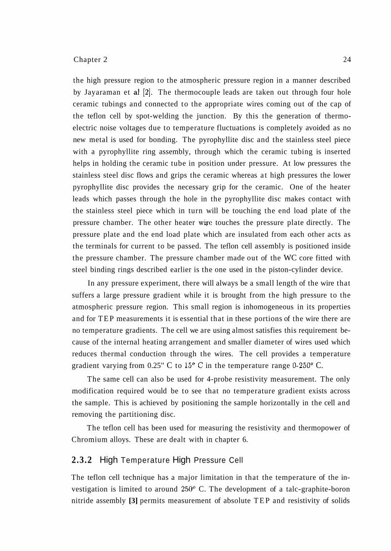
2.3.2 High Temperature High Pressure Cell
The teflon cell technique has a major limitation in that the temperature of the in-
vestigation is limited to around 250' C. The development of a talc-graphite-boron
nitride assembly [3] permits measurement of absolute T E P and resistivity of solids
+- THE RMOCOUPLE LEADS
Chapter 2 26
and liquids in the temperature range 0 - 1000" C and 50 kbar pressure. The tem-
perature profile in a graphite heater will in general have a non-uniform temperature
zone near the ends and a constant temperature zone in the region away from the
ends of the heater. The constant temperature zone is normally located-in the vicin-
ity of the geometric center of the furnace and is usually of one quarter of the length
in its spread. Since for the measurement of T E P the specimen has to be subjected
to a temperature gradient, the natural temperature profile of the furnace can be
exploited by proper positioning of the specimen in the furnace.
Talc and pyrophyllite are good solid pressure transmitters and can also stand
high temperatures which has made them suitable for our use. These materials,
unlike the fluid (Silicone oil) used in the teflon cell technique, cannot produce a
truly hydrostatic pressure over the sample. Although the distribution of pressure is
not uniform over a wide region, by using small samples (0.5 x 0.5 x 0.2 mm3) it is
possible to subject it to nearly hydrostatic pressure conditions.
The thermocouple leads are either spot-welded or embedded in to the specimen
and are taken out through the side holes in the sleeve along the grooves made on its
surface which are 90" apart. The sleeve-specimen assembly is inserted into a Boron
Nitride cup and the four leads were threaded through the boron nitride cap. These
four leads are brought out from the high pressure to the atmospheric pressure region
in a way similar to that in teflon cell technique. As boron nitride which is a good
thermal conductor is used to contain the sample, the temperature gradients in the
regions where the leads suffer a large pressure gradient is minimized.
The graphite heater is powered from a high current (500 Amps) low voltage (10
V) transformer. The current through the heater can be increased gradually by a
continuous scan of the voltage on the primary side of the transformer with the help
of a motor-gear arrangement coupled to the transformer. This facility allows one to
select a convenient heating rate.
The cell for resistivity measurement is the same as above except for the posi-
tioning of the sample. For resistivity measurements the important requirement is
that the temperature gradient across the sample length should be minimized. This
is achieved by keeping the sample horizontaIly inside the boron nitride container
which is a good thermal conductor and also by placing the sample in the constant
temperature zone of the graphite furnace. The effects of non-hydrostatic pressure
distribution can be further minimized if the distance between the two voltage leads
in the four probe method of measuring the resistivity is made smaller. Then one
would be measuring that part of the resistance between these two voltage leads
Chapter 2
10 20 30 40 50 60 70 80 Ram Pressure (Bars)
Figure 2.6: Resistance versus Pressure for Bismuth in a 112" Teflon cell
which is subjected to nearly hydrostatic pressure conditions, although the rest of
the sample is in the non uniform pressure region.
2.3.3 Pressure Calibration
There has been an extensive survey on the problem of high pressure calibration in
different pressure and temperature ranges [4]. This problem will not be dwelt with
in detail except to give the pressure calibration procedures which were carried out
for the present system [ 5 ] , using the high pressure cells described in the previous
sections.
The pressure calibration a t room temperature was done by the standard fixed
point method resulting from polymorphic phase transitions in some well known
metals. In the pressure range 0-40 kbar, the Bismuth 1-11 and 11-111 transitions were
utilized to calibrate the ram pressure against the true pressure seen by the specimen
in different cells. Electrical resistance measurements were done to monitor these
phase transitions. Fig. 2.6 and Fig. 2.7 give the relative resistance versus pressure
graph for high purity (99.99%) bismuth a t 25' C in the 112" teflon cell and 1/2"
high temperature high pressure cell. Similar runs were carried out in the 1" teflon
and 1" high temperature high pressure cells. Table. 2.1 summarizes the pressure
Chapter 2
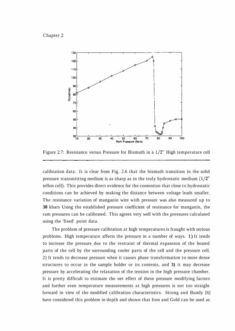
Figure 2.7: Resistance versus Pressure for Bismuth in a 112" High temperature cell
calibration data. I t is clear from Fig. 2.6 that the bismuth transition in the solid
pressure transmitting medium is as sharp as in the truly hydrostatic medium (112"
teflon cell). This provides direct evidence for the contention that close to hydrostatic
conditions can be achieved by making the distance between voltage leads smaller.
The resistance variation of manganin wire with pressure was also measured up to
30 kbars Using the established pressure coefficient of resistance for manganin, the
ram pressures can be calibrated. This agrees very well with the pressures calculated
using the 'fixed' point data.
The problem of pressure calibration a t high temperatures is fraught with serious
problems. High temperature affects the pressure in a number of ways. 1) It tends
to increase the pressure due to the restraint of thermal expansion of the heated
parts of the cell by the surrounding cooler parts of the cell and the pressure cell.
2) It tends to decrease pressure when it causes phase transformation to more dense
structures to occur in the sample holder or its contents, and 3) i t may decrease
pressure by accelerating the relaxation of the tension in the high pressure chamber.
It is pretty difficult to estimate the net effect of these pressure modifying factors
and further even temperature measurements a t high pressures is not too straight
forward in view of the modified calibration characteristics. Strong and Bundy [6]
have considered this problem in depth and shown that Iron and Gold can be used as
Chapter 2 30
pressure calibrants a t high temperatures. The a - y (BCC --+ FCC) phase boundary
in Iron has a good pressure sensitivity of about -4" C/kbar in the pressure region
20-60 kbar. Further this transformation can be easily monitored by either electrical
resistance or T E P measurements. Since the a - y boundary has been accurately
established due to the painstaking efforts of several workers in this field, pressure
calibration up to 800" C can be easily carried out. Table. 2.2 summarizes .the
calibration data for our high pressure , obtained through a number of experiments
on the a - y transition in Iron using both resistivity and TEP as tools. Chromel-
Alumel thermocouple which has a small pressure calibration error [7] was used for
temperature measurement in this work.
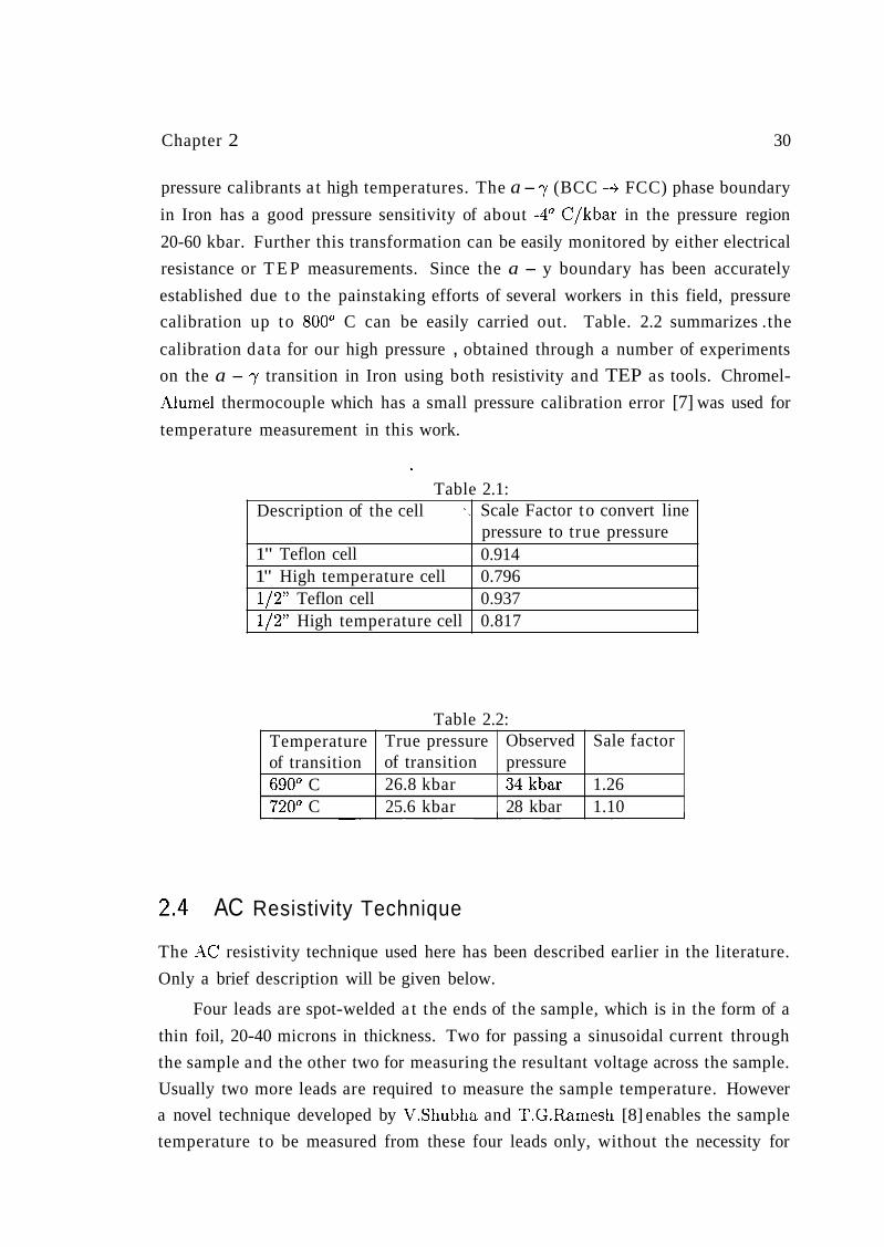
Table 2.1: Description of the cell ,i
1" Teflon cell 1" High temperature cell 112" Teflon cell 112" High temperature cell
AC Resistivity Technique
Scale Factor to convert line pressure to true pressure 0.914 0.796 0.937 0.817
Table 2.2:
The .4C resistivity technique used here has been described earlier in the literature.
Only a brief description will be given below.
Four leads are spot-welded a t the ends of the sample, which is in the form of a
thin foil, 20-40 microns in thickness. Two for passing a sinusoidal current through
the sample and the other two for measuring the resultant voltage across the sample.
Usually two more leads are required to measure the sample temperature. However
a novel technique developed by V.Shubha and T.G.Ramesh [8] enables the sample
temperature to be measured from these four leads only, without the necessity for
Sale factor
1.26 1.10
Temperature of transition 690" C 720" C
True pressure of transition 26.8 kbar 25.6 kbar
Observed pressure 34kbar 28 kbar
lOHa to lf Hz Ob(10mA
L Current Source
t f
Quadrature 08cill~t0r -
,
Pilbr
Sinwt
-
a Awtager
!
pamalcm.
Power Amp
I
a . . Chroma1 -- '- - 1
. I L t l m m l U I n
Flgore 2.8: Block Diagram of the AC R.rlrtlrlty wtup i
PC BASED
D M
Alumel
I
. . a
-v
- Chrome1
Alumel .
Ref LOCK-IN
Amplitier Conrt* .
-
Chapter 2 32
two extra leads. The standard technique which requires six leads to be taken out
from the high pressure cell of diameter less than 12 mm is quite difficult.
The two wires attached a t each end of the sample are actually Chromel-Alumel
thermocouple wires. The AC current is passed through Chrome1 wires, while the
voltage across the sample is measured using the Alumel wires.
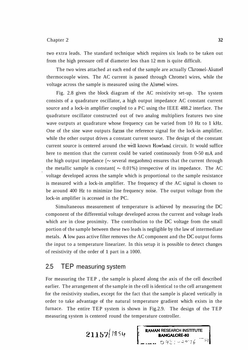
Fig. 2.8 gives the block diagram of the AC resistivity set-up. The system
consists of a quadrature oscillator, a high output impedance AC constant current
source and a lock-in amplifier coupled to a P C using the IEEE 488.2 interface. The
quadrature oscillator constructed out of two analog multipliers features two sine
wave outputs a t quadrature whose frequency can be varied from 10 Hz to 1 kHz.
One of the sine wave outputs forms the reference signal for the lock-in amplifier.
while the other output drives a constant current source. The design of the constant
current source is centered around the wk.11 known Howland circuit. I t would suffice
here to mention that the current could be varied continuously from 0-50 mA and
the high output impedance ( N several megaohms) ensures that the current through
the metallic sample is constant( - 0.01%) irrespective of its impedance. The AC ' voltage developed across the sample which is proportional to the sample resistance
is measured with a lock-in amplifier. The frequency of the AC signal is chosen to
be around 400 Hz to minimize line frequency noise. The output voltage from the
lock-in amplifier is accessed in the PC.
Simultaneous measurement of temperature is achieved by measuring the DC
component of the differential voltage developed across the current and voltage leads
which are in close proximity. The contribution to the DC voltage from the small
portion of the sample between these two leads is negligible by the law of intermediate
metals. A low pass active filter removes the AC component and the DC output forms
the input to a temperature linearizer. In this setup it is possible to detect changes
of resistivity of the order of 1 part in a 1000.
2.5 TEP measuring system
For measuring the T E P , the sample is placed along the axis of the cell described
earlier. The arrangement of the sample in the cell is identical to the cell arrangement
for the resistivity studies, except for the fact that the sample is placed vertically in
order to take advantage of the natural temperature gradient which exists in the
furnace. The entire T E P system is shown in Fig.2.9. The design of the T E P
measuring system is centered round the temperature controller.
--- RAMAN RESEARCH INSTITUTE
BANGALORE-80 3 9; ; r q * -j&
--- J J O '
Ir 1 - a. I
Simulator
Simulator IzTI Flgan 4.9: TEP moa8trrlng ny#km
Chapter 2 33
The temperature control is implemented using a PID algorithm integrated into
the software. The D/A (16 bit) of a DSP lock-in amplifier (SRS 830) was used for
this purpose. The output of the D/A is fed to the power amplifier which supplies
the requisite power to the heater.
An important requisite for T E P measurement is the control of the temperature
gradient. The control of the temperature gradient is such that, while the mean
temperature T is held constant, the magnitude of the temperature difference AT across the ends of the sample can be altered a t will.
To calculate the thermo-emf ,S, of the sample, the voltages VchT-sam-chT and
VAlu-sam-Alu were measured using a Keithley digital multimeter (DMM). The DMICI
(model 2001) was interfaced to a personal computer using IEEE 488.2 interface card.
The programmes for the interfacing were written in the VIEWDAC environment
supplied by Keithley. The VIEWDAC environment allows for real-time plotting of
the data.
The absolute TEP, S , of the sample , in the differential mode of measurement
,is given by [9],
Where Schr and Schr-alu are the absolute thermopower of Chromel and the
thermopower of the Chromel-Alumel thermocouples respectively. VchT-sam-chr and
Valu-sam-alu are the differential voltages developed across the thermocouples formed
out of the reference probes and the specimen, when a small temperature difference
is maintained across the length of the sample. In order t o evaluate S as a function
of temperature, it is necessary to simulate the temperature dependence of both SchT
and Schr-alu.
Since T E P in the differential mode of measurement is related to the limiting
value of the quantity in the square bracket in the expression for S as A T -+ 0, the
system should have the provision to evaluate this quantity for different A T holding
the mean temperature T constant. These requirements have been met by employing
two separate controllers for the variables T and AT.
The non-linear variations with temperature of the physical quantities like the
absolute T E P of Chromel (Schr) and the relative T E P of Chromel-Alumel thermo-
couple (SchT-alu) are simulated by employing a sixth-order polynomial curve fit
Chapter 2
Where b,.. . .b6 and c,. . .. .c6 are constants. These constants can be evaluated from
computer fit of the NBS data [lo].
An algorithm based on the above expressions forms the basis for simulating SchT
and Schr-alu-
In order to obtain a higher precision in the fit, the temperature range was
divided into two blocks namely 0"-200" C and 200" - 1000" C. The fitting error for
SchT-alu in the two ranges are &O.O04"pV/" C and *O.O3pV/O C.
For Schr the fitting errors are f O.OO1pVIO C and &O.lpV/" C on the two ranges.
The overall accuracy of TEP measurement is - 0.5% and the resolution is