Chapter 1 GRASP FOR LINEAR INTEGER PROGRAMMING Teresa Neto [email protected]Jo˜ ao Pedro Pedroso [email protected]Departamento de Ciˆ encia de Computadores Faculdade de Ciˆ encias da Universidade do Porto Rua do Campo Alegre, 823 4150-180 Porto, Portugal Abstract In this paper we introduce a GRASP for the solution of general linear integer problems. The strategy is based on the separation of the set of variables into the integer subset and the continuous subset. The integer variables are fixed by GRASP and replaced in the original linear prob- lem. If the original problem had continuous variables, it becomes a pure continuous problem, which can be solved by a linear program solver to determine the objective value corresponding to the fixed variables. If the original problem was a pure integer problem, simple algebraic manipu- lations can be used to determine the objective value that corresponds to the fixed variables. When we assign values to integer variables that lead to an impossible linear problem, the evaluation of the corresponding so- lution is given by the sum of infeasibilities, together with an infeasibility flag. We report results obtained for some standard benchmark problems, and compare them to those obtained by branch-and-bound and to those obtained by an evolutionary solver. Keywords: GRASP, Linear Integer Programming 1. Introduction A wide variety of practical problems can be solved using integer lin- ear programming. Typical problems of this type include lot sizing, scheduling, facility location, vehicle routing, and more; see for exam- ple (Nemhauser and Wolsey 1988, Wolsey 1998).
Departamento de Ciencia de ComputadoresFaculdade de Ciencias da Universidade do PortoRua do Campo Alegre, 8234150-180 Porto, Portugal
Abstract In this paper we introduce a GRASP for the solution of general linearinteger problems. The strategy is based on the separation of the set ofvariables into the integer subset and the continuous subset. The integervariables are fixed by GRASP and replaced in the original linear prob-lem. If the original problem had continuous variables, it becomes a purecontinuous problem, which can be solved by a linear program solver todetermine the objective value corresponding to the fixed variables. If theoriginal problem was a pure integer problem, simple algebraic manipu-lations can be used to determine the objective value that corresponds tothe fixed variables. When we assign values to integer variables that leadto an impossible linear problem, the evaluation of the corresponding so-lution is given by the sum of infeasibilities, together with an infeasibilityflag.
We report results obtained for some standard benchmark problems,and compare them to those obtained by branch-and-bound and to thoseobtained by an evolutionary solver.
Keywords: GRASP, Linear Integer Programming
1. IntroductionA wide variety of practical problems can be solved using integer lin-
ear programming. Typical problems of this type include lot sizing,scheduling, facility location, vehicle routing, and more; see for exam-ple (Nemhauser and Wolsey 1988, Wolsey 1998).
2
In this paper we introduce a GRASP (greedy randomized adaptivesearch procedure) for the solution of general linear integer programs.The strategy is based on the separation of the set of variables into theinteger subset and the continuous subset (if some). The procedure startsby solving the linear programming (LP) relaxation of the problem. Val-ues for the integer variables are then chosen, through a semi-greedyconstruction heuristic based on rounding around the LP relaxation, andfixed. The continuous variables (if some) can then be determined in func-tion of them, by solving a linear program where all the integer variableshave been fixed by GRASP. Afterwards, local search improvements aremade on this solution; these improvements still correspond to changesmade exclusively on integer variables, after which the continuous vari-ables are recomputed through the solution of an LP. When the linearprogram leads to a feasible solution, the evaluation of the choice of thevariables is determined directly by the objective function. If the choiceof the variables induces an infeasible problem, its evaluation is measuredby the sum of infeasibilities.
2. BackgroundIn this paper we focus on the problem of optimizing a linear function
subject to a set of linear constraints, in the presence of integer and,possibly, continuous variables. The more general case, where there areinteger and continuous variables, is usually called mixed integer (MIP).
The general formulation of a mixed integer linear program is
maxx,y
{cx + hy : Ax + Gy ≤ b, x ∈ Zn+, y ∈ Rp
+}, (1.1)
where Zn+ is the set of nonnegative, n-dimensional integral vectors, and
Rp+ is the set of nonnegative, p-dimensional real vectors. A and G are m×
n and m×p matrices, respectively, where m is the number of constraints.There are n integer variables (x), and p continuous variables (y).
If the subset of continuous variables is empty, the problem is calledpure integer (IP); its formulation is
maxx{cx : Ax ≤ b, x ∈ Zn
+}. (1.2)
In general, there are additional bound restrictions on the integer vari-ables, stating that li ≤ xi ≤ ui, for i = 1, . . . , n.
The main idea for the conception of the algorithm described in thispaper is provided in (Pedroso 1998; 2002). It consists of fixing the in-teger variables of a linear integer program by a meta-heuristic—in thiscase GRASP. For MIP, by replacing these variables on the original for-mulation, we obtain a pure, continuous LP, whose solution provides anevaluation of the fixed variables. On the case of pure IP, we can com-pute directly the corresponding objective. We can also directly checkfeasibility, and compute the constraints’ violation.
GRASP for linear integer programming 3
Notice that this algorithm, as opposed to branch-and-bound, does notwork with the solution of continuous relaxations of the initial problem.The solution of LPs is only required for determining the value of the con-tinuous variables, and of the objective that corresponds to a particularinstantiation of the integer variables.
Instances of integer linear problems correspond to specifications ofthe data: the matrix A and the vectors b and c in Equations 1.1 and 1.2for IPs, and also the matrix G and the vector h for MIPs. The mostcommonly used representation of instances of these problems is throughMPS files, which is the format used on this GRASP implementation.We have tested GRASP with a subset of the benchmark problems thatare available in this format in the MIPLIB (Bixby et al. 1998).
3. GRASPGRASP (Feo and Resende 1989; 1995, Pitsoulis and Resende 2002,
Resende and Ribeiro 2001) is a meta-heuristic based on a multi-startprocedure where each iteration has two phases: construction and localsearch. In the construction phase, a solution is built, one element at atime. At each step of this phase, the candidate elements that can beincorporated to the partial solution are ranked according to a greedyfunction. The evaluation of these elements leads to the creation of arestricted candidate list (RCL), where a selection of good variables, ac-cording to the corresponding value of the greedy function, are inserted.At each step, one element of the RCL is randomly selected and incor-porated into the partial solution (this is the probabilistic component ofthe heuristic). The candidate list and the advantages associated withevery element are updated (adaptive component of the heuristic). Thenumber of elements of the RCL is very important for GRASP: if theRCL is restricted to a single element, then only one, purely greedy solu-tion will be produced; if the size of the RCL is not restricted, GRASPproduces random solutions. The mean and the variance of the objectivevalue of the solutions built are directly affected by the cardinality of theRCL: if the RCL has more elements, then more different solutions willbe produced, implying a larger variance.
The solutions generated in the construction phase generally are notlocal optima, with respect to some neighborhood. Hence, they can oftenbe improved by means of a local search procedure. The local search phasestarts with the constructed solution and applies iterative improvementsuntil a locally optimal solution is found.
The construction and improvement phases are repeated a specifiednumber of times. The best solution over all these GRASP iterations isreturned as the result.
In Algorithm 1 we present the structure of a general GRASP algo-rithm.
4
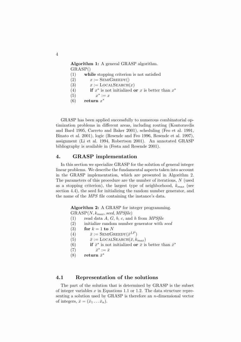
Algorithm 1: A general GRASP algorithm.GRASP()(1) while stopping criterion is not satisfied(2) x := SemiGreedy()(3) x := LocalSearch(x)(4) if x∗ is not initialized or x is better than x∗
(5) x∗ := x(6) return x∗
GRASP has been applied successfully to numerous combinatorial op-timization problems in different areas, including routing (Kontoravdisand Bard 1995, Carreto and Baker 2001), scheduling (Feo et al. 1991,Binato et al. 2001), logic (Resende and Feo 1996, Resende et al. 1997),assignment (Li et al. 1994, Robertson 2001). An annotated GRASPbibliography is available in (Festa and Resende 2001).
4. GRASP implementationIn this section we specialize GRASP for the solution of general integer
linear problems. We describe the fundamental aspects taken into accountin the GRASP implementation, which are presented in Algorithm 2.The parameters of this procedure are the number of iterations, N (usedas a stopping criterion), the largest type of neighborhood, kmax (seesection 4.4), the seed for initializing the random number generator, andthe name of the MPS file containing the instance’s data.
Algorithm 2: A GRASP for integer programming.GRASP(N, kmax, seed,MPSfile)(1) read data A, G, b, c, and h from MPSfile(2) initialize random number generator with seed(3) for k = 1 to N(4) x := SemiGreedy(xLP )(5) x := LocalSearch(x, kmax)(6) if x∗ is not initialized or x is better than x∗
(7) x∗ := x(8) return x∗
4.1 Representation of the solutionsThe part of the solution that is determined by GRASP is the subset
of integer variables x in Equations 1.1 or 1.2. The data structure repre-senting a solution used by GRASP is therefore an n-dimensional vectorof integers, x = (x1 . . . xn).
GRASP for linear integer programming 5
4.2 Evaluation of solutionsThe solutions on which the algorithm works may be feasible or not.
For the algorithm to function appropriately it has to be able to dealwith both feasible and infeasible solutions in the same framework. Wedescribe next the strategies used for tackling this issue on MIPs and IPs.
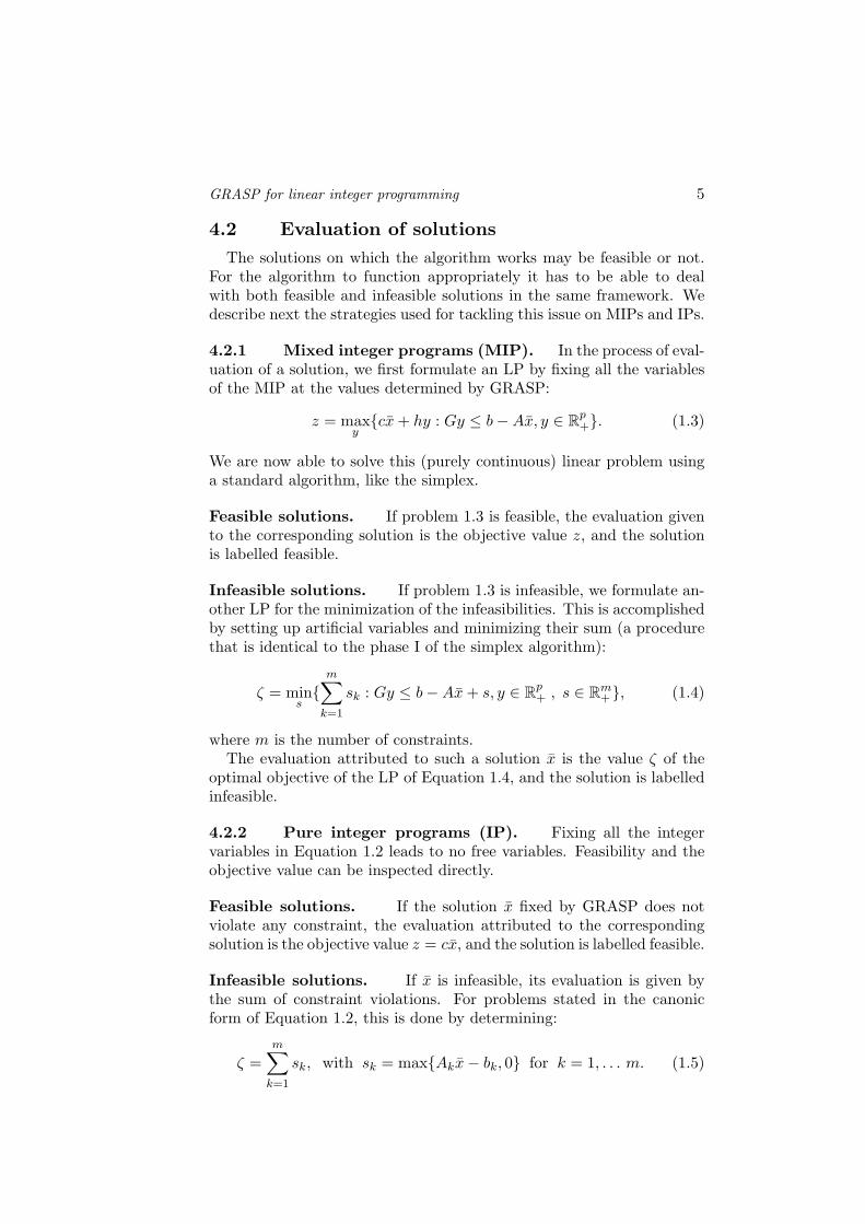
4.2.1 Mixed integer programs (MIP). In the process of eval-uation of a solution, we first formulate an LP by fixing all the variablesof the MIP at the values determined by GRASP:
z = maxy{cx + hy : Gy ≤ b−Ax, y ∈ Rp
+}. (1.3)
We are now able to solve this (purely continuous) linear problem usinga standard algorithm, like the simplex.
Feasible solutions. If problem 1.3 is feasible, the evaluation givento the corresponding solution is the objective value z, and the solutionis labelled feasible.
Infeasible solutions. If problem 1.3 is infeasible, we formulate an-other LP for the minimization of the infeasibilities. This is accomplishedby setting up artificial variables and minimizing their sum (a procedurethat is identical to the phase I of the simplex algorithm):
ζ = mins{
m∑k=1
sk : Gy ≤ b−Ax + s, y ∈ Rp+ , s ∈ Rm
+}, (1.4)
where m is the number of constraints.The evaluation attributed to such a solution x is the value ζ of the
optimal objective of the LP of Equation 1.4, and the solution is labelledinfeasible.
4.2.2 Pure integer programs (IP). Fixing all the integervariables in Equation 1.2 leads to no free variables. Feasibility and theobjective value can be inspected directly.
Feasible solutions. If the solution x fixed by GRASP does notviolate any constraint, the evaluation attributed to the correspondingsolution is the objective value z = cx, and the solution is labelled feasible.
Infeasible solutions. If x is infeasible, its evaluation is given bythe sum of constraint violations. For problems stated in the canonicform of Equation 1.2, this is done by determining:
ζ =m∑
k=1
sk, with sk = max{Akx− bk, 0} for k = 1, . . . m. (1.5)
6
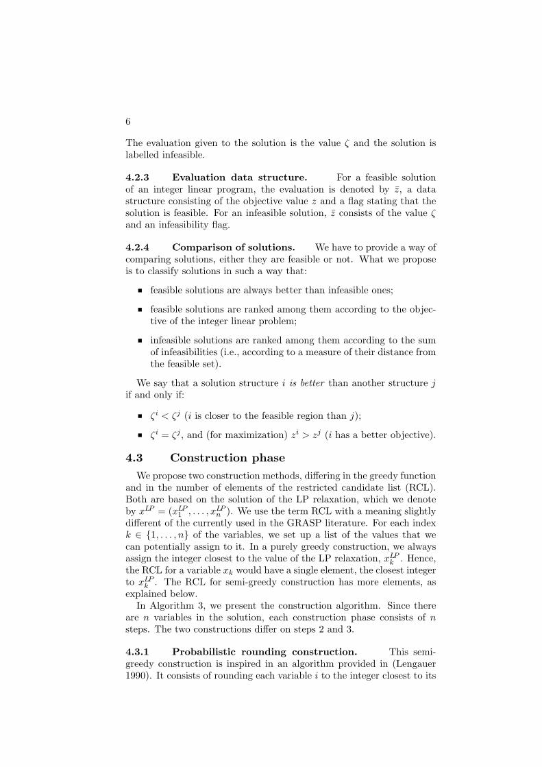
The evaluation given to the solution is the value ζ and the solution islabelled infeasible.
4.2.3 Evaluation data structure. For a feasible solutionof an integer linear program, the evaluation is denoted by z, a datastructure consisting of the objective value z and a flag stating that thesolution is feasible. For an infeasible solution, z consists of the value ζand an infeasibility flag.
4.2.4 Comparison of solutions. We have to provide a way ofcomparing solutions, either they are feasible or not. What we proposeis to classify solutions in such a way that:
feasible solutions are always better than infeasible ones;
feasible solutions are ranked among them according to the objec-tive of the integer linear problem;
infeasible solutions are ranked among them according to the sumof infeasibilities (i.e., according to a measure of their distance fromthe feasible set).
We say that a solution structure i is better than another structure jif and only if:
ζi < ζj (i is closer to the feasible region than j);
ζi = ζj , and (for maximization) zi > zj (i has a better objective).
4.3 Construction phaseWe propose two construction methods, differing in the greedy function
and in the number of elements of the restricted candidate list (RCL).Both are based on the solution of the LP relaxation, which we denoteby xLP = (xLP
1 , . . . , xLPn ). We use the term RCL with a meaning slightly
different of the currently used in the GRASP literature. For each indexk ∈ {1, . . . , n} of the variables, we set up a list of the values that wecan potentially assign to it. In a purely greedy construction, we alwaysassign the integer closest to the value of the LP relaxation, xLP
k . Hence,the RCL for a variable xk would have a single element, the closest integerto xLP
k . The RCL for semi-greedy construction has more elements, asexplained below.
In Algorithm 3, we present the construction algorithm. Since thereare n variables in the solution, each construction phase consists of nsteps. The two constructions differ on steps 2 and 3.
4.3.1 Probabilistic rounding construction. This semi-greedy construction is inspired in an algorithm provided in (Lengauer1990). It consists of rounding each variable i to the integer closest to its
GRASP for linear integer programming 7
Algorithm 3: Semi-greedy solution construction.SemiGreedy(xLP )(1) for k = 1 to n(2) RCL:= {values allowed to xk }(3) select an r ∈ RCL with some probability(4) xk := r(5) return x
value on the LP relaxation, xLPi , in a randomized way, according to some
rules. The probabilities for rounding up or down each of the variablesare given by the distance from the fractional solution xLP
k to its closestinteger.
For all the indices k ∈ {1, . . . , n}, the variable xk is equal to thecorresponding LP relaxation value rounded down with probability
P (xk = bxLPk c) = dxLP
k e − xLPk ,
or rounded up with probability 1− P (xk = bxLPk c).
The RCL is built with the two values that each variable xk can take.
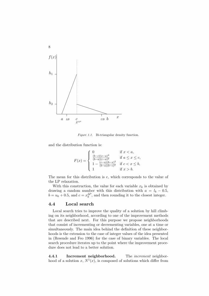
4.3.2 Bi-triangular construction. The goal of this strategyis to increase the diversification of the solutions. In the previous con-struction, we only have two possibilities when we round the value of theLP relaxation of a variable. We here extend this for having the possi-bility of assigning each variable to any integer between its lower-bound,lk, and its upper-bound, uk. The RCL is built with these values, and,again, we give a probability of assignment to each of them based on thesolution of the LP relaxation.
The probability density function that we considered is composed bytwo triangles (bi-triangular distribution) and is defined by three param-eters: the minimum a = lk − 0.5, the maximum b = uk + 0.5, and themean c = xLP
k . The values a and b were considered in order to have anon-zero probability of rounding to lk and uk. The bi-triangular densityfunction is represented in Figure 1.1.
The area of the left triangle is proportional to the distance between cand b and the area of the right triangle is proportional to the distancebetween a and c. The combined areas must be one, since it is a densityfunction. The probability density function is given by:
The mean for this distribution is c, which corresponds to the value ofthe LP relaxation.
With this construction, the value for each variable xk is obtained bydrawing a random number with this distribution with a = lk − 0.5,b = uk + 0.5, and c = xLP
k , and then rounding it to the closest integer.
4.4 Local searchLocal search tries to improve the quality of a solution by hill climb-
ing on its neighborhood, according to one of the improvement methodsthat are described next. For this purpose we propose neighborhoodsthat consist of incrementing or decrementing variables, one at a time orsimultaneously. The main idea behind the definition of these neighbor-hoods is the extension to the case of integer values of the idea presentedin (Resende and Feo 1996) for the case of binary variables. The localsearch procedure iterates up to the point where the improvement proce-dure does not lead to a better solution.
4.4.1 Increment neighborhood. The increment neighbor-hood of a solution x, N1(x), is composed of solutions which differ from
GRASP for linear integer programming 9
x on one element xj , whose value is one unit above or below xj . Hencey is a neighbor solution of x if for one index i, yi = xi +1, or yi = xi−1,with yj = xj for all indices j 6= i:
N1(x) = { y ∈ Z : y can be obtained from x by adding orsubtracting one unit to an element of x}.
The idea used on this neighborhood can be extended to the case wherewe change more than one variable at the same time. For example, the 2-increment neighborhood of a solution x, N2(x), is composed of solutionswhich differ from x on two elements xi and xj , whose values are one unitabove or below the original ones. Hence y is a neighbor solution of x iffor two indices i, j we have yi = xi + 1 or yi = xi − 1, and yj = xj + 1or yj = xj − 1, with yl = xl for all indices l 6= i, l 6= j.
More generally, we can define the k-increment neighborhood (for prob-lems with n ≥ k integer variables) as:
Nk(x) = { y ∈ Z : y can be obtained from x by adding orsubtracting one unit to k of its elements}.
When k increases, the number of neighbors of a solution increasesexponentially. In order to reduce the size of the set of neighbors that ismore frequently explored, we devised the following strategy. Let O bethe set of indices of variables which have coefficients that are differentof zero in the objective function:
O = {i : ci 6= 0, for i = 1, . . . , n}.
Let V (x) be the set of indices of variables (if some) which have coeffi-cients different of zero on constraints violated by x:
V (x) = {j : aij 6= 0, for i ∈ {constraints violated by x}}.
For a solution x, the subset of neighbors with at least one indexin the sets O (for feasible x) or V (x) (for infeasible x) compose theneighborhood Nk∗
(x) ⊆ Nk(x) which is explored first. The subsetNk′
(x) = Nk(x) \ Nk∗(x) is explored when a local optimum of Nk∗
has been found. Neighborhoods Nk are explored in increasing order onk.
This strategy for exploring the neighborhoods is called variable neigh-borhood search (Hansen and Mladenovic 2001). It consists of searchingfirst restricted neighborhoods which are more likely to contain improvingsolutions; when there are no better solutions in a restricted neighbor-hood, this is enlarged, until having explored the whole, unrestrictedneighborhood.
4.4.2 Improvements. There are two methods for updatingthe best solution when searching a particular neighborhood.
The first one, called breadth-first, consists of searching the best solu-tion y in the entire neighborhood of a solution x. If it is better than
10
the current solution x, then x is replaced by y; otherwise, x is a localoptimum. This method will hence search the whole neighborhood of thecurrent solution, even if improving solutions can be found on the earlyexploration of the neighborhood.
The second method, called depth-first, consists of replacing x when-ever the neighbor generated, y, is better than x. In this case, the subse-quent neighbor z is generated from y.
Empirically, the computational time required to obtain a local op-timum is longer with the first method, and premature convergence ismore likely to occur. Therefore, in this implementation the search ismade depth-first.
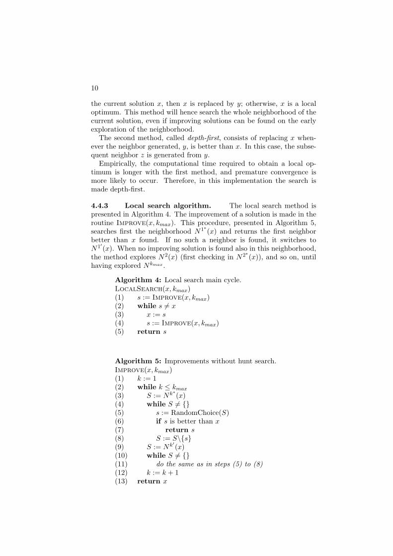
4.4.3 Local search algorithm. The local search method ispresented in Algorithm 4. The improvement of a solution is made in theroutine Improve(x, kmax). This procedure, presented in Algorithm 5,searches first the neighborhood N1∗(x) and returns the first neighborbetter than x found. If no such a neighbor is found, it switches toN1′(x). When no improving solution is found also in this neighborhood,the method explores N2(x) (first checking in N2∗(x)), and so on, untilhaving explored Nkmax .
Algorithm 4: Local search main cycle.LocalSearch(x, kmax)(1) s := Improve(x, kmax)(2) while s 6= x(3) x := s(4) s := Improve(x, kmax)(5) return s
Algorithm 5: Improvements without hunt search.Improve(x, kmax)(1) k := 1(2) while k ≤ kmax
(3) S := Nk∗(x)
(4) while S 6= {}(5) s := RandomChoice(S)(6) if s is better than x(7) return s(8) S := S\{s}(9) S := Nk′
(x)(10) while S 6= {}(11) do the same as in steps (5) to (8)(12) k := k + 1(13) return x
GRASP for linear integer programming 11
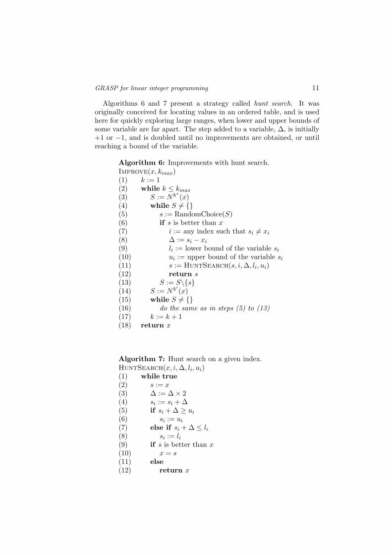
Algorithms 6 and 7 present a strategy called hunt search. It wasoriginally conceived for locating values in an ordered table, and is usedhere for quickly exploring large ranges, when lower and upper bounds ofsome variable are far apart. The step added to a variable, ∆, is initially+1 or −1, and is doubled until no improvements are obtained, or untilreaching a bound of the variable.
Algorithm 6: Improvements with hunt search.Improve(x, kmax)(1) k := 1(2) while k ≤ kmax
(3) S := Nk∗(x)
(4) while S 6= {}(5) s := RandomChoice(S)(6) if s is better than x(7) i := any index such that si 6= xi
(8) ∆ := si − xi
(9) li := lower bound of the variable si
(10) ui := upper bound of the variable si
(11) s := HuntSearch(s, i,∆, li, ui)(12) return s(13) S := S\{s}(14) S := Nk′
(x)(15) while S 6= {}(16) do the same as in steps (5) to (13)(17) k := k + 1(18) return x
Algorithm 7: Hunt search on a given index.HuntSearch(x, i,∆, li, ui)(1) while true(2) s := x(3) ∆ := ∆× 2(4) si := si + ∆(5) if si + ∆ ≥ ui
(6) si := ui
(7) else if si + ∆ ≤ li(8) si := li(9) if s is better than x(10) x = s(11) else(12) return x
12
5. Benchmark problemsLanguages for mathematical programming are the tools more com-
monly used for specifying a model, and generally allow transforming themathematical model into an MPS file. As the heuristic that we describecan be used for any MIP model that can be specified as a mathematicalprogram, we have decided to provide the input to the heuristic throughMPS files. GRASP starts by reading an MPS file, and stores the in-formation contained there into an internal representation. The numberof variables and constraints, their type and bounds, and all the matrixinformation is, hence, determined at runtime.
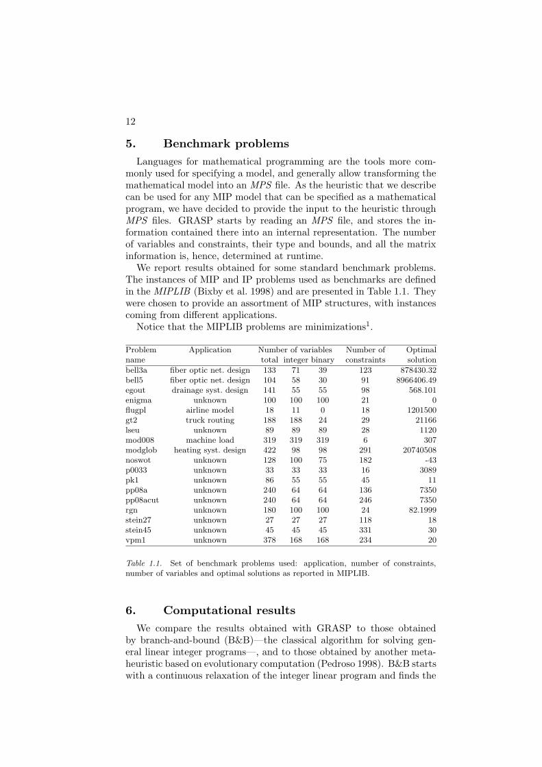
We report results obtained for some standard benchmark problems.The instances of MIP and IP problems used as benchmarks are definedin the MIPLIB (Bixby et al. 1998) and are presented in Table 1.1. Theywere chosen to provide an assortment of MIP structures, with instancescoming from different applications.
Notice that the MIPLIB problems are minimizations1.
Problem Application Number of variables Number of Optimalname total integer binary constraints solution
Table 1.1. Set of benchmark problems used: application, number of constraints,number of variables and optimal solutions as reported in MIPLIB.
6. Computational resultsWe compare the results obtained with GRASP to those obtained
by branch-and-bound (B&B)—the classical algorithm for solving gen-eral linear integer programs—, and to those obtained by another meta-heuristic based on evolutionary computation (Pedroso 1998). B&B startswith a continuous relaxation of the integer linear program and finds the
GRASP for linear integer programming 13
optimal solution by a systematic division of the domain of the relaxedproblem. The evolutionary solver is based on ideas similar to thoseemployed here for solution representation and improvement, but usespopulation-based methods.
The software implementing the branch-and-bound algorithm used inthis experiment is called lp solve (Berkelaar and Dirks). It also comprisesa solver for linear programs based on the simplex method, which wasused both on this GRASP implementation and on (Pedroso 1998) forsolving Equations 1.3 and 1.42. Notice that the LPs solved by GRASPat the time of solution evaluation (if some) are often much simpler thanthose solved by B&B; as all the integer variables are fixed, the size ofthe LPs may be much smaller. Hence, numerical problems that the LPsolver may show up in B&B, do not arise for LPs formulated by GRASP.Therefore, the comparison made in terms of objective evaluations/LPsolutions required favors B&B.
This section begins presenting the results obtained using B&B. Statis-tical measures used in order to assess the empirical efficiency of GRASPare defined next. Follow the results obtained using GRASP, and a com-parison of results of GRASP, B&B, and an evolutionary algorithm.
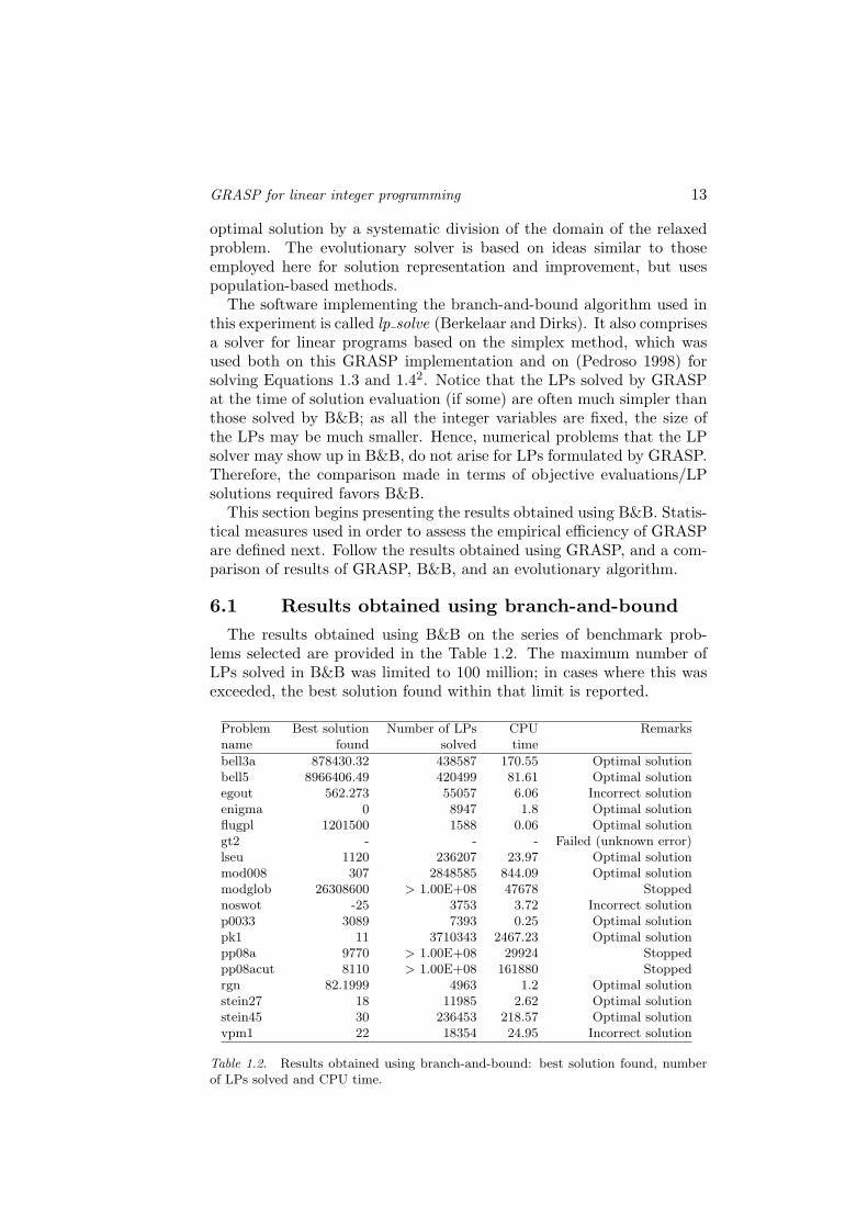
6.1 Results obtained using branch-and-boundThe results obtained using B&B on the series of benchmark prob-
lems selected are provided in the Table 1.2. The maximum number ofLPs solved in B&B was limited to 100 million; in cases where this wasexceeded, the best solution found within that limit is reported.
Problem Best solution Number of LPs CPU Remarksname found solved time
Table 1.2. Results obtained using branch-and-bound: best solution found, numberof LPs solved and CPU time.
14
6.2 Statistical measuresIn order to assess the empirical efficiency of GRASP, we provide mea-
sures of the expectation of the number of LP solutions and CPU timerequired for finding a feasible solution, the best solution found, and theoptimal solution, for MIP problems. These measures are similar for IPproblems, but instead of being developed in terms of the number of LPsolutions, they are made in terms of the number of calls to the objectivefunction (Equations 1.2 or 1.5).
The number of GRASP independent iterations (or runs) for eachbenchmark problem in a given experiment is denoted by N .
6.2.1 Measures in terms of the number of LP solutions.Let rf , rb and ro be the number of runs in which a feasible, the
best, and the optimal solution were found, respectively. Let nfk be the
number of objective evaluations required for obtaining a feasible solutionin iteration k, or the total number of evaluations in that run if no feasiblesolution was found. Identical measures for reaching optimality and thebest solution found by GRASP are denoted by no
k and nbk, respectively.
Then, the expected number of evaluations for reaching feasibility, basedon these N iterations, is:
E[nf ] =N∑
k=1
nfk
rf.
Equivalently, the expected number of evaluations for reaching the bestGRASP solution is
E[nb] =N∑
k=1
nbk
rb,
and the expected number of evaluations for reaching optimality is
E[no] =N∑
k=1
nok
ro.
In case ro = 0, the sum of the evaluations of the total experiment (Niterations) provides a lower bound on the expectations for optimality.The same for feasibility, when rf = 0.
6.2.2 Measures in terms of CPU time. Let tfk be the CPUtime required for obtaining a feasible solution in iteration k, or the totalCPU time in that iteration if no feasible solution was found. Let tok andtbk be identical measures for reaching optimality, and the best solutionfound by GRASP, respectively. Then, the expected CPU time requiredfor reaching feasibility, based on these N iterations, is:
E[tf ] =N∑
k=1
tfkrf
,
GRASP for linear integer programming 15
while
E[tb] =N∑
k=1
tbkrb
is the expected CPU time for finding the best GRASP solution, and theexpected CPU time required for reaching optimality is
E[to] =N∑
k=1
tokro
.
For rf = 0 and ro = 0, the sums provide respectively a lower bound onthe expectations of CPU time required for feasibility and optimality.
6.3 Results obtained using GRASPIn this section we provide a series of results comparing the several
strategies that were implemented: the two construction methods, thek-increment neighborhood (Nk) for k = 1 and k = 2, explored with andwithout hunt search.
The computer environment used on this experiment is the following:a Linux Debian operating system running on a machine with an AMDAthlon processor at 1.4 GHz, with 512 Gb of RAM. GRASP was imple-mented on the C++ programming language.
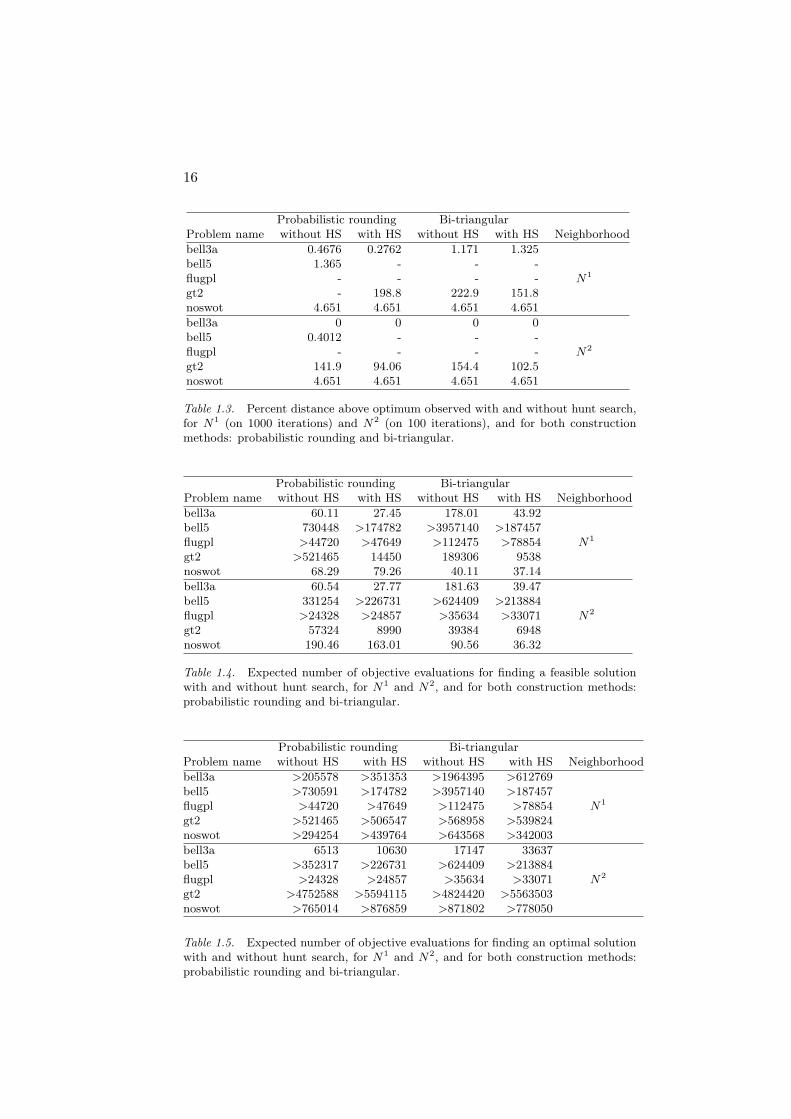
6.3.1 Hunt search. We started making an experiment forassessing the validity of hunt search (HS), with 1000 GRASP iterationswith the 1-increment neighborhood (N1), and 100 iterations with the2-increment neighborhood (N2) (the total time spent in each of thetwo cases is roughly the same). We used both probabilistic roundingconstruction (PRC) and bi-triangular construction (BTC).
We report results obtained for instances with non-binary integer variables—bell3a, bell5, flugpl, gt2 and noswot (hunt search does not apply whenall the integer variables are binary). Table 1.3 reports the percent dis-tance from the best solution found to the optimal solution3, for N1 andN2, respectively (“-” means that the best solution found is not feasi-ble). Table 1.4 reports the expected number of LP solutions/evaluationsfor obtaining feasibility. The same results for obtaining optimality arereported in Table 1.5.
Comparing these two strategies (GRASP with and without hunt search),we conclude that, in general, hunt search slightly improves the results.This improvement is more significant for the bi-triangular construction:as the constructed solutions are more likely to be far away from localoptima, hunt search has more potential for operating.
In the experiments that follow, GRASP was implemented with huntsearch.
16
Probabilistic rounding Bi-triangularProblem name without HS with HS without HS with HS Neighborhood
Table 1.3. Percent distance above optimum observed with and without hunt search,for N1 (on 1000 iterations) and N2 (on 100 iterations), and for both constructionmethods: probabilistic rounding and bi-triangular.
Probabilistic rounding Bi-triangularProblem name without HS with HS without HS with HS Neighborhood
Table 1.4. Expected number of objective evaluations for finding a feasible solutionwith and without hunt search, for N1 and N2, and for both construction methods:probabilistic rounding and bi-triangular.
Probabilistic rounding Bi-triangularProblem name without HS with HS without HS with HS Neighborhood
Table 1.5. Expected number of objective evaluations for finding an optimal solutionwith and without hunt search, for N1 and N2, and for both construction methods:probabilistic rounding and bi-triangular.
GRASP for linear integer programming 17
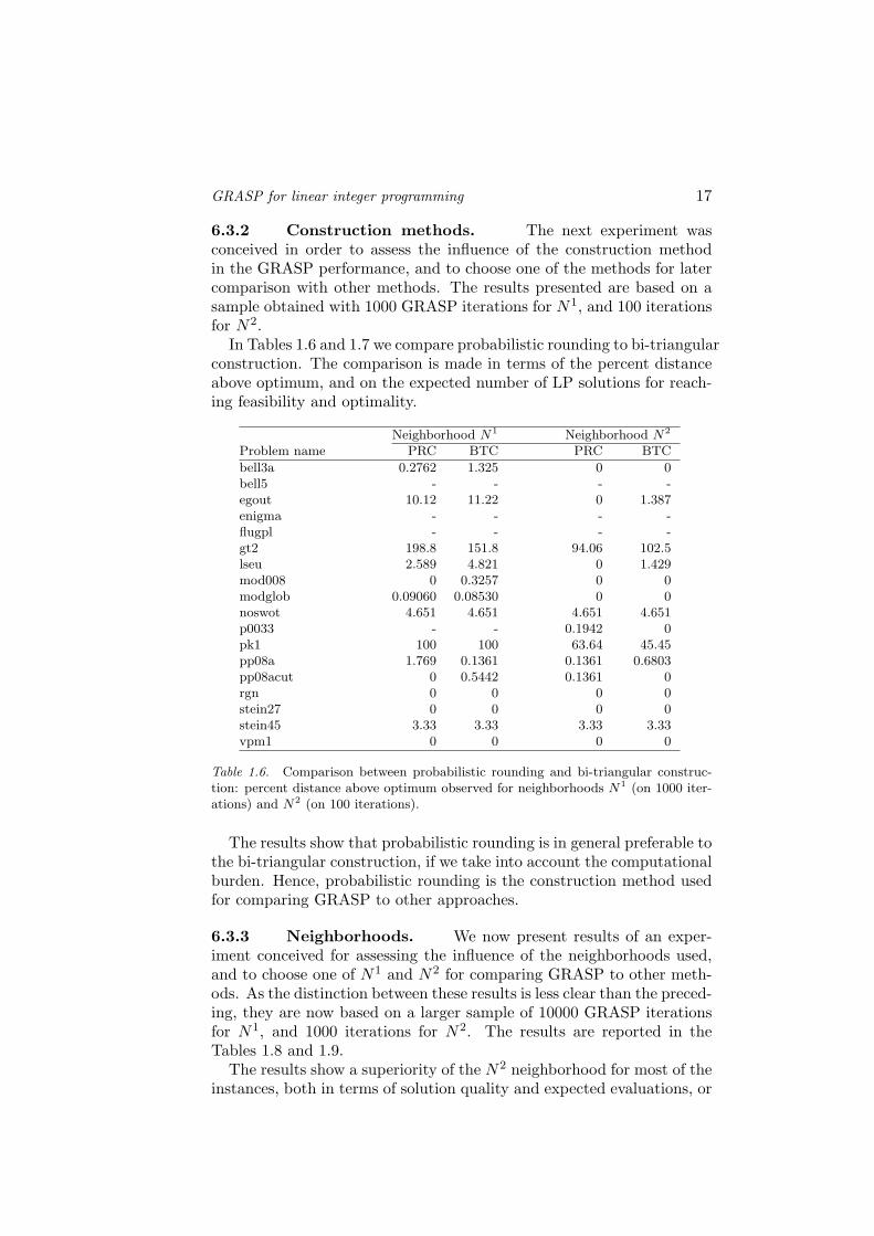
6.3.2 Construction methods. The next experiment wasconceived in order to assess the influence of the construction methodin the GRASP performance, and to choose one of the methods for latercomparison with other methods. The results presented are based on asample obtained with 1000 GRASP iterations for N1, and 100 iterationsfor N2.
In Tables 1.6 and 1.7 we compare probabilistic rounding to bi-triangularconstruction. The comparison is made in terms of the percent distanceabove optimum, and on the expected number of LP solutions for reach-ing feasibility and optimality.
Table 1.6. Comparison between probabilistic rounding and bi-triangular construc-tion: percent distance above optimum observed for neighborhoods N1 (on 1000 iter-ations) and N2 (on 100 iterations).
The results show that probabilistic rounding is in general preferable tothe bi-triangular construction, if we take into account the computationalburden. Hence, probabilistic rounding is the construction method usedfor comparing GRASP to other approaches.
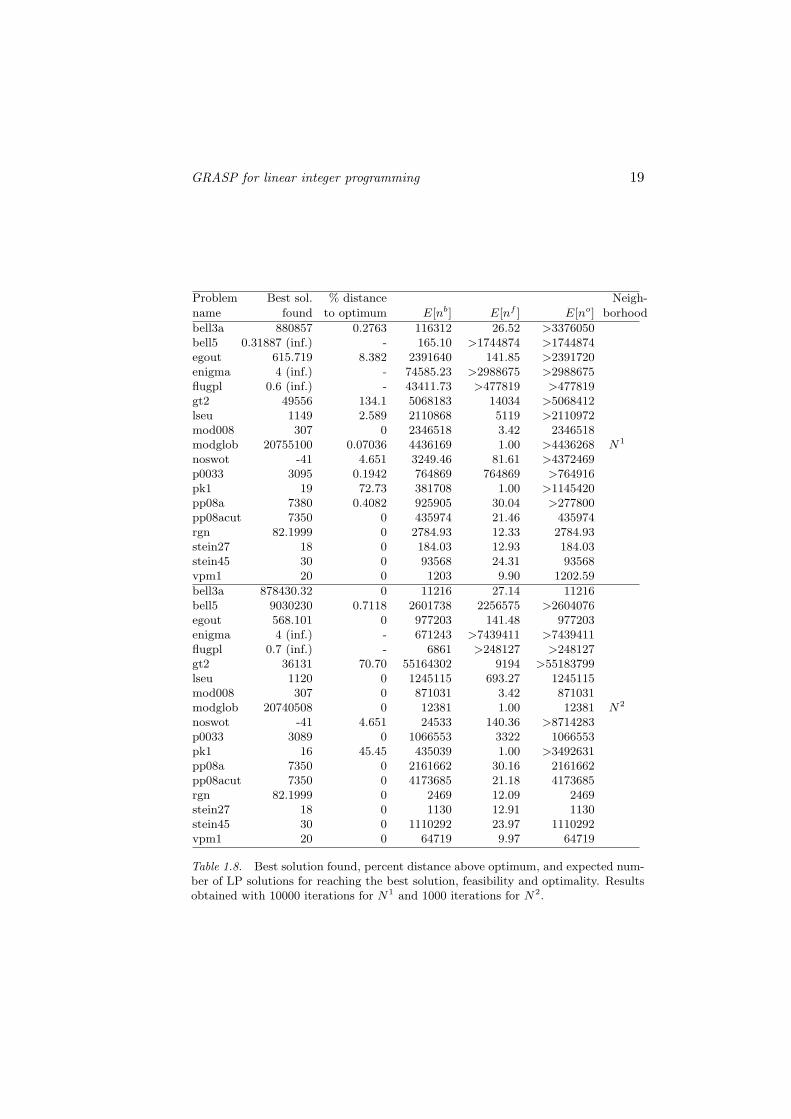
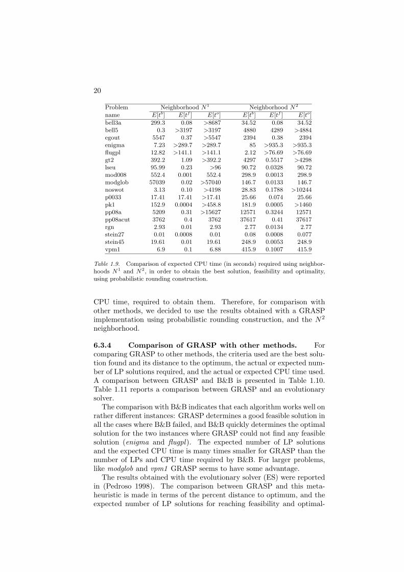
6.3.3 Neighborhoods. We now present results of an exper-iment conceived for assessing the influence of the neighborhoods used,and to choose one of N1 and N2 for comparing GRASP to other meth-ods. As the distinction between these results is less clear than the preced-ing, they are now based on a larger sample of 10000 GRASP iterationsfor N1, and 1000 iterations for N2. The results are reported in theTables 1.8 and 1.9.
The results show a superiority of the N2 neighborhood for most of theinstances, both in terms of solution quality and expected evaluations, or
Table 1.7. Comparison between probabilistic rounding and bi-triangular construc-tion: expected number of objective evaluations for obtaining feasibility and optimal-ity, for neighborhoods N1 and N2.
Table 1.8. Best solution found, percent distance above optimum, and expected num-ber of LP solutions for reaching the best solution, feasibility and optimality. Resultsobtained with 10000 iterations for N1 and 1000 iterations for N2.
Table 1.9. Comparison of expected CPU time (in seconds) required using neighbor-hoods N1 and N2, in order to obtain the best solution, feasibility and optimality,using probabilistic rounding construction.
CPU time, required to obtain them. Therefore, for comparison withother methods, we decided to use the results obtained with a GRASPimplementation using probabilistic rounding construction, and the N2
neighborhood.
6.3.4 Comparison of GRASP with other methods. Forcomparing GRASP to other methods, the criteria used are the best solu-tion found and its distance to the optimum, the actual or expected num-ber of LP solutions required, and the actual or expected CPU time used.A comparison between GRASP and B&B is presented in Table 1.10.Table 1.11 reports a comparison between GRASP and an evolutionarysolver.
The comparison with B&B indicates that each algorithm works well onrather different instances: GRASP determines a good feasible solution inall the cases where B&B failed, and B&B quickly determines the optimalsolution for the two instances where GRASP could not find any feasiblesolution (enigma and flugpl). The expected number of LP solutionsand the expected CPU time is many times smaller for GRASP than thenumber of LPs and CPU time required by B&B. For larger problems,like modglob and vpm1 GRASP seems to have some advantage.
The results obtained with the evolutionary solver (ES) were reportedin (Pedroso 1998). The comparison between GRASP and this meta-heuristic is made in terms of the percent distance to optimum, and theexpected number of LP solutions for reaching feasibility and optimal-
GRASP for linear integer programming 21
Problem GRASP B&B GRASP B&B GRASP B&B
name % to opt. % to opt. E[nb] # LPs E[tb] CPU time
Table 1.10. Comparison between GRASP and B&B: percent distance above opti-mum, expected number of LP solutions and CPU time for GRASP to obtain its bestsolution, and number of LPs and CPU required by B&B.
Problem % dist. to optimum E[nf ] E[no]name GRASP ES GRASP ES GRASP ES
Table 1.11. Comparison between GRASP and an evolutionary solver: percent dis-tance to optimum, and expected number of LP solutions for reaching feasibility andoptimality.
22
ity. The results are reported in Table 1.11. Notice that the terminationcriteria for GRASP and for the ES are very different, and hence the com-parison in terms of distance to optimality is not very meaningful. Still,it shows that the two meta-heuristics have difficulties on roughly thesame instances. This is not surprising, as the ES has an improvementroutine based on a neighborhood similar to N1. On the other hand,the expected times required for obtaining feasibility and optimality canbe dramatically different, indicating that population-based routines andrecombination are a good complement to moves within the neighbor-hoods N1 and N2. Instances where the ES is much slower than GRASPare probably due to the absence of improvements based on N2 on thatsolver, or to the lack of diversity generated by construction on GRASP.(Comparisons based on CPU time were not made, as the ES results wereobtained on very different machines.)
Comparing GRASP to the state-of-the-art commercial solver Xpress-MP Optimizer, Release 13.02 indicated a clear advantage of that solver,which in most cases could find an optimal solution one to four ordersof magnitude faster. Still, this solver had problems on some instances:bell5 and noswot could not be solved in 24 hours of CPU time. Forsome other instances (bell3a, pk1, stein27 ), Xpress-MP required moreLP solutions than GRASP.
7. ConclusionIn this paper we present a GRASP for the solution of integer linear
problems. The algorithm starts by reading an MPS file with the in-stance data. When the problem is a MIP, the integer variables are fixedby GRASP and replaced in the original problem, leading to a pure con-tinuous problem. This problem can be solved by a liner program solver,to evaluate the corresponding fixed variables. When the original prob-lem is an IP, simple algebraic manipulations can be used to evaluate thefixed variables.
The algorithm works with feasible and infeasible solutions. If thesolution is feasible, its evaluation is determined directly by the objectivefunction. If the solution is infeasible, the evaluation is given by the sumof constraint violations, which is determined by solving an LP (for MIPproblems) or by simple algebraic manipulations (for IP problems).
The results obtained with GRASP for some benchmark problems werecompared to those obtained by B&B and to those obtained by an evo-lutionary solver. The comparison with B&B shows that GRASP has avery interesting behavior, as it determines good feasible solutions in thecases where B&B fails. In the comparison with the evolutionary solver,we could verify that the population-based methods used there could leadmany times to substantial reductions on the CPU time required to ob-tain a given solution. On other cases, substantial CPU time reductionsare on the side of GRASP; therefore, no clear conclusion about which
BIBLIOGRAPHY 23
of the meta-heuristics is better could be drawn. GRASP being simpler,it might be the appropriate choice if implementation burden is to beavoided.
Notes1. The GRASP implementation works for minimization and maximization, by adapting
the meaning of is better (see section 4.2.4).
2. This software has the advantage of being free; on the other hand, it does not havesome important components, like the dual simplex method, which would allow to quicklyreoptimize Equation 1.3 from a dual solution after a change in the right hand side.
3. Let fb be the objective value for the best feasible solution, and fo for the optimalsolution. The percent distance above the optimum is given by
˛100× (fb − fo)/fo
˛.
BibliographyMichel R. Berkelaar and Jeroen Dirks. lp solve - a solver for linear
programming problems with a callable subroutine library. Internetrepository, version 2.2. ftp://ftp.es.ele.tue.nl/pub/lp solve.
S. Binato, W. J. Henry, D. Loewenstern, and M. G. C. Resende. A greedyrandomized adaptive search procedure for job scheduling. In C. C.Ribeiro and P. Hansen, editors, Essays and surveys on metaheuristics.Kluwer Academic Publishers, 2001.
Robert E. Bixby, Sebastian Ceria, Cassandra M. McZeal, and MartinW. P. Savelsbergh. An updated mixed integer programming library.Technical report, Rice University, 1998. TR98-03.
C. Carreto and B. Baker. A GRASP interactive approach to the vehi-cle routing problem with backhauls. In C. C. Ribeiro and P. Hansen,editors, Essays and Surveys on Metaheuristics. Kluwer Academic Pub-lishers, 2001.
T. A. Feo and M. G. C. Resende. A probabilistic heuristic for a computa-cionally difficult set covering problem. Operations Research Letters,8:67–71, 1989.
T. A. Feo and M. G. C. Resende. Greedy randomized adaptive searchprocedures. J. of Global Optimization, 6:109–133, 1995.
T. A. Feo, K. Venkatraman, and J. F. Bard. A GRASP for a difficultsingle machine sheduling problem. Computers & Operations Research,18:635–643, 1991.
P. Festa and M. G. C. Resende. GRASP: an annotated bibliography. InC. C. Ribeiro and P. Hansen, editors, Essays and Surveys on Meta-heuristics. Kluwer Academic Publishers, 2001.
Pierre Hansen and Nenad Mladenovic. Variable neighborhood search:Principles and applications. European Journal of Operational Re-search, 130:449–467, 2001.
24
G. Kontoravdis and J. F. Bard. A GRASP for the vehicle routing prob-lem with time windows. ORSA J. on Computing, 7:10–23, 1995.
Thomas Lengauer. Combinatorial Algorithms for Integrated Circuit Lay-out, chapter 8, pages 427–446. Applicable Theory in Computer Sci-ence. John Wiley and Sons, 1990.
Y. Li, P. M. Pardalos, and M. G. C. Resende. A greedy randomizedadaptive search procedure for the quadratic assignment problem. InP.M. Pardalos and H. Wolkowicz, editors, Quadratic assignment andrelated problems, volume 16 of DIMACS Series on Discrete Mathe-matics and Theoretical Computer Science, pages 237–261. AmericanMathematical Society, 1994.
George L. Nemhauser and Laurence A. Wolsey. Integer and Combina-torial Optimization. Wiley-Interscience in Discrete Mathematics andOptimization, 1988.
Joao P. Pedroso. An evolutionary solver for linear integer programming.BSIS Technical Report 98-7, Riken Brain Science Institute, Wako-shi,Saitama, Japan, 1998.
Joao P. Pedroso. An evolutionary solver for pure integer linear pro-gramming. International Transactions in Operational Research, 9(3):337–352, May 2002.
L. S. Pitsoulis and M. G. C. Resende. Greedy randomized adaptivesearch procedures. In P. M. Pardalos and M. G. C. Resende, editors,Handbook of Applied Optimization, pages 168–183. Oxford UniversityPress, 2002.
M. G. C. Resende and T. A. Feo. A GRASP for satisfiability. In D. S.Johnson and M. A. Trick, editors, Cliques, Coloring and Satisfiabil-ity: The second DIMACS Implementation Challenge, volume 26 ofDIMACS Series on Discrete Mathematics and Theoretical ComputerScience, pages 499–520. American Mathematical Society, 1996.
M. G. C. Resende, L. S. Pitsoulis, and P. M. Pardalos. Approximate so-lution of weighted MAX-SAT problems using GRASP. In Satisfiabilityproblems, volume 35 of DIMACS Series on Discrete Mathematics andTheoretical Computer Science, pages 393–405. American Mathemati-cal Society, 1997.
M. G. C. Resende and C. C. Ribeiro. Greedy randomized adaptive searchprocedure. In Fred Glover and G. Kochenberger, editors, State of theArt Handbook in Metaheuristics. Kluwer Academic Publishers, 2001.
A.J. Robertson. A set of greedy randomized adaptive local search proce-dure (GRASP) implementations for the multidimensional assignment
BIBLIOGRAPHY 25
problem. Computational Optimization and Applications, 19:145–164,2001.
Laurence A. Wolsey. Integer Programming. Wiley-Interscience in Dis-crete Mathematics and Optimization, 1998.