Chapter 1Introduction and Kinetics of Particles

1.1 Introduction

There are two main approaches in simulating the transport equations (heat, mass, andmomentum), continuum and discrete. In continuum approach, ordinary or partialdifferential equations can be achieved by applying conservation of energy, mass, andmomentum for an infinitesimal control volume. Since it is difficult to solve thegoverning differential equations for many reasons (nonlinearity, complex boundaryconditions, complex geometry, etc.), therefore finite difference, finite volume, finiteelement, etc., schemes are used to convert the differential equations with a givenboundary and initial conditions into a system of algebraic equations. The algebraicequations can be solved iteratively until convergence is insured. Let us discuss theprocedure in more detail, first the governing equations are identified (mainly partialdifferential equation). The next step is to discretize the domain into volume, girds, orelements depending on the method of solution. We can look at this step as eachvolume or node or element contains a collection of particles (huge number, order of1016). The scale is macroscopic. The velocity, pressure, temperature of all thoseparticles represented by a nodal value, or averaged over a finite volume, or simplyassumed linearly or bi-linearly varied from one node to another. The phenomeno-logical properties such as viscosity, thermal conductivity, heat capacity, etc. are ingeneral known parameters (input parameters, except for inverse problems). Forinverse problems, one or more thermophysical properties may be unknown.

On the other extreme, the medium can be considered made of small particles(atom, molecule) and these particles collide with each other. This scale is micro-scale. Hence, we need to identify the inter-particle (inter-molecular) forces andsolve ordinary differential equation of Newton’s second law (momentum conser-vation). At each time step, we need to identify location and velocity of eachparticle, i.e, trajectory of the particles. At this level, there is no definition oftemperature, pressure, and thermo-physical properties, such as viscosity, thermalconductivity, heat capacity, etc. For instance, temperature and pressure are relatedto the kinetic energy of the particles (mass and velocity) and frequency of particles

A. A. Mohamad, Lattice Boltzmann Method,DOI: 10.1007/978-0-85729-455-5_1, � Springer-Verlag London Limited 2011

1

bombardment on the boundaries, respectively. This method is called moleculardynamics (MD) simulations. To get an idea, a number of equations need to besolved; 103 cm of air at the room conditions contains about 3� 1022 molecules.One mole of water (16 g, a small cup of water) contains more than 6:0� 1023

molecules. To visualize this number, if we assume that the diameter of thesemolecules is 1 mm (tip of a pen, a dot) and these dots are arranged side by side,then the total area that can be covered by these dots is 6:0� 1011 km2: The totalsurface area of the earth is about 5:1� 109 km2 and area of the United States is9:63� 106 km2 and area of Africa is 1:22� 106 km2: This means that we cancover the total area of the earth by dots made from number of molecules of 16 g ofwater if the molecule diameter is 1 mm. Furthermore, it is interesting to calculatehow many years we need to complete the project of doting the world by using pentip. For a reasonable fast person, 6 dots per second is a good estimate. Hence, itneeds at least about 3� 1015 years to complete the project.

The question is do we really need to know the behavior of each molecule oratom?

In bookkeeping process we need to identify location (x; y; z) and velocity (cx; cy;

and cz are velocity components in x; y and z direction, respectively) of each par-ticle. Also, the simulation time step should be less than the particles collision time,which is in the order of fero-seconds (10�12 s). Hence, it is impossible to solvelarge size problems (order of cm) by MD method. At this scale, there is nodefinition of viscosity, thermal conductivity, temperature, pressure, and otherphenomenological properties. Statistical mechanics need to be used as a translatorbetween the molecular world and the macroscopic world. The question is, is thevelocity and location of each particle important for us? For instance, in this roomthere are billions of molecules traveling at high speed order of 400 m/s; likerockets, hitting us. But, we do not feel them, because their mass (momentum) is sosmall. The resultant effect of such a ‘‘chaotic’’ motion is almost nil, where the airin the room is almost stagnant (i.e., velocity in the room is almost zero). Hence, thebehavior of the individual particles is not an important issue on the macroscopicscale, the important thing is the resultant effects.

Fundamentally, MD is simple and can handle phase change and complexgeometries without any difficulties and without introducing extra ingredients.However, it is important to specify the appropriate inter-particle force function.The main drawback or obstacle of using MD in simulation of a relatively largesystem is the computer resource and data reduction process, which will not beavailable for us in the seen future.

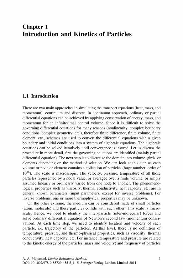
What about a middle man, sitting at the middle of both mentioned techniques,the lattice Boltzmann method (LBM). The main idea of Boltzmann is to bridge thegap between micro-scale and macro-scale by not considering each particlebehavior alone but behavior of a collection of particles as a unit, Fig. 1.1. Theproperty of the collection of particles is represented by a distribution function. Thekeyword is the distribution function. The distribution function acts as a repre-sentative for collection of particles. This scale is called meso-scale.

2 1 Introduction and Kinetic of Particles

The mentioned methods are illustrated in Fig. 1.1.LBM enjoys advantages of both macroscopic and microscopic approaches, with

manageable computer resources.LBM has many advantages. It is easy to apply for complex domains, easy to

treat multi-phase and multi-component flows without a need to trace the interfacesbetween different phases. Furthermore, it can be naturally adapted to parallelprocesses computing. Moreover, there is no need to solve Laplace equation at eachtime step to satisfy continuity equation of incompressible, unsteady flows, as it isin solving Navier–Stokes (NS) equation. However, it needs more computermemory compared with NS solver, which is not a big constraint. Also, it canhandle a problem in micro- and macro-scales with reliable accuracy.

1.2 Kinetic Theory

It is necessary to be familiar with the concepts and terminology of kinetic theorybefore proceeding to LBM. The following sections are intended to introduce thereader to the basics and fundamentals of kinetic theory of particles. I tried to avoidthe detail of mathematics; however more emphasis is given to the physics.

Continuum( Macroscopic scale), finite difference, finite volume, finite element, etc),

Navier-Stokes Equations

Lattice Boltzmann Method(Mesoscopic scale),

Boltzmann Equation

Molecular Dynamics (Microscopic scale),

Hamilton s Equation.

Fig. 1.1 Techniques of simulations

1.1 Introduction 3

Note that, the word particle and molecule are used interchangeably in thefollowing paragraphs.

1.2.1 Particle Dynamics

As far as we know, the main building block of all the materials in nature is themolecules and sub-molecules. These molecules can be visualized as solid spheresmoving ‘‘randomly’’ in conservatory manner in a free space. The motion satisfiesconservation of the mass, momentum, and energy. Hence, Newton’s second law(momentum conservation) can be applied, which states that the rate of change oflinear momentum is equal to the net applied force.

F ¼ dðmcÞdt

ð1:1Þ

where F stands for the inter-molecular and external forces, m is the mass of theparticle, c is the velocity vector of the particle and t is the time. For a constantmass, the equation can be simplified as,

F ¼ mdc

dt¼ ma ð1:2Þ

where a is the acceleration vector. The position of the particle can be determinedfrom definition of velocity,

c ¼ dr

dtð1:3Þ

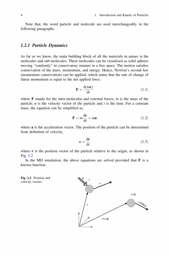
where r is the position vector of the particle relative to the origin, as shown inFig. 1.2

In the MD simulation, the above equations are solved provided that F is aknown function.

Fig. 1.2 Position andvelocity vectors

4 1 Introduction and Kinetic of Particles

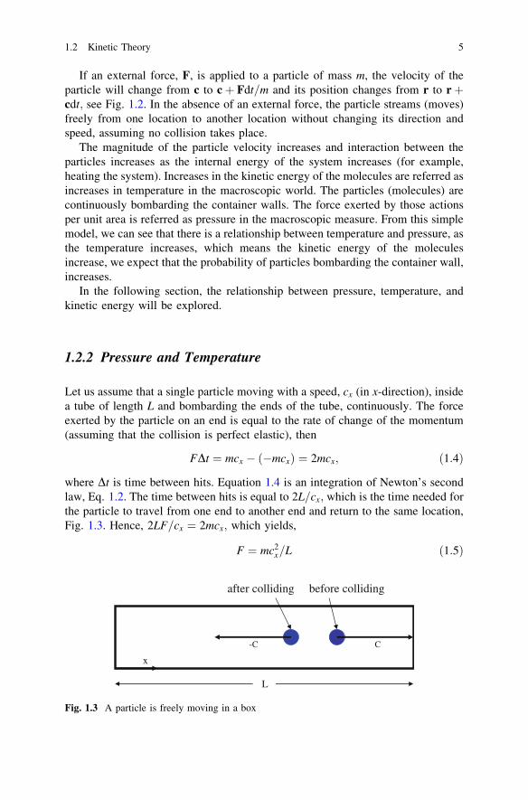
If an external force, F, is applied to a particle of mass m, the velocity of theparticle will change from c to cþ Fdt=m and its position changes from r to rþcdt; see Fig. 1.2. In the absence of an external force, the particle streams (moves)freely from one location to another location without changing its direction andspeed, assuming no collision takes place.

The magnitude of the particle velocity increases and interaction between theparticles increases as the internal energy of the system increases (for example,heating the system). Increases in the kinetic energy of the molecules are referred asincreases in temperature in the macroscopic world. The particles (molecules) arecontinuously bombarding the container walls. The force exerted by those actionsper unit area is referred as pressure in the macroscopic measure. From this simplemodel, we can see that there is a relationship between temperature and pressure, asthe temperature increases, which means the kinetic energy of the moleculesincrease, we expect that the probability of particles bombarding the container wall,increases.

In the following section, the relationship between pressure, temperature, andkinetic energy will be explored.

1.2.2 Pressure and Temperature

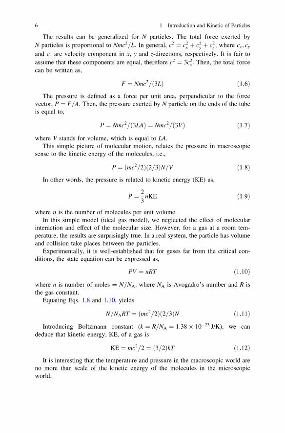
Let us assume that a single particle moving with a speed, cx (in x-direction), insidea tube of length L and bombarding the ends of the tube, continuously. The forceexerted by the particle on an end is equal to the rate of change of the momentum(assuming that the collision is perfect elastic), then

FDt ¼ mcx � ð�mcxÞ ¼ 2mcx; ð1:4Þ

where Dt is time between hits. Equation 1.4 is an integration of Newton’s secondlaw, Eq. 1.2. The time between hits is equal to 2L=cx; which is the time needed forthe particle to travel from one end to another end and return to the same location,Fig. 1.3. Hence, 2LF=cx ¼ 2mcx; which yields,

F ¼ mc2x=L ð1:5Þ

after colliding before colliding

L

-C C

x

Fig. 1.3 A particle is freely moving in a box

1.2 Kinetic Theory 5

The results can be generalized for N particles. The total force exerted byN particles is proportional to Nmc2=L: In general, c2 ¼ c2

x þ c2y þ c2

z ; where cx; cy

and cz are velocity component in x, y and z-directions, respectively. It is fair toassume that these components are equal, therefore c2 ¼ 3c2

x : Then, the total forcecan be written as,

F ¼ Nmc2=ð3LÞ ð1:6Þ

The pressure is defined as a force per unit area, perpendicular to the forcevector, P ¼ F=A: Then, the pressure exerted by N particle on the ends of the tubeis equal to,

P ¼ Nmc2=ð3LAÞ ¼ Nmc2=ð3VÞ ð1:7Þ

where V stands for volume, which is equal to LA.This simple picture of molecular motion, relates the pressure in macroscopic

sense to the kinetic energy of the molecules, i.e.,

P ¼ ðmc2=2Þð2=3ÞN=V ð1:8Þ

In other words, the pressure is related to kinetic energy (KE) as,

P ¼ 23

nKE ð1:9Þ

where n is the number of molecules per unit volume.In this simple model (ideal gas model), we neglected the effect of molecular

interaction and effect of the molecular size. However, for a gas at a room tem-perature, the results are surprisingly true. In a real system, the particle has volumeand collision take places between the particles.

Experimentally, it is well-established that for gases far from the critical con-ditions, the state equation can be expressed as,

PV ¼ nRT ð1:10Þ

where n is number of moles = N=NA; where NA is Avogadro’s number and R isthe gas constant.

Equating Eqs. 1.8 and 1.10, yields

N=NART ¼ ðmc2=2Þð2=3ÞN ð1:11Þ

Introducing Boltzmann constant (k ¼ R=NA ¼ 1:38� 10�23 J/K), we candeduce that kinetic energy, KE, of a gas is

KE ¼ mc2=2 ¼ ð3=2ÞkT ð1:12Þ

It is interesting that the temperature and pressure in the macroscopic world areno more than scale of the kinetic energy of the molecules in the microscopicworld.

6 1 Introduction and Kinetic of Particles

1.3 Distribution Function

In 1859, Maxwell (1831–1879) recognized that dealing with a huge number ofmolecules is difficult to formulate, even though the governing equation (Newton’ssecond law) is known. As mentioned before, tracing the trajectory of each mol-ecule is out of hand for a macroscopic system. Then, the idea of averaging cameinto picture. For illustration purposes, in a class of 500 students (extremely smallnumber, compared with the number of molecules in volume of 1 mm3), if all thestudents started asking a question simultaneously, the result is noise and chaos.However, the question can be addressed through a class representative, which canbe handled easily and the result may be acceptable by the majority.

The idea of Maxwell is that the knowledge of velocity and position of eachmolecule at every instant of time is not important. The distribution function is theimportant parameter to characterize the effect of the molecules; what percentage ofthe molecules in a certain location of a container have velocities within a certainrange, at a given instant of time. The molecules of a gas have a wide range ofvelocities colliding with each others, the fast molecules transfer momentum to theslow molecule. The result of the collision is that the momentum is conserved. For agas in thermal equilibrium, the distribution function is not a function of time,where the gas is distributed uniformly in the container; the only unknown is thevelocity distribution function.

For a gas of N particles, the number of particles having velocities in the x-direction between cx and cx þ dcx is Nf ðcxÞdcx: The function f ðcxÞ is the fractionof the particles having velocities in the interval cx and cx þ dcx; in the x-direction.Similarly, for other directions, the probability distribution function can be definedas before. Then, the probability for the velocity to lie down between cx andcx þ dcx; cy and cy þ dcy; and cz and cz þ dcz will be Nf ðcxÞf ðcyÞf ðczÞdcxdcydcz:

It is important to mention that if the above equation is integrated (summed) overall possible values of the velocities, yields the total number of particles to be N,i.e.,

ZZZf ðcxÞf ðcyÞf ðczÞ dcx dcy dcz ¼ 1: ð1:13Þ

Since any direction can be x, or y or z, the distribution function should notdepend on the direction, but only on the speed of the particles. Therefore,

f ðcxÞf ðcyÞf ðczÞ ¼ Uðc2x þ c2

y þ c2z Þ ð1:14Þ

where U is another unknown function, that need to be determined. The value ofdistribution function should be positive (between zero and unity). Hence, inEq. 1.14, velocity is squared to avoid negative magnitude. The possible functionthat has property of Eq. 1.14 is logarithmic or exponential function, i.e.,

1.3 Distribution Function 7

log Aþ log B ¼ logðABÞ ð1:15Þ

or

eAeB ¼ eðAþBÞ ð1:16Þ

It can be shown that the appropriate form for the distribution function should beas,

f ðcxÞ ¼ Ae�Bc2x ð1:17Þ

where A and B are constants. The exponential function implies that the multipli-cation of the functions can be added if each function is equal to the exponent of afunction.

For example:

FðxÞ ¼ eBx; FðyÞ ¼ eCy;

then

FðxÞFðyÞ ¼ eBxeCy ¼ eðBxþCyÞ:

But if FðxÞ ¼ Bx and FðyÞ ¼ Cy; then FðxÞFðyÞ ¼ BxCy; in this case themultiplication of function is not equal to the addition of the functions. Accord-ingly, it can be assumed that,

f ðcÞ ¼ Ae�Bc2x Ae�Bc2

y Ae�Bc2z ¼ A3e�Bc2 ð1:18Þ

Multiplying together the probability distributions for the three directions,gives the distribution in terms of the particle speed c. In other words, the dis-tribution function is that giving the number of particles having speed betweenc and cþ dc:

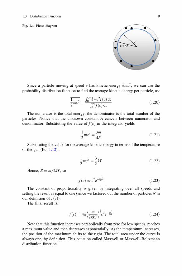
It is important to think about the distribution of particles in velocity space, athree-dimensional space (cx; cy; cz), where each particle is represented by a pointhaving coordinates corresponding to the particle’s velocity. Thus, all points lyingon a spherical surface centered at the origin correspond to the same speed.Therefore, the number of particles having speed between c and cþ dc equals thenumber of points lying between two shells of the sphere, with radii c and cþ dc;Fig. 1.4.

The volume of the spherical shell is 4pc2dc: Therefore, the probability distri-bution as a function of speed is:

f ðcÞdc ¼ 4pc2A3e�Bc2dc ð1:19Þ

Integration of above function for the given Fig. 1.4 yields eight particles.The constants A and B can be determined by integrating the probability dis-

tribution over all possible speeds to find the total number of particles N, and theirtotal energy E.

8 1 Introduction and Kinetic of Particles

Since a particle moving at speed c has kinetic energy 12 mc2; we can use the

probability distribution function to find the average kinetic energy per particle, as:

12

mc2 ¼R1

012 mc2f ðcÞ dcR10 f ðcÞ dc

ð1:20Þ

The numerator is the total energy, the denominator is the total number of theparticles. Notice that the unknown constant A cancels between numerator anddenominator. Substituting the value of f ðcÞ in the integrals, yields

12

mc2 ¼ 3m

4Bð1:21Þ

Substituting the value for the average kinetic energy in terms of the temperatureof the gas (Eq. 1.12),

12

mc2 ¼ 32

kT ð1:22Þ

Hence, B ¼ m=2kT ; so

f ðcÞ / c2e�mc22kT ð1:23Þ

The constant of proportionality is given by integrating over all speeds andsetting the result as equal to one (since we factored out the number of particles N inour definition of f ðcÞ).

The final result is:

f ðcÞ ¼ 4pm

2pkT

� �32c2e�

mc22kT ð1:24Þ

Note that this function increases parabolically from zero for low speeds, reachesa maximum value and then decreases exponentially. As the temperature increases,the position of the maximum shifts to the right. The total area under the curve isalways one, by definition. This equation called Maxwell or Maxwell–Boltzmanndistribution function.

Fig. 1.4 Phase diagram

1.3 Distribution Function 9

The probability of finding a particle that has a specific velocity is zero, becausethe velocity of particles change continuously over a wide range. The meaningfulquestion is to find the probability of a particle or particles within a range ofvelocity rather than at a specific velocity. Therefore, Eq. 1.24, need to be inte-grated in that range of velocity.

Example For air molecules (say, nitrogen) at 0 and 100�C temperatures, calculatethe distribution function.

The mass of one molecule of N2; which is molar mass (28 g/mol or 0.028 kg/mol) divided by Avogadro’s number (6:022� 1023 mol�1) gives 4:6496180671�10�26 kg; which is mass of one N2 molecule. The Boltzmann constant is 1:38�10�23 J/K ðkg m2=ðs2 KÞ:

Then m=ð2kÞ ¼ 4:6496180671� 10�3=ð2 � 1:38Þ ¼ 1:684644227� 10�3

ðm2=ðs2 KÞÞ: h

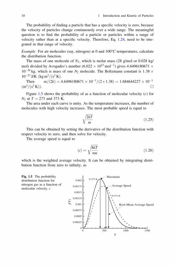
Figure 1.5 shows the probability of as a function of molecular velocity (c) forN2 at T ¼ 273 and 373 K.

The area under each curve is unity. As the temperature increases, the number ofmolecules with high velocity increases. The most probable speed is equal to

ffiffiffiffiffiffiffiffi2kT

m

rð1:25Þ

This can be obtained by setting the derivative of the distribution function withrespect velocity to zero, and then solve for velocity.

The average speed is equal to

hci ¼ffiffiffiffiffiffiffiffi8kT

pm

rð1:26Þ

which is the weighted average velocity. It can be obtained by integrating distri-bution function from zero to infinity, as

V

f(V

)

0 500 1000 15000

0.00025

0.0005

0.00075

0.001

0.00125

0.0015

0.00175

0.002 T=273 K

T=373 K

Average Speed

Root-Mean-Average Speed

MaximumFig. 1.5 The probabilitydistribution function fornitrogen gas as a function ofmolecular velocity, c

10 1 Introduction and Kinetic of Particles

hci ¼Z1

0

cf ðcÞ dc ð1:27Þ

The root-mean-average speed is equal to

hc2i ¼Z1

0

c2f ðcÞ dc ¼ 3kT

mð1:28Þ

The mean average speed is equal to ðc2x þ c2

y þ c2z Þ

1=2 and average speed isequal to ðcx þ cy þ czÞ=3:

The root mean squared speed of a molecule is

crms ¼ffiffiffiffiffiffiffiffihc2i

p¼

ffiffiffiffiffiffiffiffiffiffiffi3KBT

m

rð1:29Þ

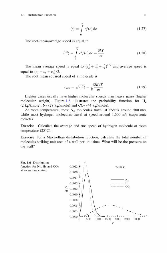
Lighter gases usually have higher molecular speeds than heavy gases (highermolecular weight). Figure 1.6 illustrates the probability function for H2

(2 kg/kmole), N2 (28 kg/kmole) and CO2 (44 kg/kmole).At room temperature, most N2 molecules travel at speeds around 500 m/s,

while most hydrogen molecules travel at speed around 1,600 m/s (supersonicrockets).

Exercise Calculate the average and rms speed of hydrogen molecule at roomtemperature (25�C).

Exercise For a Maxwellian distribution function, calculate the total number ofmolecules striking unit area of a wall per unit time. What will be the pressure onthe wall?

V

f(V

)

0 500 1000 1500 2000 2500 30000.0000

0.0003

0.0005

0.0008

0.0010

0.0012

0.0015

0.0017

0.0020

0.0022

N2

H2

CO2

T=298 K

Fig. 1.6 Distributionfunction for N2; H2 and CO2

at room temperature

1.3 Distribution Function 11

1.3.1 Boltzmann Distribution

Boltzmann generalized the Maxwell’s distribution for arbitrary large systems. Hewas the first to realize the deep connection between the thermodynamic concept ofentropy and the statistical analysis of possible states of a large system—that theincrease in entropy of a system with time is a change in macroscopic variables tothose values corresponding to the largest possible number of microscopicarrangements. Boltzmann showed that the numbers of available microscopic statesfor a given energy are far greater for macroscopic values corresponding to thermalequilibrium. For example, for a given energy there are far more possible micro-scopic arrangements of gas molecules in which the gas is essentially uniformlydistributed in a box than that of all the gas molecules being on the left-hand half ofthe box. Thus, if a liter of gas over the course of time goes through all possiblemicroscopic arrangements, in fact there is a negligible probability of it all being inthe left-hand half in a time the age of the universe. So if we arrange for all theparticles to be in the left-hand half by using a piston to push them there, thenremove the piston, they will rapidly tend to a uniform distribution spread evenlythroughout the box.

Boltzmann proved that the thermodynamic entropy S, of a system (at a givenenergy E) is related to the number W, of microscopic states available to it byS ¼ k logðWÞ; k being Boltzmann’s constant. There were some ambiguities incounting the number of possible microscopic arrangements which were rathertroublesome, but not fatal to the program. For example, how many differentvelocities can a particle in a box have? This matter was cleared up by the quantummechanics.

Boltzmann was then able to establish that for any system large or small inthermal equilibrium at temperature T, the probability of being in a particular state

at energy E is proportional to e�EkT ; i.e.

f ðEÞ ¼ Ae�E=kT ð1:30Þ

This is called the Boltzmann distribution.Let us consider kinetic energy of molecules in x-direction, then

E ¼ 12

mc2x ð1:31Þ

For a normalized probability function, the probability function integrated for allvalues of velocity (from minus to plus infinity) should be one.

Hence,

Z1

�1

Ae�mc2

x2kT dc ¼ 1 ð1:32Þ

Therefore,

12 1 Introduction and Kinetic of Particles

A ¼ffiffiffiffiffiffiffiffiffiffiffi

m

2pkT

rð1:33Þ

The probability of finding velocity cx is

f ðcxÞ ¼ffiffiffiffiffiffiffiffiffiffiffi

m

2pkT

re�

mc2x

2kT ð1:34Þ

We are interested on probability of three dimensional velocity (c) where

c2 ¼ c2x þ c2

y þ c2z ð1:35Þ

The probability of (c) is multiple of probability of each function, i.e.,

f ðcÞ ¼ f ðcxÞf ðcyÞf ðczÞ ð1:36Þ

which leads to

f ðcÞ ¼ffiffiffiffiffiffiffiffiffiffiffi

m

2pkT

r� �3

e�m

2kTðc2xþc2

yþc2z Þ ð1:37Þ

or

f ðcÞ ¼ m

2pkT

� �3=2e�

mc22kT ð1:38Þ

It should be noted that the above equation does not take into account the factthat there are more ways to achieve a higher velocity. In making the step from thisexpression to the Maxwell speed distribution, this distribution function must bemultiplied by the factor 4pc2 (which is surface area of a sphere in the phase space)to account for the density of velocity states available to particles. Therefore,Maxwell distribution function (Eq. 1.24) is covered. In fact, integration of Max-well distribution function (Eq. 1.24) over a surface of sphere in phase space yieldsEq. 1.37.

An ideal gas has a specific distribution function at equilibrium (Maxwell dis-tribution function). But Maxwell did not mention, how the equilibrium is reached.This was one of the revolutionary contribution of Boltzmann, which is the base ofthe LBM.

In the next chapter, Boltzmann transport equation, which is a main concern ofthis book, will be discussed.

1.3 Distribution Function 13