Chapter 1 Systems and Signals Continuous-Time and Discrete-Time Signals Classification of Signals Transformations of the Independent Variables Exponential and Sinusoidal Signals Unit Impulse and Unit Step Functions Continuous-Time and Discrete-Time Systems Basic System Properties Summary
Transcript
Chapter 1 Systems and Signals
Continuous-Time and Discrete-Time Signals
Classification of Signals
Transformations of the Independent Variables
Exponential and Sinusoidal Signals
Unit Impulse and Unit Step Functions
Continuous-Time and Discrete-Time Systems
Basic System Properties
Summary
1. Signals
Signals
Any physical quantity that varies with time, space or any other
independent variable.
Signals are represented mathematically as functions of one
or more independent variables.
In this course, time is usually the only independent variable.
Continuous-time signals are defined for every value of time.
Discrete -time signals are defined at discrete values of time.
2. Classification of Signals
Periodic Signals
2. Classification of Signals
Even and Odd Signals
Even signal: x(-t)=x(t) or x[-n]=x[n]
Odd signal: x(-t)=-x(t) or x[-n]=-x[n]
Any signal can be broken into a sum of an even signal
and an odd signal
x[n] = xe[n] + xo[n]
])[][(2
1][ nxnxnxe
])[][(2
1][ nxnxnxo
2. Classification of Signals
2. Classification of Signals
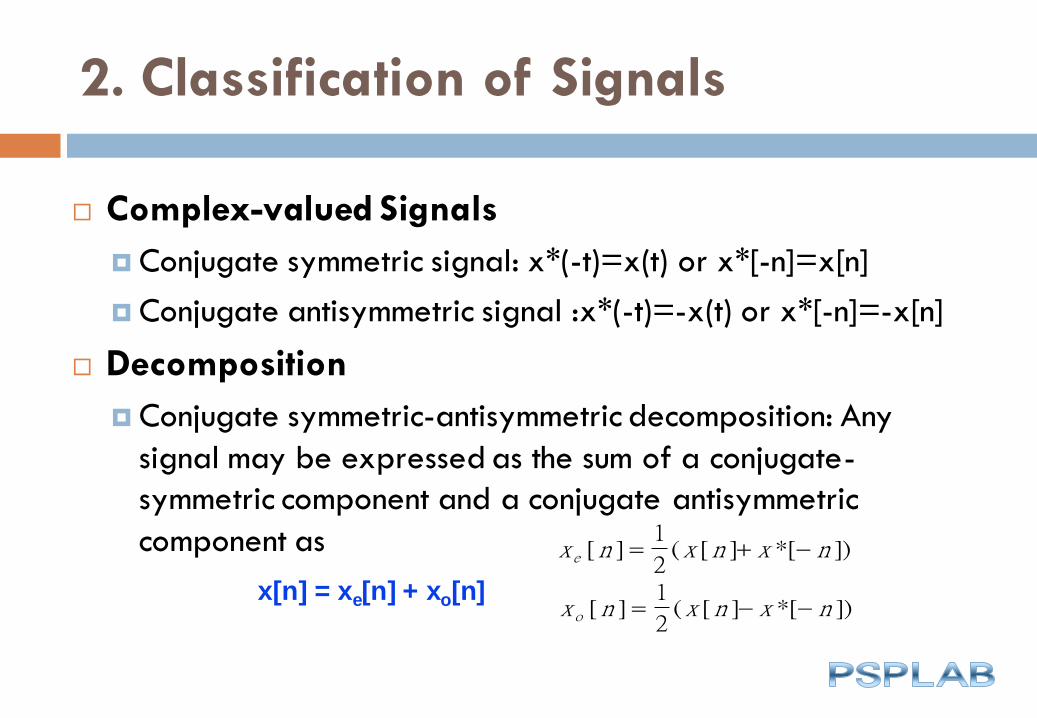
Complex-valued Signals
Conjugate symmetric signal: x*(-t)=x(t) or x*[-n]=x[n]
Conjugate antisymmetric signal :x*(-t)=-x(t) or x*[-n]=-x[n]
Decomposition
Conjugate symmetric-antisymmetric decomposition: Any
signal may be expressed as the sum of a conjugate-
symmetric component and a conjugate antisymmetric
component as
x[n] = xe[n] + xo[n]
x n x n x ne [ ] ( [ ] *[ ]) 1
2
x n x n x no [ ] ( [ ] *[ ]) 1
2
2. Classification of Signals
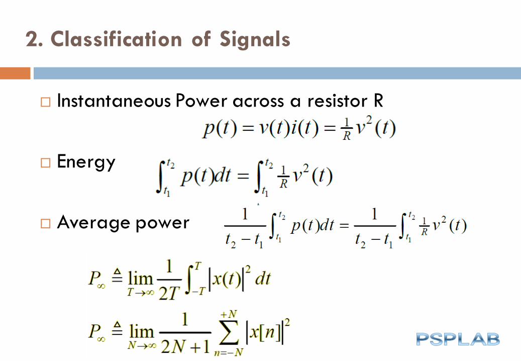
Instantaneous Power across a resistor R
Energy
Average power
2. Classification of Signals
The total energy is defined as
Time Averaged, Power is defined as
dttxdttxE
T
TT)()(lim 2
2/
2/
2
2/
2/
2 )(1
limT
TTdttx
TP
2. Classification of Signals
Signal Energy and Power
Energy signal: A signal for which 0<E<
Power signal: A signal for which 0<P<
If P= , or if E= but P=0, then the signal is neither
energy signal nor power signal
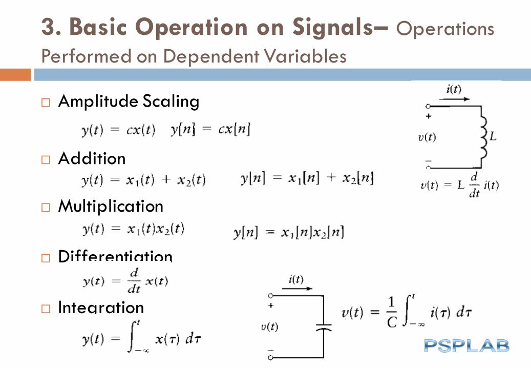
3. Basic Operation on Signals– Operations
Performed on Dependent Variables
Amplitude Scaling
Addition
Multiplication
Differentiation
Integration
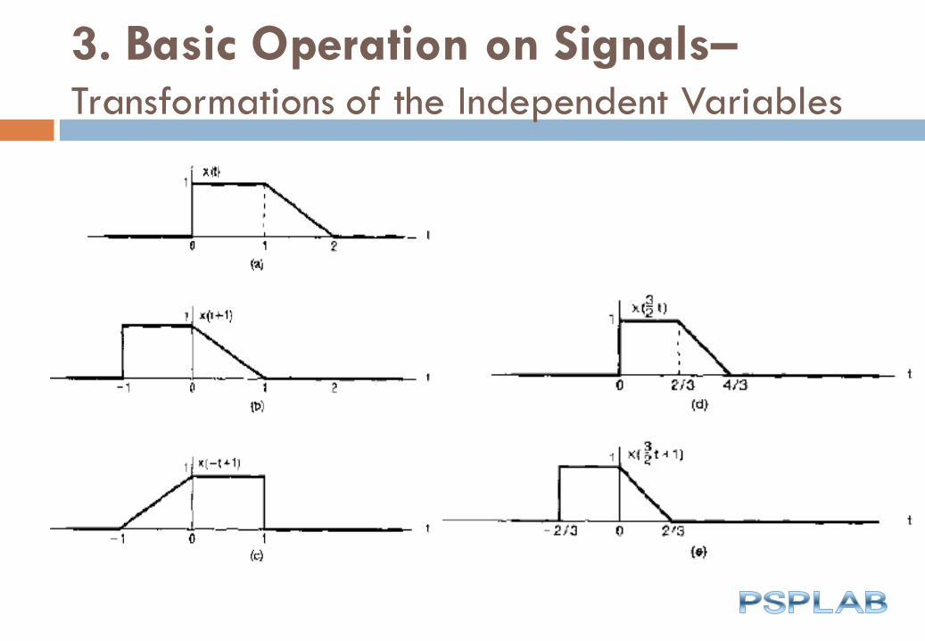
3. Basic Operation on Signals--Transformations of the Independent Variables
Time Shift
3. Basic Operation on Signals–
Transformations of the Independent Variables
Time Reversal
3. Basic Operation on Signals–Transformations of the Independent Variables
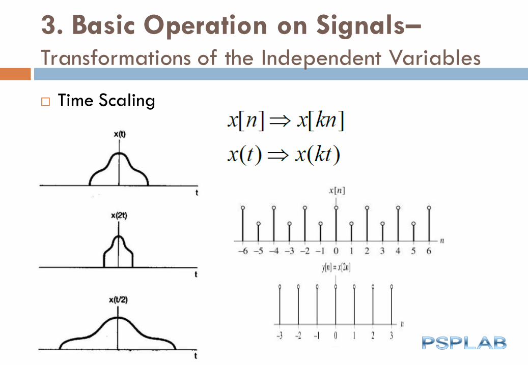
Time Scaling
3. Basic Operation on Signals–Transformations of the Independent Variables
4. Exponential and Sinusoidal Signals
Real Exponential Signals
4. Exponential and Sinusoidal Signals
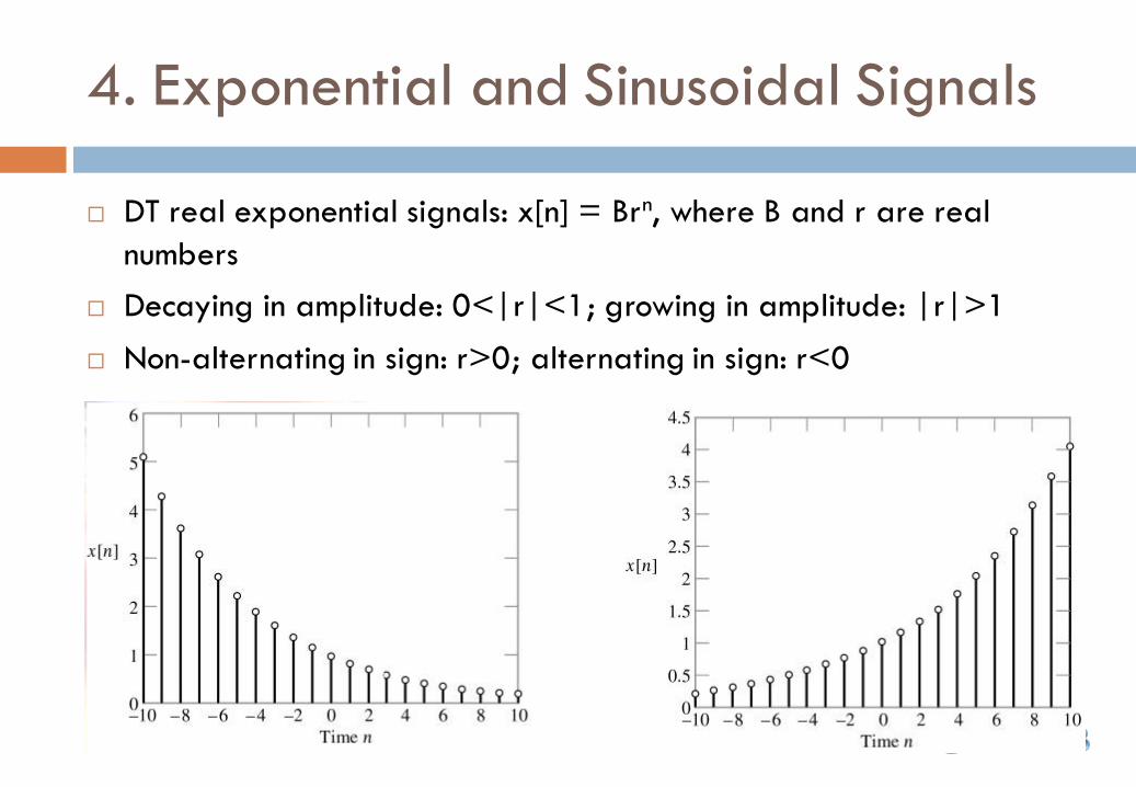
DT real exponential signals: x[n] = Brn, where B and r are real
numbers
Decaying in amplitude: 0<|r|<1; growing in amplitude: |r|>1
Non-alternating in sign: r>0; alternating in sign: r<0
4. Exponential and Sinusoidal Signals
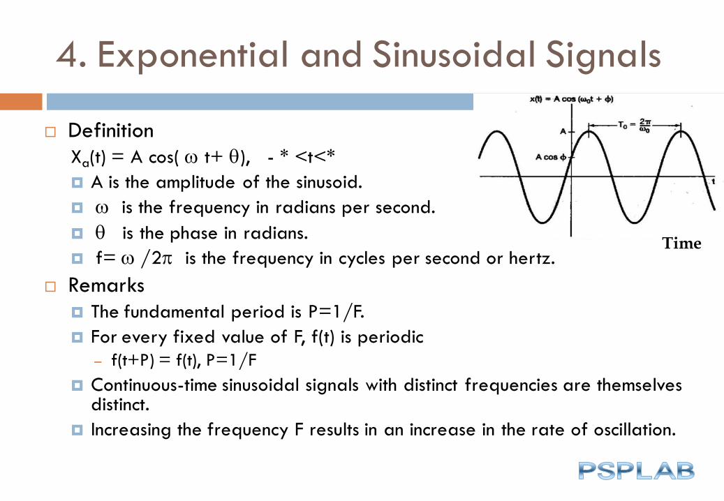
Definition
Xa(t) = A cos( t+ ), - * <t<*
A is the amplitude of the sinusoid.
is the frequency in radians per second.
is the phase in radians.
f= /2p is the frequency in cycles per second or hertz.
Remarks
The fundamental period is P=1/F.
For every fixed value of F, f(t) is periodic
– f(t+P) = f(t), P=1/F
Continuous-time sinusoidal signals with distinct frequencies are themselves distinct.
Increasing the frequency F results in an increase in the rate of oscillation.
Time
4. Exponential and Sinusoidal Signals
CT Complex Exponential Signals
Euler’s Identity
4. Exponential and Sinusoidal Signals
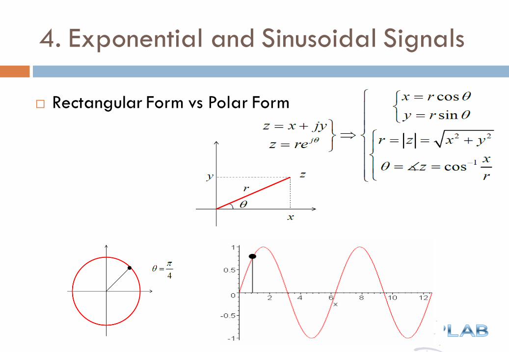
Rectangular Form vs Polar Form
4. Exponential and Sinusoidal Signals
Discrete-Time Form
4. Exponential and Sinusoidal Signals
Discrete-Time Sinusoidal Signals
x(n) = A cos( n+ ), n =1, 2, ...
A is the amplitude of the sinusoid
is the frequency in radians per sample
is the phase in radians
f= /2p is the frequency in cycles per sample or hertz
X(n) = A cos( n+ )
4. Exponential and Sinusoidal Signals
A discrete-time sinsoidal is periodic only if its frequency f is a rational number
– x(n+N) = x(n), N=m/f, where m, N are integers.
Discrete-time sinusoidals where frequencies are separated by an integer multiple of 2p are identical
– x1(n) = A cos( 0 n)
– x2(n) = A cos( (0 2p) n) The highest rate of oscillation in a discrete-time
sinusoidal is attained when =p or (=-p), or equivalently f=1/2.
– X(n) = A cos(( 0+p)n) = -A cos((0+p)n
Discrete-Time Sinusoidal SignalsX(n) = A cos( n+ )
4. Exponential and Sinusoidal Signals
5. Unit Impulse and Unit Step Functions
Unit Impulse Signals
5. Unit Impulse and Unit Step Functions
Dirac Delta function, δ(t), often referred to as the unit
impulse or delta function, is the function that defines the
idea of an unit impulse.
This function is one that is infinitely narrow, infinitely tall,
yet integrates to unity,
5. Unit Impulse and Unit Step Functions
Unit Step Signals
5. Unit Impulse and Unit Step Functions
Perhaps the simplest way to visualize this is
as a rectangular pulse from a−ε/2 to a+ε/2
with a height of 1/ε.
As we take the limit of this, lim 0, we see that
the width tends to zero and the height tends
to infinity as the total area remains constant
at one.
The impulse function is often written as δ(t) .
)(lim)(0
txt
)(tx
2/ 2/
5. Unit Impulse and Unit Step Functions
Properties
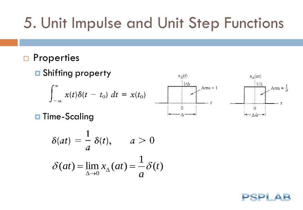
5. Unit Impulse and Unit Step Functions
Properties
Shifting property
Time-Scaling
)(1
)(lim)(0
ta
atxat
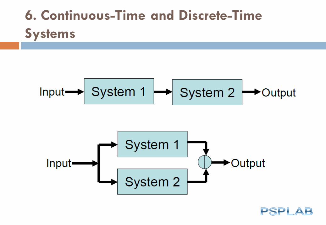
6. Continuous-Time and Discrete-Time
Systems
6. Continuous-Time and Discrete-Time
Systems
6. Continuous-Time and Discrete-Time
Systems
7. Basic System Properties
Systems
Mathematically a transformation or an operator that maps
an input signal into an output signal
Can be either hardware or software.
Such operations are usually referred as signal processing.
E.x.
Discrete-Time System H
n n
y n x k x k x n y n x nk
n
k
n
( ) ( ) ( ) ( ) ( ) ( )
1 1
7. Basic System Properties
Types of Systems
CT systems: input and output are CT signals
DT systems: input and output are DT signals
Mixed systems: CT-in and DT-out (e.g., A/D converter), DT-in
and CT-out (e.g., D/A converter)
7. Basic System Properties
Time-Invariant versus Time-Variant Systems
A system H is time-invariant or shift invariant if and only if
x(n) ---> y(n)
implies that
x(n-k) --> y(n-k)
for every input signal x(n) x(n) and every time shift k.
Causal versus Noncausal Systems
The output at any time depends on values of the input at only the present and past time.
y(n) = F[x(n), x(n-1), x(n-2), ...].
where F[.] is some arbitrary function.
7. Basic System Properties
Linear versus Nonlinear Systems
A system H is linear if and only if
H[a1x1(n)+ a2 x2 (n)] = a1H[x1 (n)] + a2H[x2 (n)]
for any arbitrary input sequences x1(n) and
x2(n), and any arbitrary constants a1 and a2.
Multiplicative or Scaling Property
H[ax(n)] = a H[x(n)]
Additivity Property
H[x1(n) + x2 (n)] = H[x1 (n)] + H[x2 (n)]
Linear systems
y(n)
u1(n)
+
u2(n)
a
b
Linear systems
u1(n)
u2(n)
Linear systems
+y(n)
a
b
7. Basic System Properties
Stable versus Unstable Systems
An arbitrary relaxed system is said to be bounded-input-
bounded-output (BIBO) stable if and only if every bounded
input produces a bounded output.
Ex.
y(t)=tx(t)
y(t)=ex(t)
7. Basic System Properties
Memory versus Memoryless Systems
A system is referred to as memoryless system if the output for
each value of the independent variable depends only on the