1 = 2 ?. ANOVA. Chapter 10 Comparisons Involving Means. Estimation of the Difference between the Means of Two Populations: Independent Samples Hypothesis Tests about the Difference between the Means of Two Populations: Independent Samples - PowerPoint PPT Presentation
54
Chapter 10 Chapter 10 Comparisons Involving Means Comparisons Involving Means 1 1 = = 2 2 ? ? ANOVA ANOVA Estimation of the Difference between the Means of Estimation of the Difference between the Means of Two Populations: Independent Samples Two Populations: Independent Samples Hypothesis Tests about the Difference between the Hypothesis Tests about the Difference between the Means of Two Populations: Independent Means of Two Populations: Independent Samples Samples Inferences about the Difference between the Means Inferences about the Difference between the Means of Two Populations: Matched Samples of Two Populations: Matched Samples Introduction to Analysis of Variance (ANOVA) Introduction to Analysis of Variance (ANOVA) ANOVA: Testing for the Equality of ANOVA: Testing for the Equality of k k Population Population Means Means
Transcript
Chapter 10Chapter 10 Comparisons Involving Means Comparisons Involving Means
11 = = 22 ? ?
ANOVAANOVA
Estimation of the Difference between the Means of Estimation of the Difference between the Means of Two Populations: Independent Samples Two Populations: Independent Samples Hypothesis Tests about the Difference between theHypothesis Tests about the Difference between the Means of Two Populations: Independent SamplesMeans of Two Populations: Independent Samples Inferences about the Difference between the Means Inferences about the Difference between the Means of Two Populations: Matched Samplesof Two Populations: Matched Samples Introduction to Analysis of Variance (ANOVA)Introduction to Analysis of Variance (ANOVA) ANOVA: Testing for the Equality of ANOVA: Testing for the Equality of kk Population Population
MeansMeans
Estimation of the Difference Between the Estimation of the Difference Between the Means of Two Populations: Independent Means of Two Populations: Independent
SamplesSamples Point Estimator of the Difference between the Point Estimator of the Difference between the
Means of Two PopulationsMeans of Two Populations Sampling DistributionSampling Distribution Interval Estimate of Interval Estimate of Large-Sample CaseLarge-Sample Case Interval Estimate of Interval Estimate of Small-Sample CaseSmall-Sample Case
x x1 2
Point Estimator of the Difference BetweenPoint Estimator of the Difference Betweenthe Means of Two Populationsthe Means of Two Populations
Let Let 11 equal the mean of population 1 and equal the mean of population 1 and 22 equal the mean of population 2.equal the mean of population 2.
The difference between the two population The difference between the two population means is means is 11 - - 22..
To estimate To estimate 11 - - 22, we will select a simple , we will select a simple random sample of size random sample of size nn11 from population 1 and from population 1 and a simple random sample of size a simple random sample of size nn22 from from population 2.population 2.
Let equal the mean of sample 1 and equal Let equal the mean of sample 1 and equal the mean of sample 2.the mean of sample 2.
The point estimator of the difference between The point estimator of the difference between the means of the populations 1 and 2 is .the means of the populations 1 and 2 is .
x x1 2
x1 x2
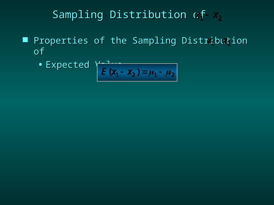
Properties of the Sampling Distribution of Properties of the Sampling Distribution of • Expected ValueExpected Value
Sampling Distribution of Sampling Distribution of x x1 2
x x1 2
E x x( )1 2 1 2
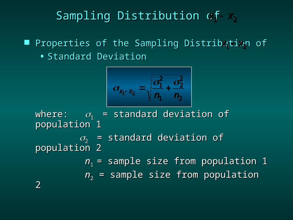
Properties of the Sampling Distribution of Properties of the Sampling Distribution of • Standard DeviationStandard Deviation
where: where: 1 1 = standard deviation of population = standard deviation of population 11
2 2 = standard deviation of = standard deviation of population 2population 2
nn1 1 = sample size from population 1= sample size from population 1 nn22 = sample size from population 2 = sample size from population 2
Sampling Distribution of Sampling Distribution of x x1 2
x x1 2
x x n n1 2
12
1
22
2
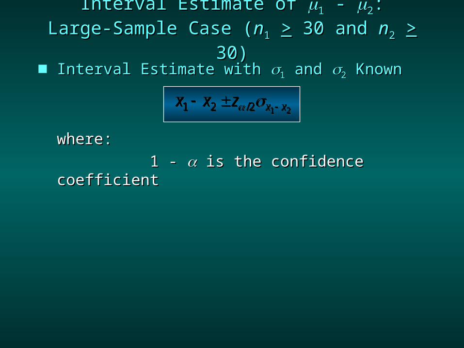
Interval Estimate with Interval Estimate with 11 and and 22 Known Known
where:where:1 - 1 - is the confidence coefficient is the confidence coefficient
Interval Estimate of Interval Estimate of 11 - - 22::Large-Sample Case (Large-Sample Case (nn11 >> 30 and 30 and nn22 >> 30) 30)
x x z x x1 2 2 1 2 /
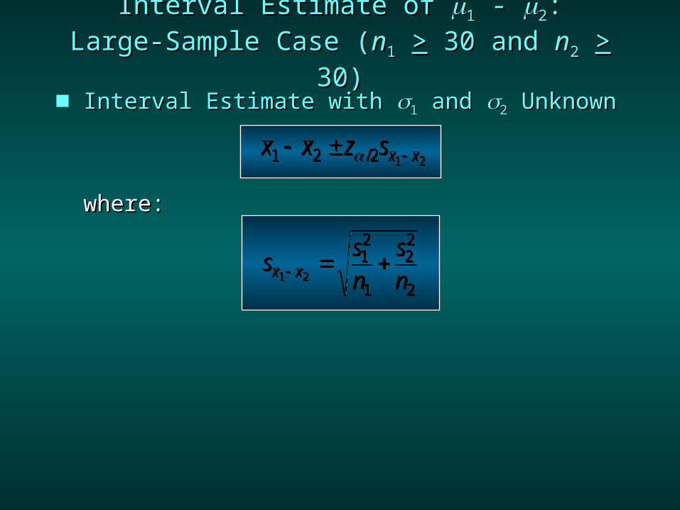
Interval Estimate with Interval Estimate with 11 and and 22 Unknown Unknown
where:where:
Interval Estimate of Interval Estimate of 11 - - 22::Large-Sample Case (Large-Sample Case (nn11 >> 30 and 30 and nn22 >> 30) 30)
x x z sx x1 2 2 1 2 /
s sn
snx x1 2
12
1
22
2
Example: Par, Inc.Example: Par, Inc.
Interval Estimate of Interval Estimate of 11 - - 22: Large-Sample Case: Large-Sample Case Par, Inc. is a manufacturer of golf Par, Inc. is a manufacturer of golf
equipment and has developed a new golf ball equipment and has developed a new golf ball that has been designed to provide “extra that has been designed to provide “extra distance.” In a test of driving distance using a distance.” In a test of driving distance using a mechanical driving device, a sample of Par golf mechanical driving device, a sample of Par golf balls was compared with a sample of golf balls balls was compared with a sample of golf balls made by Rap, Ltd., a competitor. made by Rap, Ltd., a competitor.
The sample statistics appear on the next The sample statistics appear on the next slide.slide.
Example: Par, Inc.Example: Par, Inc.
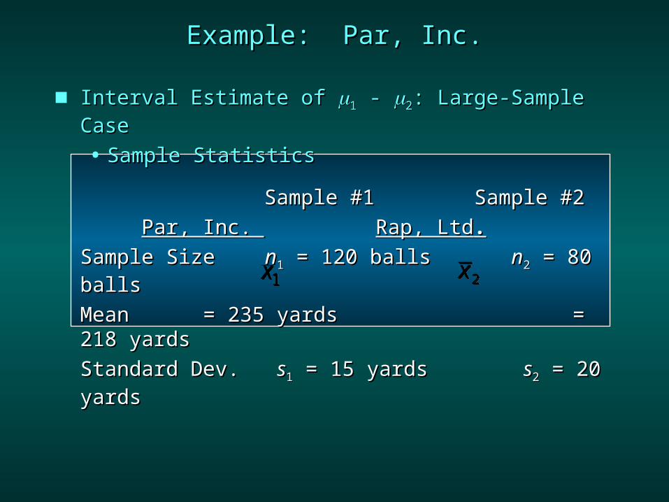
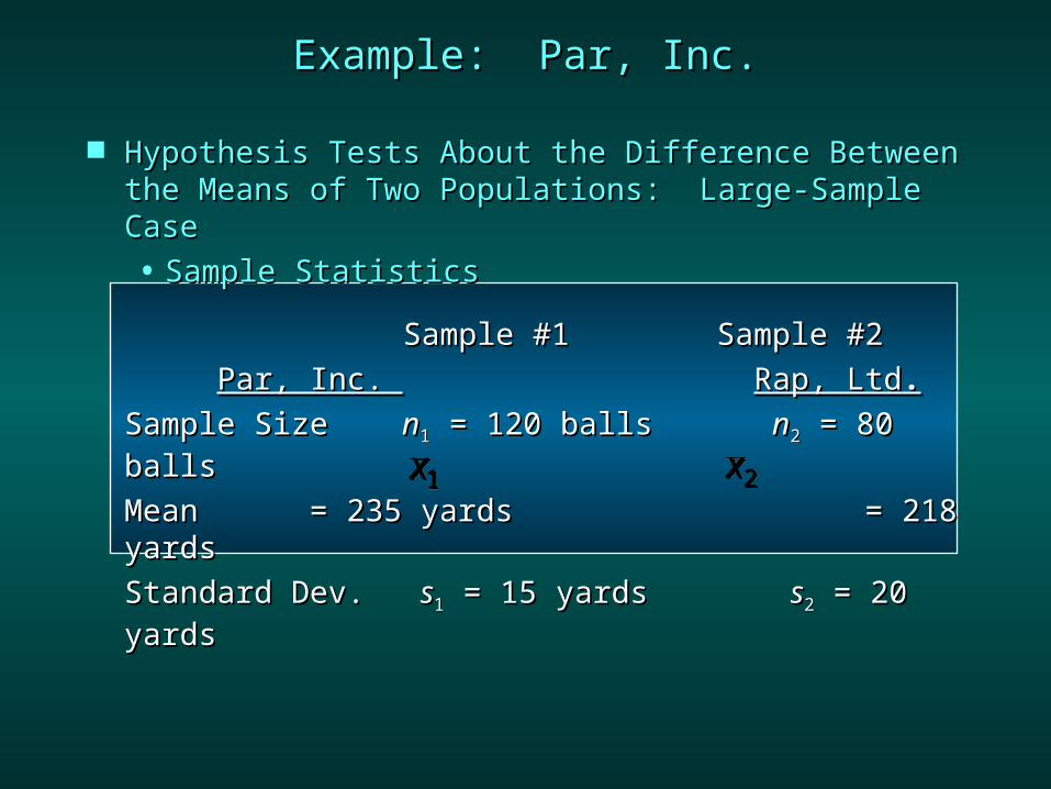
Interval Estimate of Interval Estimate of 11 - - 22: Large-Sample Case: Large-Sample Case • Sample StatisticsSample Statistics
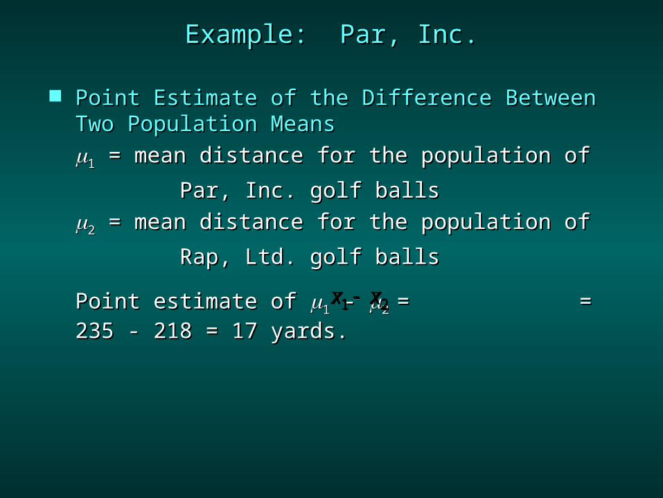
Point Estimate of the Difference Between Two Point Estimate of the Difference Between Two Population MeansPopulation Means
11 = mean distance for the population of = mean distance for the population of Par, Inc. golf ballsPar, Inc. golf balls22 = mean distance for the population of = mean distance for the population of Rap, Ltd. golf ballsRap, Ltd. golf balls
Point estimate of Point estimate of 11 - - 2 2 = = 235 - 218 = = = 235 - 218 = 17 yards.17 yards.
x x1 2
Example: Par, Inc.Example: Par, Inc.
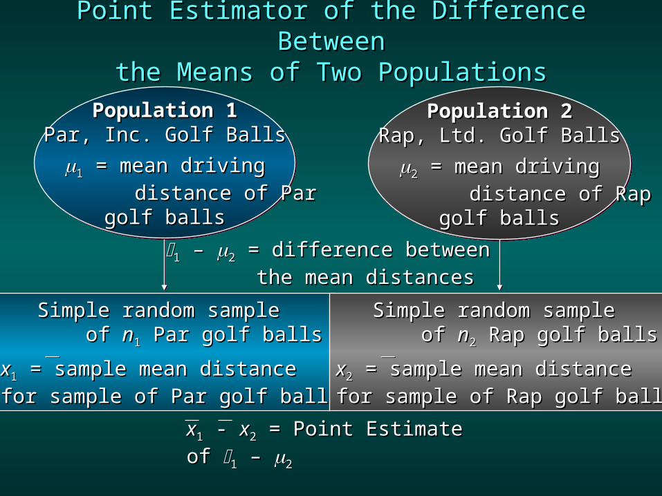
Point Estimator of the Difference BetweenPoint Estimator of the Difference Betweenthe Means of Two Populationsthe Means of Two Populations
Population 1Population 1Par, Inc. Golf BallsPar, Inc. Golf Balls11 = mean driving = mean driving
distance of Pardistance of Pargolf ballsgolf balls
Population 2Population 2Rap, Ltd. Golf BallsRap, Ltd. Golf Balls22 = mean driving = mean driving
distance of Rapdistance of Rapgolf ballsgolf balls
11 – – 22 = difference between= difference between the mean distancesthe mean distances
Simple random sampleSimple random sample of of nn11 Par golf balls Par golf ballsxx11 = sample mean distance = sample mean distancefor sample of Par golf ballfor sample of Par golf ball
Simple random sampleSimple random sample of of nn22 Rap golf balls Rap golf ballsxx22 = sample mean distance = sample mean distancefor sample of Rap golf ballfor sample of Rap golf ball
xx11 - - xx22 = Point Estimate of = Point Estimate of 11 –– 22
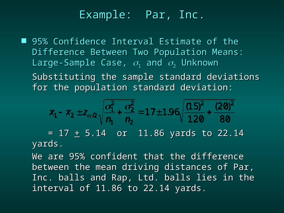
95% Confidence Interval Estimate of the 95% Confidence Interval Estimate of the Difference Between Two Population Means: Difference Between Two Population Means: Large-Sample Case, Large-Sample Case, 11 and and 22 Unknown UnknownSubstituting the sample standard deviations for Substituting the sample standard deviations for the population standard deviation:the population standard deviation:
= 17 = 17 ++ 5.14 or 11.86 yards to 22.14 yards. 5.14 or 11.86 yards to 22.14 yards.We are 95% confident that the difference We are 95% confident that the difference between the mean driving distances of Par, Inc. between the mean driving distances of Par, Inc. balls and Rap, Ltd. balls lies in the interval of balls and Rap, Ltd. balls lies in the interval of 11.86 to 22.14 yards.11.86 to 22.14 yards.
x x zn n1 2 212
1
22
2
2 217 1 96 15
1202080
/ . ( ) ( )
Example: Par, Inc.Example: Par, Inc.
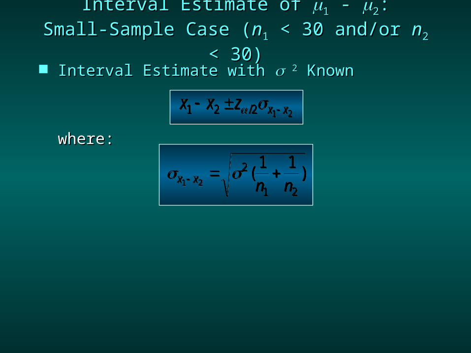
Interval Estimate of Interval Estimate of 11 - - 22::Small-Sample Case (Small-Sample Case (nn11 < 30 and/or < 30 and/or nn22 < <
30)30) Interval Estimate with Interval Estimate with 22 Known Known
where:where:
x x z x x1 2 2 1 2 /
x x n n1 2
2
1 2
1 1 ( )
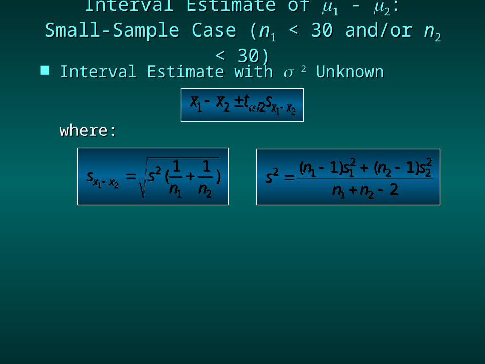
Interval Estimate of Interval Estimate of 11 - - 22::Small-Sample Case (Small-Sample Case (nn11 < 30 and/or < 30 and/or nn22 < <
30)30) Interval Estimate with Interval Estimate with 22 Unknown Unknown
where:where:x x t sx x1 2 2 1 2
/
s n s n sn n
2 1 12
2 22
1 2
1 12
( ) ( )s s
n nx x1 2
2
1 2
1 1 ( )
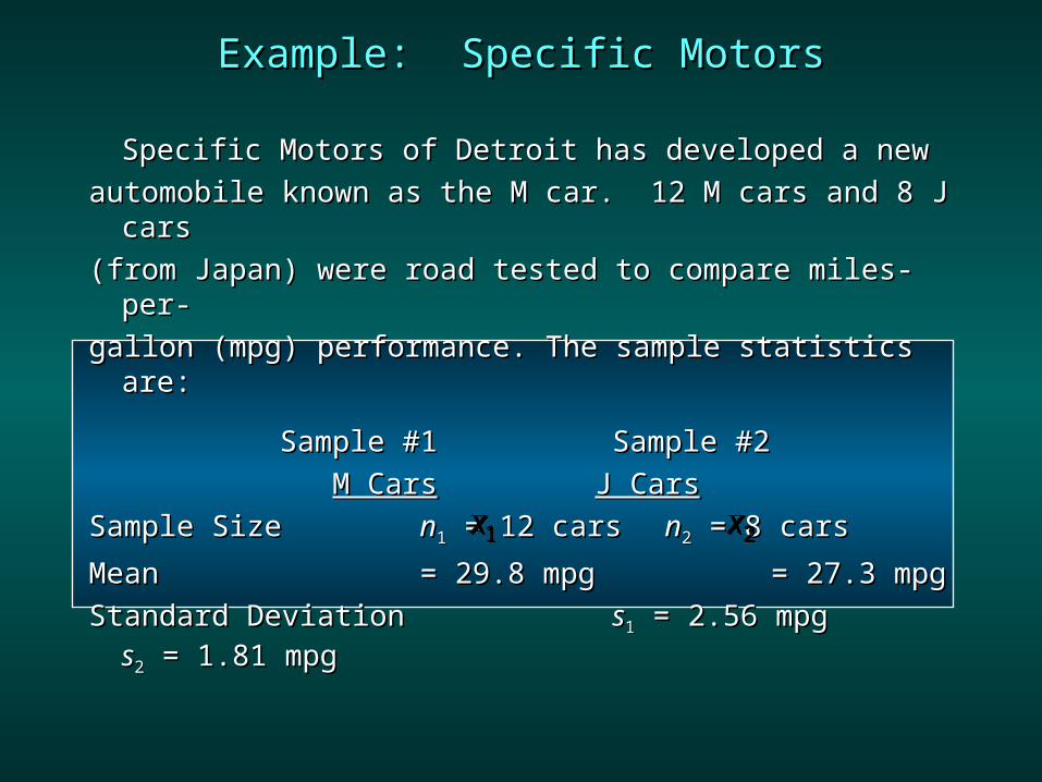
Example: Specific MotorsExample: Specific Motors
Specific Motors of Detroit has developed a newSpecific Motors of Detroit has developed a newautomobile known as the M car. 12 M cars and 8 J automobile known as the M car. 12 M cars and 8 J
carscars(from Japan) were road tested to compare miles-per-(from Japan) were road tested to compare miles-per-gallon (mpg) performance. The sample statistics are:gallon (mpg) performance. The sample statistics are:
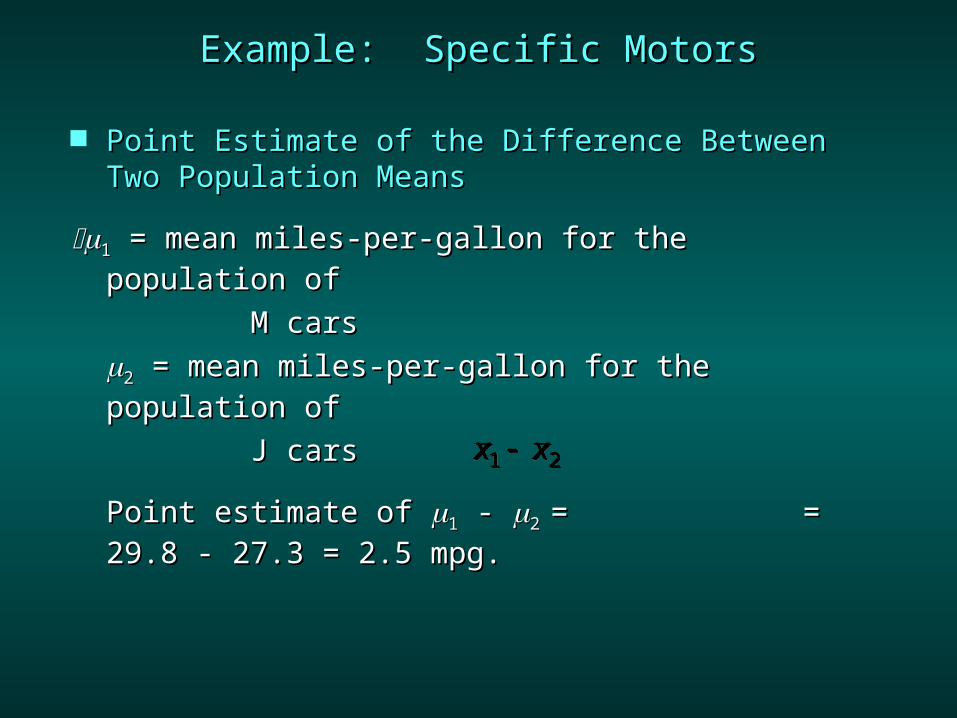
Point Estimate of the Difference Between Two Point Estimate of the Difference Between Two Population MeansPopulation Means
11 = mean miles-per-gallon for the population of = mean miles-per-gallon for the population of M carsM cars22 = mean miles-per-gallon for the population of = mean miles-per-gallon for the population of J carsJ carsPoint estimate of Point estimate of 11 - - 2 2 = = 29.8 - 27.3 = = 29.8 - 27.3 = 2.5 mpg.= 2.5 mpg.
x x1 2
Example: Specific MotorsExample: Specific Motors
95% Confidence Interval Estimate of the 95% Confidence Interval Estimate of the Difference Between Two Population Means: Difference Between Two Population Means: Small-Sample CaseSmall-Sample CaseWe will make the following assumptions:We will make the following assumptions:• The miles per gallon rating must be The miles per gallon rating must be
normally normally distributed for both the M car and the J car.distributed for both the M car and the J car.• The variance in the miles per gallon rating The variance in the miles per gallon rating
mustmust be the same for both the M car and the J be the same for both the M car and the J
car.car.
Example: Specific MotorsExample: Specific Motors
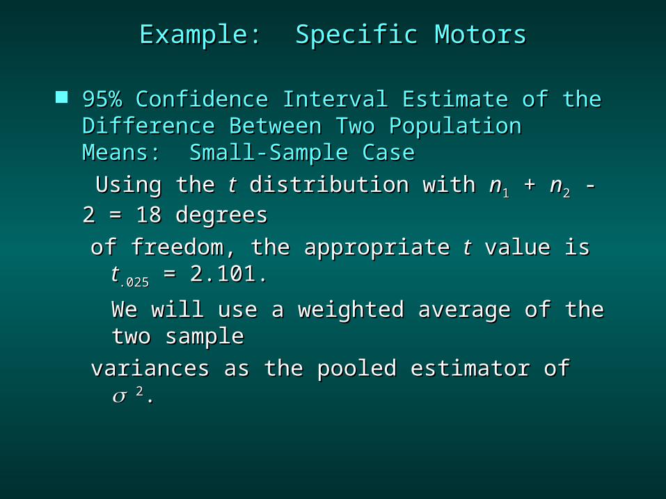
95% Confidence Interval Estimate of the 95% Confidence Interval Estimate of the Difference Between Two Population Means: Difference Between Two Population Means: Small-Sample CaseSmall-Sample Case Using the Using the tt distribution with distribution with nn11 + + nn22 - 2 = 18 - 2 = 18 degreesdegreesof freedom, the appropriate of freedom, the appropriate tt value is value is tt.025.025 = =
2.101.2.101.We will use a weighted average of the two We will use a weighted average of the two samplesample
variances as the pooled estimator of variances as the pooled estimator of 22..
Example: Specific MotorsExample: Specific Motors
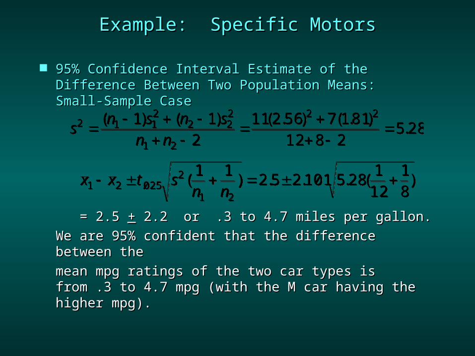
95% Confidence Interval Estimate of the Difference 95% Confidence Interval Estimate of the Difference Between Two Population Means: Small-Sample Between Two Population Means: Small-Sample CaseCase
= 2.5 = 2.5 ++ 2.2 or .3 to 4.7 miles per gallon. 2.2 or .3 to 4.7 miles per gallon.We are 95% confident that the difference between We are 95% confident that the difference between thethemean mpg ratings of the two car types is from .3 to mean mpg ratings of the two car types is from .3 to 4.7 mpg (with the M car having the higher mpg).4.7 mpg (with the M car having the higher mpg).
s n s n sn n
2 1 12
2 22
1 2
2 21 12
11 2 56 7 1 8112 8 2
5 28
( ) ( ) ( . ) ( . ) .
x x t sn n1 2 025
2
1 2
1 1 2 5 2 101 5 28 112
18
. ( ) . . . ( )
Example: Specific MotorsExample: Specific Motors
Hypothesis Tests About the Difference Hypothesis Tests About the Difference between the Means of Two Populations: between the Means of Two Populations:
Test StatisticTest Statistic Large-SampleLarge-Sample
Small-SampleSmall-Samplez x x
n n
( ) ( )1 2 1 2
12
1 22
2
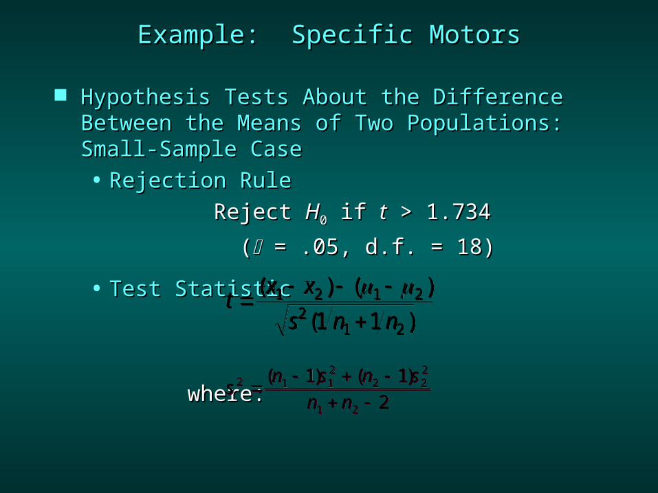
t x xs n n
( ) ( )
( )1 2 1 2
21 21 1
Hypothesis Tests About the Difference Hypothesis Tests About the Difference between the Means of Two Populations: between the Means of Two Populations: Large-Sample CaseLarge-Sample Case Par, Inc. is a Par, Inc. is a manufacturer of golf equipment and has manufacturer of golf equipment and has developed a new golf ball that has been developed a new golf ball that has been designed to provide “extra distance.” In a test designed to provide “extra distance.” In a test of driving distance using a mechanical driving of driving distance using a mechanical driving device, a sample of Par golf balls was device, a sample of Par golf balls was compared with a sample of golf balls made by compared with a sample of golf balls made by Rap, Ltd., a competitor. The sample statistics Rap, Ltd., a competitor. The sample statistics appear on the next slide.appear on the next slide.
Example: Par, Inc.Example: Par, Inc.
Example: Par, Inc.Example: Par, Inc.
Hypothesis Tests About the Difference Between Hypothesis Tests About the Difference Between the Means of Two Populations: Large-Sample the Means of Two Populations: Large-Sample CaseCase• Sample StatisticsSample Statistics
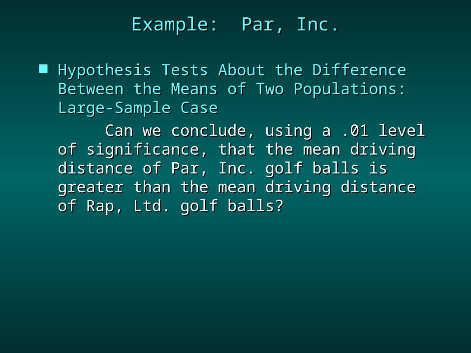
Hypothesis Tests About the Difference Hypothesis Tests About the Difference Between the Means of Two Populations: Between the Means of Two Populations: Large-Sample CaseLarge-Sample Case
Can we conclude, using a .01 level of Can we conclude, using a .01 level of significance, that the mean driving distance of significance, that the mean driving distance of Par, Inc. golf balls is greater than the mean Par, Inc. golf balls is greater than the mean driving distance of Rap, Ltd. golf balls?driving distance of Rap, Ltd. golf balls?
Example: Par, Inc.Example: Par, Inc.
Hypothesis Tests About the Difference Hypothesis Tests About the Difference Between the Means of Two Populations: Between the Means of Two Populations: Large-Sample CaseLarge-Sample Case
11 = mean distance for the population of Par, = mean distance for the population of Par, Inc.Inc.
golf ballsgolf balls22 = mean distance for the population of Rap, = mean distance for the population of Rap, Ltd.Ltd.
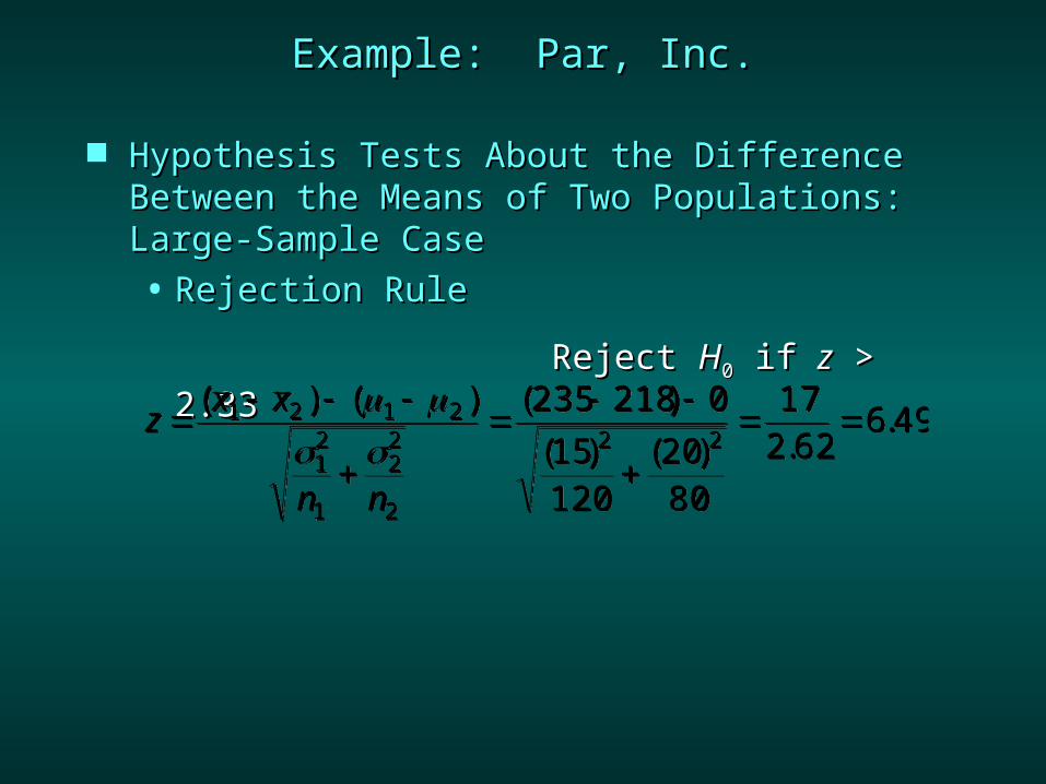
Hypothesis Tests About the Difference Hypothesis Tests About the Difference Between the Means of Two Populations: Between the Means of Two Populations: Large-Sample CaseLarge-Sample Case• Rejection RuleRejection Rule
Reject Reject HH00 if if zz > 2.33 > 2.33z x x
n n
( ) ( ) ( )
( ) ( ) ..1 2 1 2
12
1
22
2
2 2
235 218 015120
2080
172 62
6 49
Example: Par, Inc.Example: Par, Inc.
Hypothesis Tests About the Difference Hypothesis Tests About the Difference Between the Means of Two Populations: Between the Means of Two Populations: Large-Sample CaseLarge-Sample Case• ConclusionConclusion
Reject Reject HH00. We are at least 99% confident . We are at least 99% confident that the that the mean driving distance of Par, mean driving distance of Par,
Inc. golf balls is Inc. golf balls is greater than the mean greater than the mean driving distance of Rap, driving distance of Rap, Ltd. golf balls.Ltd. golf balls.
Example: Par, Inc.Example: Par, Inc.
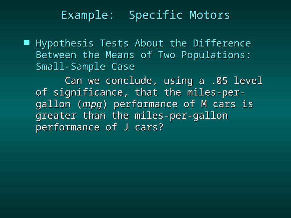
Hypothesis Tests About the Difference Hypothesis Tests About the Difference Between the Means of Two Populations: Between the Means of Two Populations: Small-Sample CaseSmall-Sample Case
Can we conclude, using a .05 level of Can we conclude, using a .05 level of significance, that the miles-per-gallon (significance, that the miles-per-gallon (mpgmpg) ) performance of M cars is greater than the performance of M cars is greater than the miles-per-gallon performance of J cars?miles-per-gallon performance of J cars?
Example: Specific MotorsExample: Specific Motors
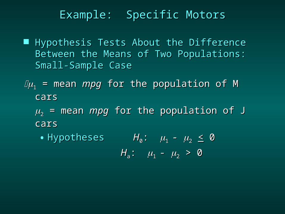
Hypothesis Tests About the Difference Hypothesis Tests About the Difference Between the Means of Two Populations: Between the Means of Two Populations: Small-Sample CaseSmall-Sample Case
11 = mean = mean mpgmpg for the population of M cars for the population of M cars22 = mean = mean mpgmpg for the population of J cars for the population of J cars• HypothesesHypotheses HH00: : 1 1 - - 22 << 0 0
HHaa: : 1 1 - - 22 > 0 > 0
Example: Specific MotorsExample: Specific Motors
Example: Specific MotorsExample: Specific Motors
Hypothesis Tests About the Difference Hypothesis Tests About the Difference Between the Means of Two Populations: Between the Means of Two Populations: Small-Sample CaseSmall-Sample Case• Rejection RuleRejection Rule
Inference About the Difference between Inference About the Difference between the Means of Two Populations: Matched the Means of Two Populations: Matched
SamplesSamples With a With a matched-sample designmatched-sample design each sampled each sampled
item provides a pair of data values.item provides a pair of data values. The matched-sample design can be referred to The matched-sample design can be referred to
as as blockingblocking.. This design often leads to a smaller sampling This design often leads to a smaller sampling
error than the independent-sample design error than the independent-sample design because variation between sampled items is because variation between sampled items is eliminated as a source of sampling error.eliminated as a source of sampling error.
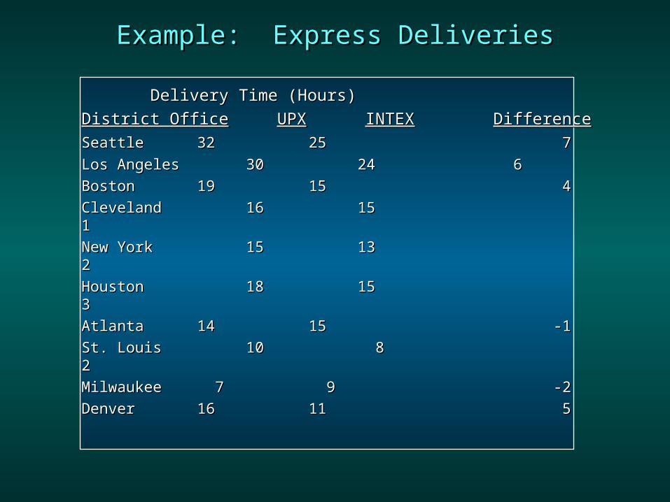
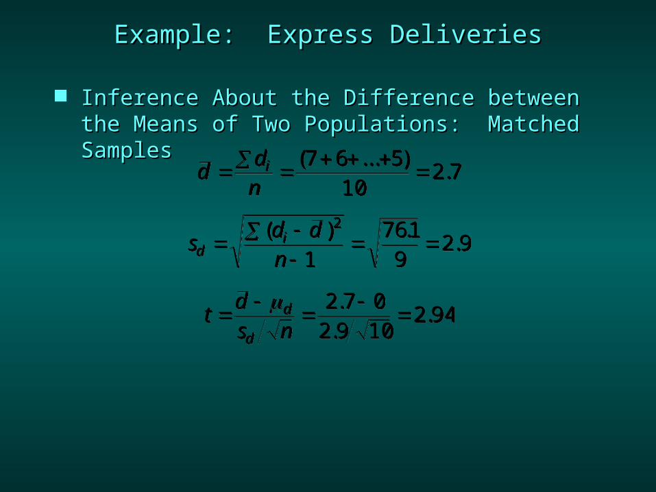
Inference About the Difference between the Inference About the Difference between the Means of Two Populations: Matched SamplesMeans of Two Populations: Matched Samples A Chicago-based firm has documents that must A Chicago-based firm has documents that must be quickly distributed to district offices be quickly distributed to district offices throughout the U.S. The firm must decide throughout the U.S. The firm must decide between two delivery services, UPX (United between two delivery services, UPX (United Parcel Express) and INTEX (International Parcel Express) and INTEX (International Express), to transport its documents. In testing Express), to transport its documents. In testing the delivery times of the two services, the firm the delivery times of the two services, the firm sent two reports to a random sample of ten sent two reports to a random sample of ten district offices with one report carried by UPX district offices with one report carried by UPX and the other report carried by INTEX.and the other report carried by INTEX.Do the data that follow indicate a difference in Do the data that follow indicate a difference in mean delivery times for the two services?mean delivery times for the two services?
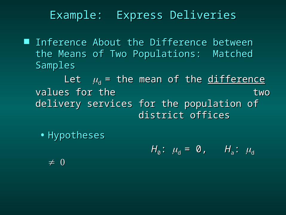
Inference About the Difference between the Inference About the Difference between the Means of Two Populations: Matched SamplesMeans of Two Populations: Matched Samples Let Let d d = the mean of the = the mean of the differencedifference values for values for the the two delivery services for the two delivery services for the population of population of district offices district offices• HypothesesHypotheses
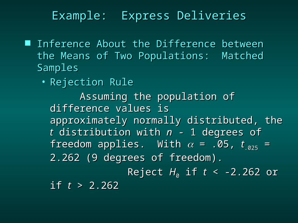
Inference About the Difference between the Inference About the Difference between the Means of Two Populations: Matched SamplesMeans of Two Populations: Matched Samples• Rejection RuleRejection Rule
Assuming the population of difference Assuming the population of difference values is approximately normally values is approximately normally distributed, the distributed, the tt distribution with distribution with nn - 1 - 1 degrees of freedom applies. With degrees of freedom applies. With = .05, = .05, tt.025.025 = 2.262 (9 degrees of freedom).= 2.262 (9 degrees of freedom).
Reject Reject HH00 if if tt < -2.262 or if < -2.262 or if tt > > 2.2622.262
Inference About the Difference between the Inference About the Difference between the Means of Two Populations: Matched SamplesMeans of Two Populations: Matched Samples
Inference About the Difference between the Inference About the Difference between the Means of Two Populations: Matched SamplesMeans of Two Populations: Matched Samples• ConclusionConclusion
Reject Reject HH00. . There is a significant difference between the There is a significant difference between the
mean delivery times for the two services. mean delivery times for the two services.
Introduction to Analysis of VarianceIntroduction to Analysis of Variance
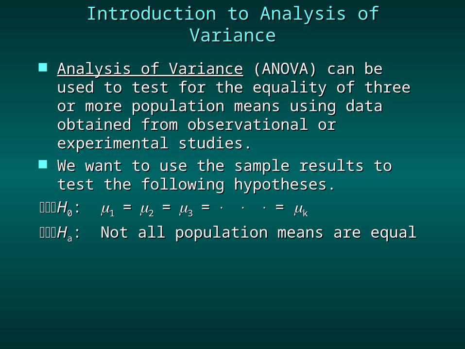
Analysis of VarianceAnalysis of Variance (ANOVA) can be used to (ANOVA) can be used to test for the equality of three or more test for the equality of three or more population means using data obtained from population means using data obtained from observational or experimental studies.observational or experimental studies.
We want to use the sample results to test the We want to use the sample results to test the following hypotheses.following hypotheses.
HH00: : 11==22==33==. . . . . . = = kk
HHaa: Not all population means are equal: Not all population means are equal
Introduction to Analysis of VarianceIntroduction to Analysis of Variance
If If HH00 is rejected, we cannot conclude that all is rejected, we cannot conclude that all population means are different.population means are different.
Rejecting Rejecting HH00 means that at least two means that at least two population means have different values.population means have different values.
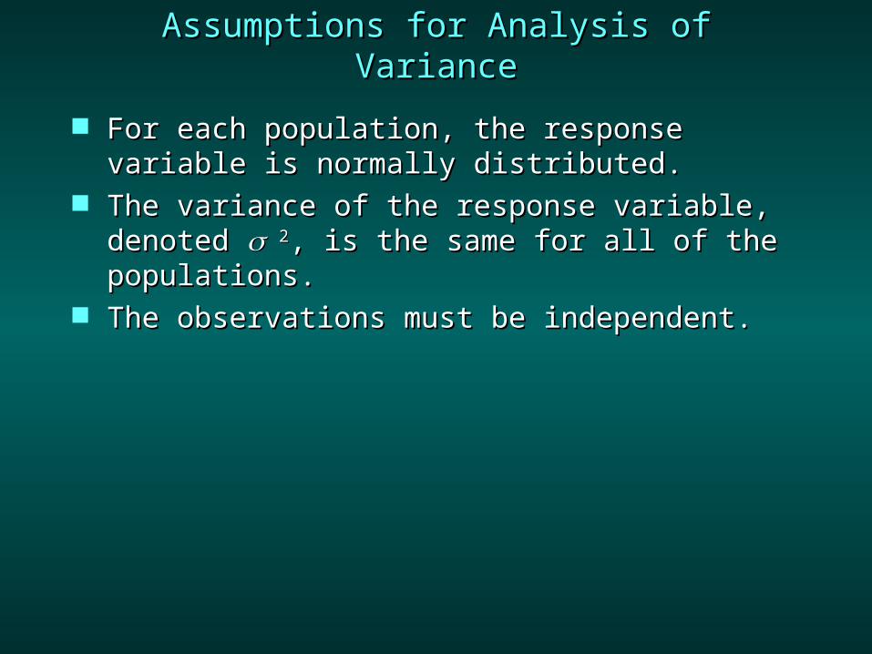
Assumptions for Analysis of VarianceAssumptions for Analysis of Variance
For each population, the response variable is For each population, the response variable is normally distributed.normally distributed.
The variance of the response variable, denoted The variance of the response variable, denoted 22, is the same for all of the populations., is the same for all of the populations.
The observations must be independent.The observations must be independent.
Analysis of Variance:Analysis of Variance:Testing for the Equality of Testing for the Equality of kk Population Population
MeansMeans Between-Treatments Estimate of Population Between-Treatments Estimate of Population
VarianceVariance Within-Treatments Estimate of Population Within-Treatments Estimate of Population
VarianceVariance Comparing the Variance Estimates: The Comparing the Variance Estimates: The F F Test Test The ANOVA TableThe ANOVA Table
Between-Treatments EstimateBetween-Treatments Estimateof Population Varianceof Population Variance
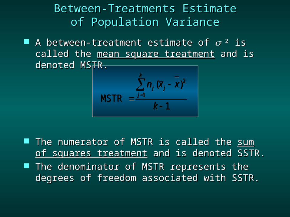
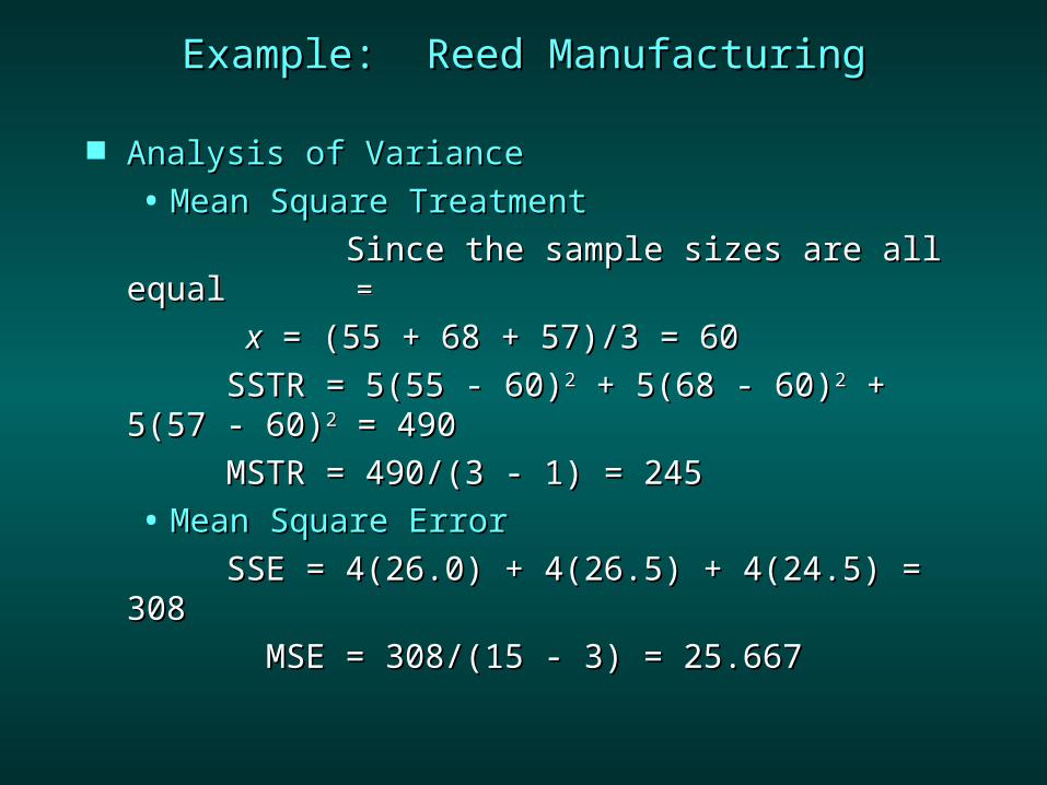
A between-treatment estimate of A between-treatment estimate of 2 2 is called is called the the mean square treatmentmean square treatment and is denoted and is denoted MSTR.MSTR.
The numerator of MSTR is called the The numerator of MSTR is called the sum of sum of squares treatmentsquares treatment and is denoted SSTR. and is denoted SSTR.
The denominator of MSTR represents the The denominator of MSTR represents the degrees of freedom associated with SSTR.degrees of freedom associated with SSTR.
1
)(MSTR 1
2
k
xxnk
jjj
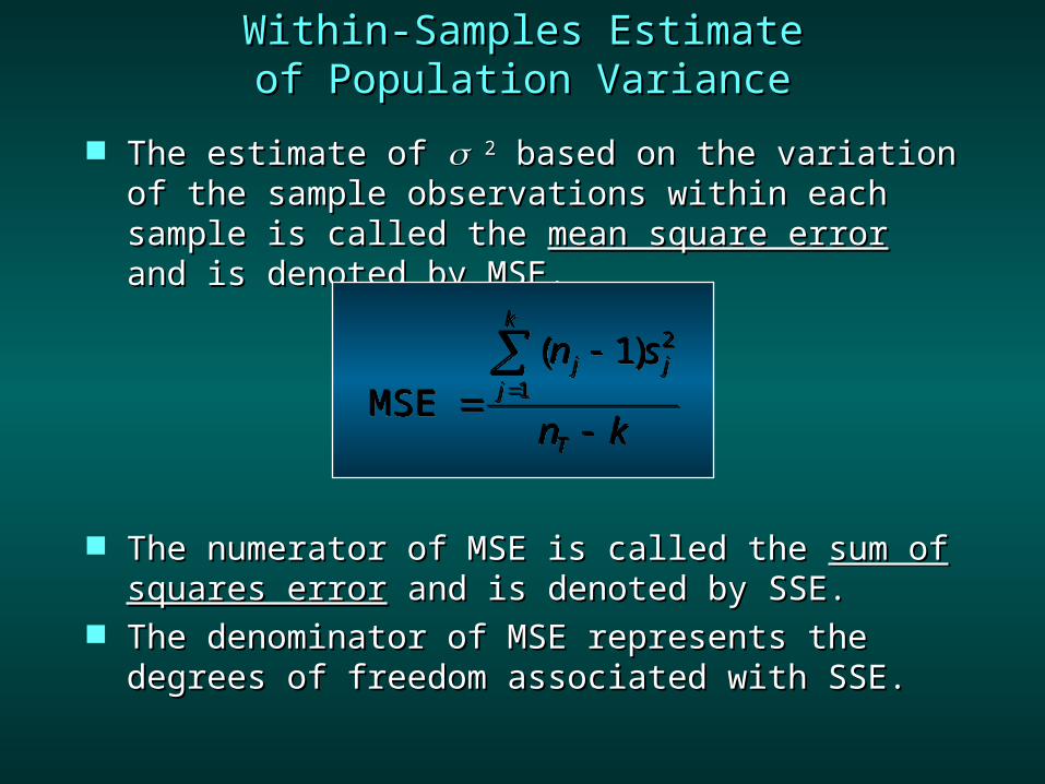
The estimate of The estimate of 22 based on the variation of the based on the variation of the sample observations within each sample is sample observations within each sample is called the called the mean square errormean square error and is denoted by and is denoted by MSE.MSE.
The numerator of MSE is called the The numerator of MSE is called the sum of sum of squares errorsquares error and is denoted by SSE. and is denoted by SSE.
The denominator of MSE represents the degrees The denominator of MSE represents the degrees of freedom associated with SSE.of freedom associated with SSE.
Within-Samples EstimateWithin-Samples Estimateof Population Varianceof Population Variance
kn
sn
T
k
jjj
1
2)1(MSE
Comparing the Variance Estimates: The Comparing the Variance Estimates: The FF TestTest
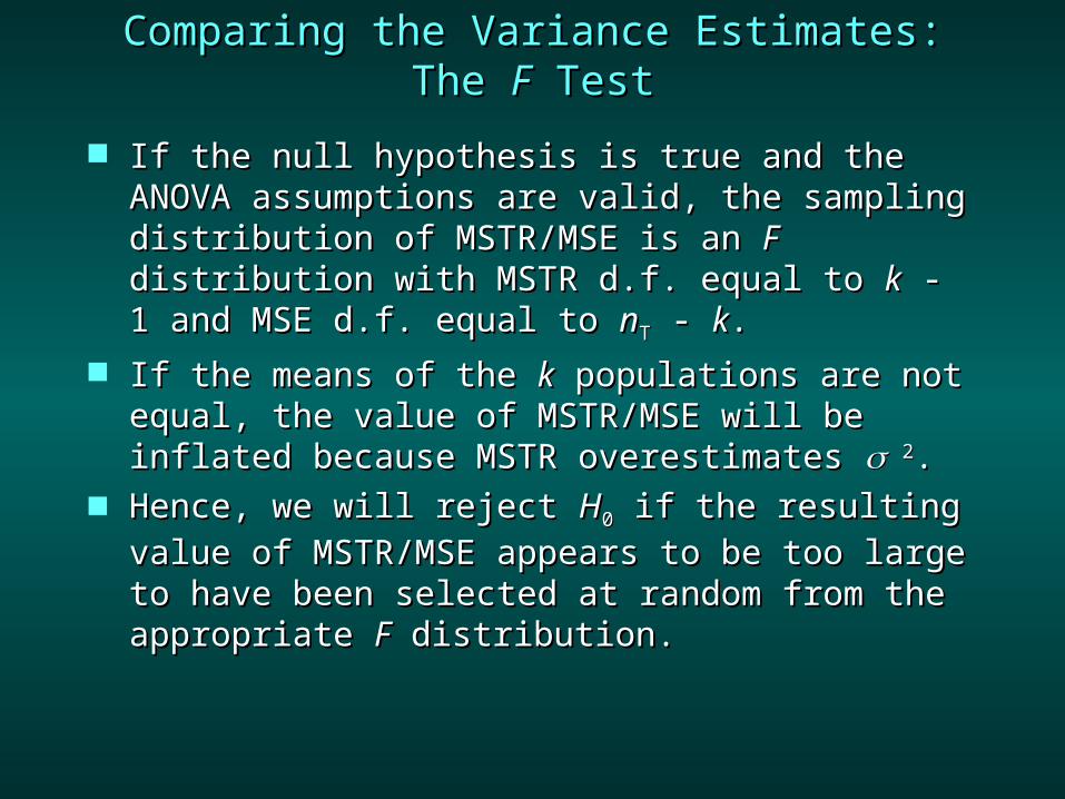
If the null hypothesis is true and the ANOVA If the null hypothesis is true and the ANOVA assumptions are valid, the sampling assumptions are valid, the sampling distribution of MSTR/MSE is an distribution of MSTR/MSE is an FF distribution distribution with MSTR d.f. equal to with MSTR d.f. equal to kk - 1 and MSE d.f. - 1 and MSE d.f. equal to equal to nnTT - - kk..
If the means of the If the means of the kk populations are not populations are not equal, the value of MSTR/MSE will be inflated equal, the value of MSTR/MSE will be inflated because MSTR overestimates because MSTR overestimates 22..
Hence, we will reject Hence, we will reject HH00 if the resulting value if the resulting value of MSTR/MSE appears to be too large to have of MSTR/MSE appears to be too large to have been selected at random from the appropriate been selected at random from the appropriate FF distribution. distribution.
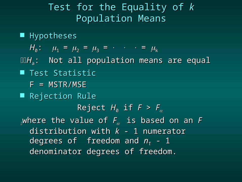
Test for the Equality of Test for the Equality of kk Population Population MeansMeans
HHaa: Not all population means are equal: Not all population means are equal Test StatisticTest Statistic
F = MSTR/MSEF = MSTR/MSE Rejection RuleRejection Rule
Reject Reject HH00 if if FF > > FF
where the value of where the value of FF is based on an is based on an FF distribution with distribution with kk - 1 numerator degrees of - 1 numerator degrees of freedom and freedom and nnTT - 1 denominator degrees of - 1 denominator degrees of freedom.freedom.
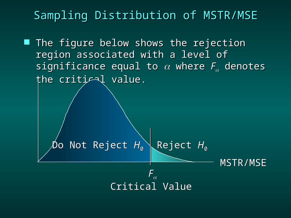
Sampling Distribution of MSTR/MSESampling Distribution of MSTR/MSE
The figure below shows the rejection region The figure below shows the rejection region associated with a level of significance equal to associated with a level of significance equal to where where FF denotes the critical value. denotes the critical value.
Do Not Reject H0 Reject H0
MSTR/MSE
Critical ValueF
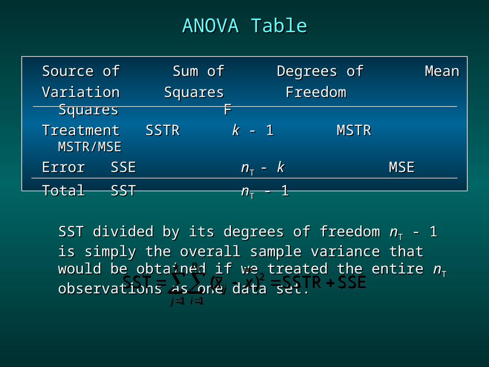
ANOVA TableANOVA Table
Source of Sum of Degrees of MeanSource of Sum of Degrees of MeanVariation Squares Freedom Squares Variation Squares Freedom Squares
FFTreatmentTreatment SSTRSSTR kk - 1 - 1 MSTR MSTR
MSTR/MSEMSTR/MSEErrorError SSESSE nnT T - - kk MSE MSETotalTotal SSTSST nnTT - 1 - 1
SST divided by its degrees of freedom SST divided by its degrees of freedom nnTT - 1 is - 1 is simply the overall sample variance that would be simply the overall sample variance that would be obtained if we treated the entire obtained if we treated the entire nnTT observations observations as one data set.as one data set.
Analysis of VarianceAnalysis of VarianceJ. R. Reed would like to know if the mean J. R. Reed would like to know if the mean
number of hours worked per week is the same number of hours worked per week is the same for the department managers at her three for the department managers at her three manufacturing plants (Buffalo, Pittsburgh, and manufacturing plants (Buffalo, Pittsburgh, and Detroit). Detroit).
A simple random sample of 5 managers A simple random sample of 5 managers from each of the three plants was taken and from each of the three plants was taken and the number of hours worked by each manager the number of hours worked by each manager for the previous week is shown on the next for the previous week is shown on the next slide.slide.
Analysis of VarianceAnalysis of Variance Plant 1Plant 1 Plant 2 Plant 2 Plant 3Plant 3
Analysis of VarianceAnalysis of Variance• HypothesesHypotheses
HH00: : 11==22==33
HHaa: Not all the means are equal: Not all the means are equal where: where:
1 1 = mean number of hours worked per = mean number of hours worked per week by the managers at Plant 1 week by the managers at Plant 1 2 2 = mean number of hours worked per = mean number of hours worked per week by the managers at Plant 2week by the managers at Plant 2
3 3 = mean number of hours worked per = mean number of hours worked per week by the managers at Plant 3 week by the managers at Plant 3
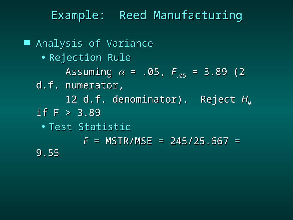
Analysis of VarianceAnalysis of Variance• FF - Test - Test
If If HH00 is true, the ratio MSTR/MSE should be is true, the ratio MSTR/MSE should be nearnear 1 since both MSTR and MSE are estimating 1 since both MSTR and MSE are estimating 22. If. If HHa a is true, the ratio should be significantly is true, the ratio should be significantly largerlarger than 1 since MSTR tends to overestimate than 1 since MSTR tends to overestimate 22..
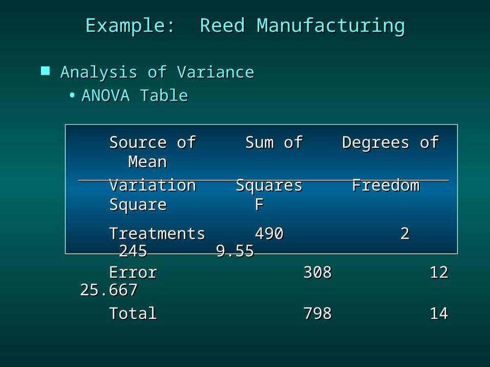
Analysis of VarianceAnalysis of Variance• ANOVA TableANOVA Table
Source of Sum of Degrees of MeanSource of Sum of Degrees of Mean Variation Squares Freedom Square Variation Squares Freedom Square F F Treatments Treatments 490490 2 2 245 245 9.55 9.55 ErrorError 308308 12 12 25.667 25.667 TotalTotal 798 798 1414
Analysis of VarianceAnalysis of Variance• ConclusionConclusion
FF = 9.55 > = 9.55 > FF.05.05 = 3.89, so we reject = 3.89, so we reject HH00. . The meanThe mean number of hours worked per week by number of hours worked per week by departmentdepartment managers is not the same at each plant.managers is not the same at each plant.