58
Seoul National University Tilted and Oblique Photographs Chapter 10. Tilted and Oblique Photographs
Seoul National University
Tilted and Oblique Photographs
Chapter 10. Tilted and Oblique Photographs
Unavoidable aircraft tilts cause photographs to be exposed with the camera axis tilted
slightly from vertical, and the resulting pictures are called tilted photographs
In some cases, aerial photography is purposely angled away from vertical
⇨ These types of images are classified as high oblique if the photograph contains the
horizon, and low oblique otherwise
Terrestrial photos are almost always taken from an oblique pose
⇨ Horizontal terrestrial photos are obtained if the camera axis is horizontal when the
exposure is made
Six independent parameters called the elements of exterior orientation (sometimes
called EOPs) express the spatial position and angular orientation of a photograph
⇨ The spatial position is normally given by 𝑋𝐿 , 𝑌𝐿 , and 𝑍𝐿, the three dimensional
coordinates of the exposure station in a ground coordinate system
⇨ 𝑍𝐿 is called 𝐻, the height above datum
Angular orientation is the amount and direction of tilt in the photo
10-1. Introduction
Seoul National University
Tilted and Oblique Photographs
Unavoidable aircraft tilts cause photographs to be exposed with the camera axis tilted
slightly from vertical, and the resulting pictures are called tilted photographs
In some cases, aerial photography is purposely angled away from vertical
⇨ These types of images are classified as high oblique if the photograph contains the
horizon, and low oblique otherwise
Terrestrial photos are almost always taken from an oblique pose
⇨ Horizontal terrestrial photos are obtained if the camera axis is horizontal when the
exposure is made
10-1. Introduction
Seoul National University
Tilted and Oblique Photographs
In this book, two different systems are described: (1) the tilt-swing-azimuth (𝒕 − 𝒔 − 𝜶) system (2) the omega-phi-kappa (𝝎−𝝓− 𝜿) system
The omega-phi-kappa system possesses certain computational advantages over
the tilt-swing-azimuth system and is therefore more widely used
The tilt-swing-azimuth system, however, is more easily understood and shall therefore be considered first
Perspective can be defined as how something is visually perceived under varying
circumstances
Some important properties of a perspective projection are that straight lines are preserved
and projected lines that are parallel in object space intersect when projected onto the
image plane
More specifically, horizontal parallel lines intersect at the horizon, and vertical lines
intersect at either the zenith or nadir in an image
⇨ The locations at which these lines intersect on images are called vanishing points
10-2. Point Perspective
Seoul National University
Tilted and Oblique Photographs
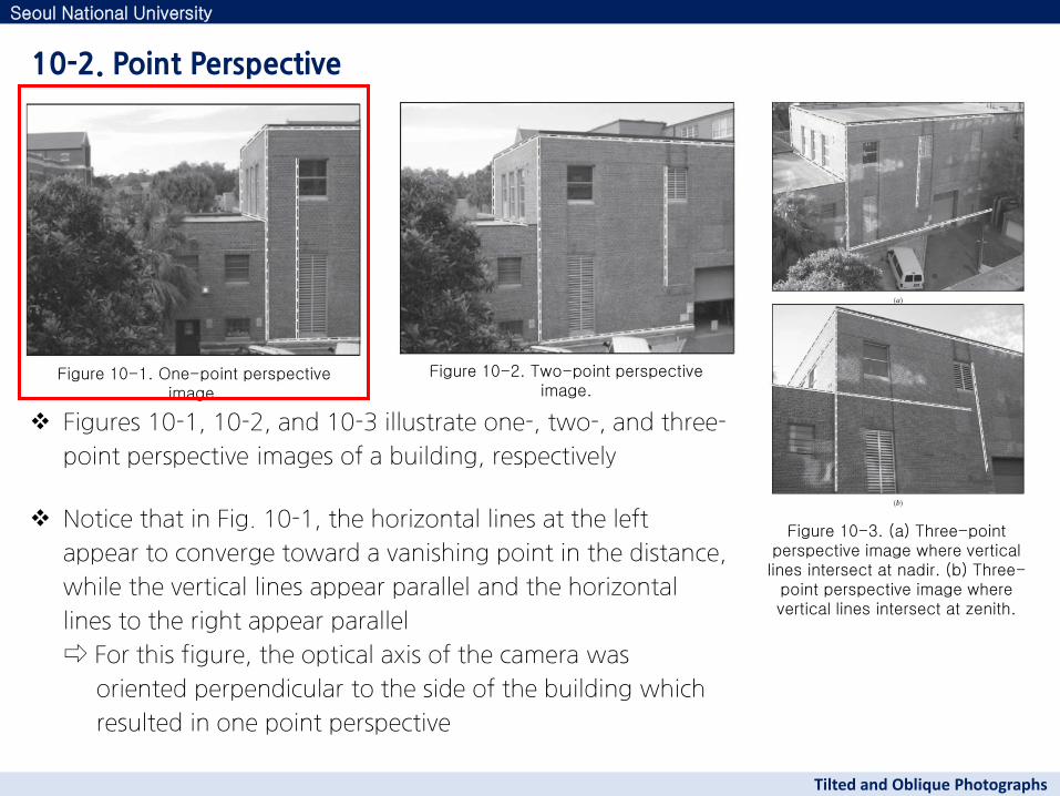
Figures 10-1, 10-2, and 10-3 illustrate one-, two-, and three-
point perspective images of a building, respectively
Notice that in Fig. 10-1, the horizontal lines at the left
appear to converge toward a vanishing point in the distance,
while the vertical lines appear parallel and the horizontal
lines to the right appear parallel
⇨ For this figure, the optical axis of the camera was
oriented perpendicular to the side of the building which
resulted in one point perspective
10-2. Point Perspective
Seoul National University
Tilted and Oblique Photographs
Figure 10-2. Two-point perspective image.
Figure 10-3. (a) Three-point perspective image where vertical lines intersect at nadir. (b) Three-
point perspective image where vertical lines intersect at zenith.
Figure 10-1. One-point perspective image.
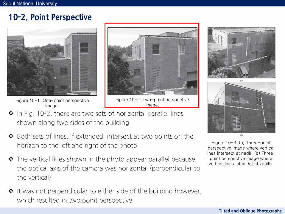
In Fig. 10-2, there are two sets of horizontal parallel lines
shown along two sides of the building
Both sets of lines, if extended, intersect at two points on the
horizon to the left and right of the photo
The vertical lines shown in the photo appear parallel because
the optical axis of the camera was horizontal (perpendicular to
the vertical)
It was not perpendicular to either side of the building however,
which resulted in two point perspective
10-2. Point Perspective
Seoul National University
Tilted and Oblique Photographs
Figure 10-1. One-point perspective image.
Figure 10-2. Two-point perspective image.
Figure 10-3. (a) Three-point perspective image where vertical lines intersect at nadir. (b) Three-
point perspective image where vertical lines intersect at zenith.
10-2. Point Perspective
Seoul National University
Tilted and Oblique Photographs
Figure 10-2. Two-point perspective image.
Figure 10-3. (a) Three-point perspective image where vertical lines intersect at nadir. (b) Three-
point perspective image where vertical lines intersect at zenith.
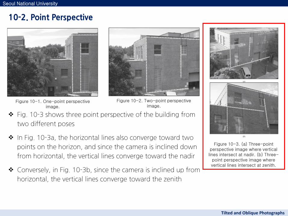
Fig. 10-3 shows three point perspective of the building from
two different poses
In Fig. 10-3a, the horizontal lines also converge toward two
points on the horizon, and since the camera is inclined down
from horizontal, the vertical lines converge toward the nadir
Conversely, in Fig. 10-3b, since the camera is inclined up from
horizontal, the vertical lines converge toward the zenith
Figure 10-1. One-point perspective image.
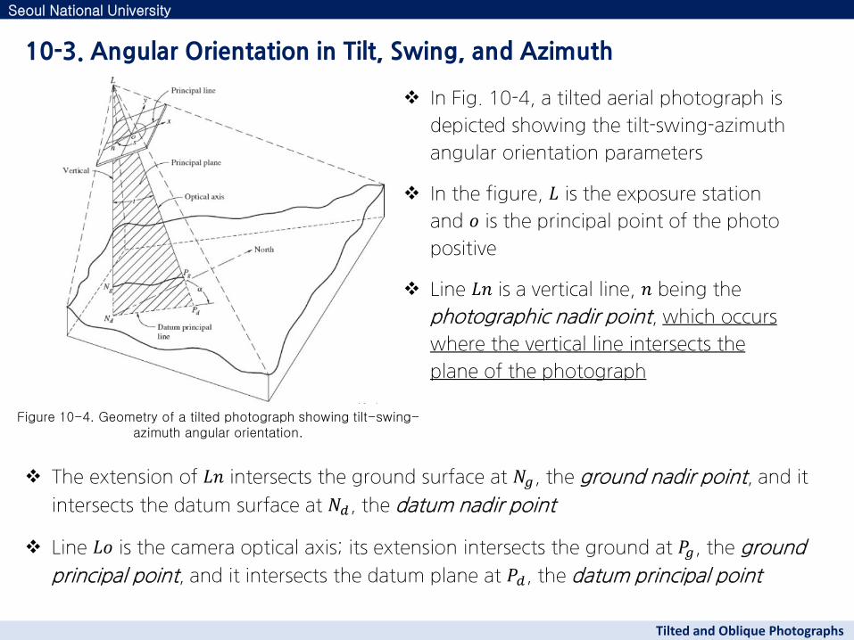
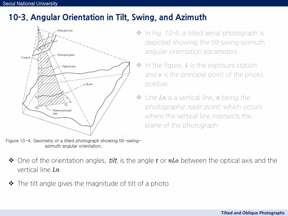
In Fig. 10-4, a tilted aerial photograph is
depicted showing the tilt-swing-azimuth
angular orientation parameters
In the figure, 𝐿 is the exposure station
and 𝑜 is the principal point of the photo
positive
Line 𝐿𝑛 is a vertical line, 𝑛 being the
photographic nadir point, which occurs
where the vertical line intersects the
plane of the photograph
10-3. Angular Orientation in Tilt, Swing, and Azimuth
Seoul National University
Tilted and Oblique Photographs
Figure 10-4. Geometry of a tilted photograph showing tilt-swing-azimuth angular orientation.
The extension of 𝐿𝑛 intersects the ground surface at 𝑁𝑔, the ground nadir point, and it
intersects the datum surface at 𝑁𝑑, the datum nadir point
Line 𝐿𝑜 is the camera optical axis; its extension intersects the ground at 𝑃𝑔, the ground
principal point, and it intersects the datum plane at 𝑃𝑑, the datum principal point
10-3. Angular Orientation in Tilt, Swing, and Azimuth
Seoul National University
Tilted and Oblique Photographs
Figure 10-4. Geometry of a tilted photograph showing tilt-swing-azimuth angular orientation.
One of the orientation angles, tilt, is the angle 𝑡 or 𝑛𝐿𝑜 between the optical axis and the
vertical line 𝐿𝑛
The tilt angle gives the magnitude of tilt of a photo
In Fig. 10-4, a tilted aerial photograph is
depicted showing the tilt-swing-azimuth
angular orientation parameters
In the figure, 𝐿 is the exposure station
and 𝑜 is the principal point of the photo
positive
Line 𝐿𝑛 is a vertical line, 𝑛 being the
photographic nadir point, which occurs
where the vertical line intersects the
plane of the photograph
10-3. Angular Orientation in Tilt, Swing, and Azimuth
Seoul National University
Tilted and Oblique Photographs
Figure 10-4. Geometry of a tilted photograph showing tilt-swing-azimuth angular orientation.
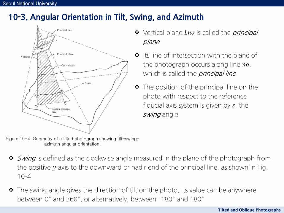
Vertical plane 𝐿𝑛𝑜 is called the principal
plane
Its line of intersection with the plane of
the photograph occurs along line 𝑛𝑜,
which is called the principal line
The position of the principal line on the
photo with respect to the reference
fiducial axis system is given by 𝑠, the
swing angle
Swing is defined as the clockwise angle measured in the plane of the photograph from
the positive 𝑦 axis to the downward or nadir end of the principal line, as shown in Fig.
10-4
The swing angle gives the direction of tilt on the photo. Its value can be anywhere
between 0° and 360°, or alternatively, between –180° and 180°
10-3. Angular Orientation in Tilt, Swing, and Azimuth
Seoul National University
Tilted and Oblique Photographs
Figure 10-4. Geometry of a tilted photograph showing tilt-swing-azimuth angular orientation.
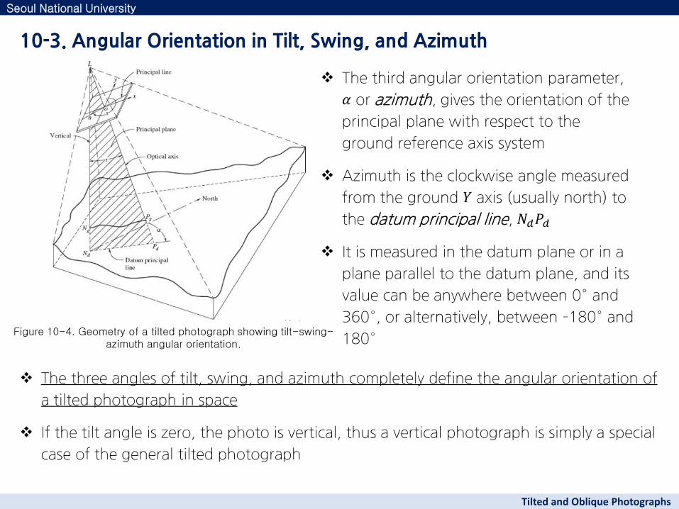
The third angular orientation parameter,
𝛼 or azimuth, gives the orientation of the
principal plane with respect to the
ground reference axis system
Azimuth is the clockwise angle measured
from the ground 𝑌 axis (usually north) to
the datum principal line, 𝑁𝑑𝑃𝑑
It is measured in the datum plane or in a
plane parallel to the datum plane, and its
value can be anywhere between 0° and
360°, or alternatively, between –180° and
180°
The three angles of tilt, swing, and azimuth completely define the angular orientation of
a tilted photograph in space
If the tilt angle is zero, the photo is vertical, thus a vertical photograph is simply a special
case of the general tilted photograph
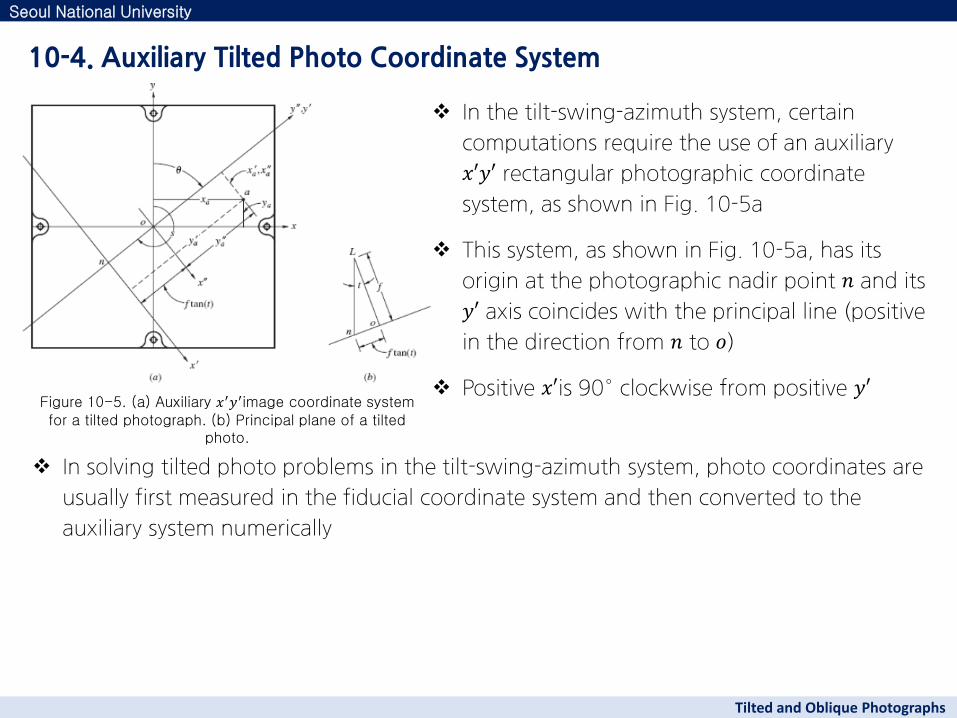
Figure 10-5. (a) Auxiliary 𝑥′𝑦′image coordinate system for a tilted photograph. (b) Principal plane of a tilted
photo.
In solving tilted photo problems in the tilt-swing-azimuth system, photo coordinates are
usually first measured in the fiducial coordinate system and then converted to the
auxiliary system numerically
10-4. Auxiliary Tilted Photo Coordinate System
Seoul National University
Tilted and Oblique Photographs
In the tilt-swing-azimuth system, certain
computations require the use of an auxiliary
𝑥′𝑦′ rectangular photographic coordinate
system, as shown in Fig. 10-5a
This system, as shown in Fig. 10-5a, has its
origin at the photographic nadir point 𝑛 and its
𝑦′ axis coincides with the principal line (positive
in the direction from 𝑛 to 𝑜)
Positive 𝑥′is 90° clockwise from positive 𝑦′
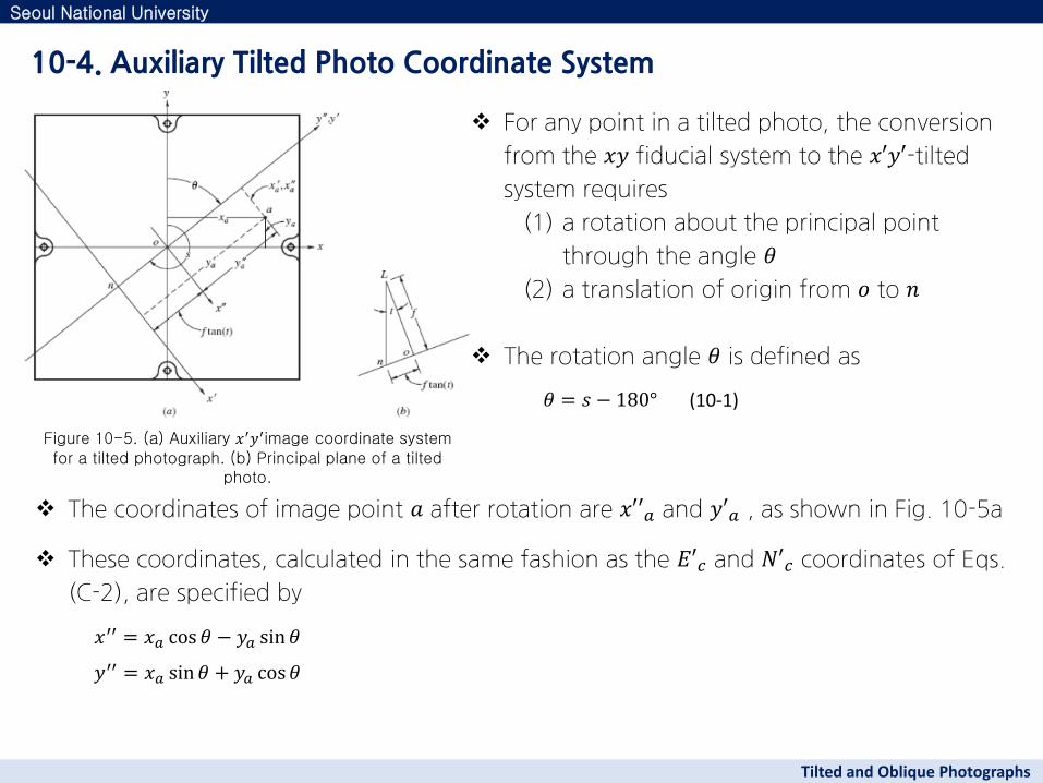
Figure 10-5. (a) Auxiliary 𝑥′𝑦′image coordinate system for a tilted photograph. (b) Principal plane of a tilted
photo.
The coordinates of image point 𝑎 after rotation are 𝑥′′𝑎 and 𝑦′𝑎 , as shown in Fig. 10-5a
These coordinates, calculated in the same fashion as the 𝐸′𝑐 and 𝑁′𝑐 coordinates of Eqs.
(C-2), are specified by
10-4. Auxiliary Tilted Photo Coordinate System
Seoul National University
Tilted and Oblique Photographs
For any point in a tilted photo, the conversion
from the 𝑥𝑦 fiducial system to the 𝑥′𝑦′-tilted
system requires
(1) a rotation about the principal point
through the angle 𝜃
(2) a translation of origin from 𝑜 to 𝑛
The rotation angle 𝜃 is defined as
𝜃 = 𝑠 − 180° (10-1)
𝑥′′ = 𝑥𝑎 cos 𝜃 − 𝑦𝑎 sin 𝜃
𝑦′′ = 𝑥𝑎 sin 𝜃 + 𝑦𝑎 cos𝜃
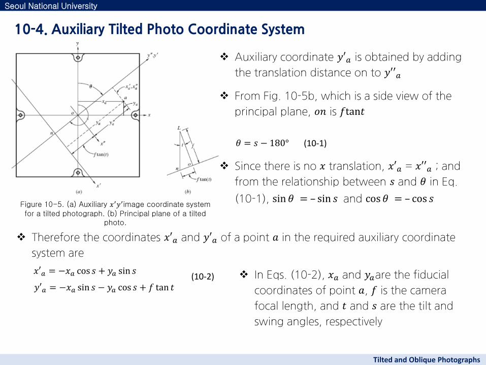
Figure 10-5. (a) Auxiliary 𝑥′𝑦′image coordinate system for a tilted photograph. (b) Principal plane of a tilted
photo.
Therefore the coordinates 𝑥′𝑎 and 𝑦′𝑎 of a point 𝑎 in the required auxiliary coordinate
system are
10-4. Auxiliary Tilted Photo Coordinate System
Seoul National University
Tilted and Oblique Photographs
Auxiliary coordinate 𝑦′𝑎 is obtained by adding
the translation distance on to 𝑦′′𝑎
From Fig. 10-5b, which is a side view of the
principal plane, 𝑜𝑛 is 𝑓tan𝑡
Since there is no 𝑥 translation, 𝑥′𝑎 = 𝑥′′𝑎 ; and
from the relationship between 𝑠 and 𝜃 in Eq.
(10-1), sin𝜃 =– sin𝑠 and cos𝜃 =– cos𝑠
𝜃 = 𝑠 − 180° (10-1)
𝑥′𝑎 = −𝑥𝑎 cos 𝑠 + 𝑦𝑎 sin 𝑠
𝑦′𝑎 = −𝑥𝑎 sin 𝑠 − 𝑦𝑎 cos 𝑠 + 𝑓 tan 𝑡 (10-2) In Eqs. (10-2), 𝑥𝑎 and 𝑦𝑎are the fiducial
coordinates of point 𝑎, 𝑓 is the camera
focal length, and 𝑡 and 𝑠 are the tilt and
swing angles, respectively
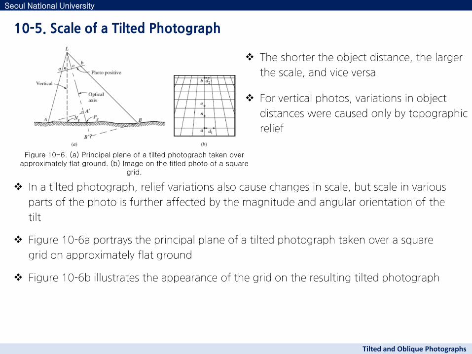
The shorter the object distance, the larger
the scale, and vice versa
For vertical photos, variations in object
distances were caused only by topographic
relief
In a tilted photograph, relief variations also cause changes in scale, but scale in various
parts of the photo is further affected by the magnitude and angular orientation of the
tilt
Figure 10-6a portrays the principal plane of a tilted photograph taken over a square
grid on approximately flat ground
Figure 10-6b illustrates the appearance of the grid on the resulting tilted photograph
10-5. Scale of a Tilted Photograph
Seoul National University
Tilted and Oblique Photographs
Figure 10-6. (a) Principal plane of a tilted photograph taken over approximately flat ground. (b) Image on the titled photo of a square
grid.
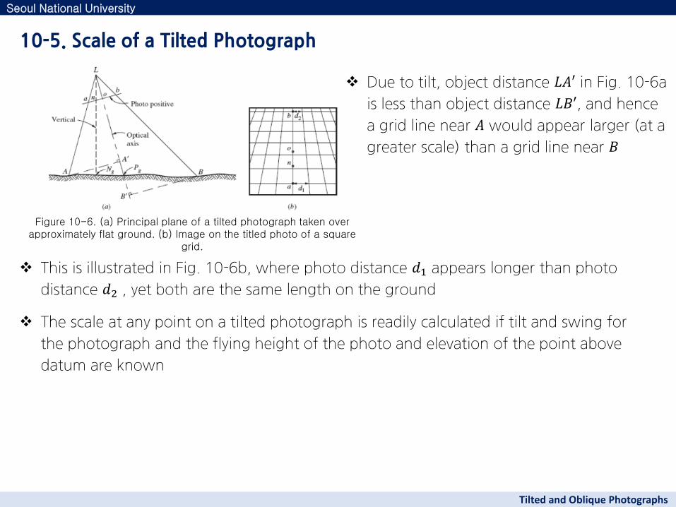
Due to tilt, object distance 𝐿𝐴′ in Fig. 10-6a
is less than object distance 𝐿𝐵′, and hence
a grid line near 𝐴 would appear larger (at a
greater scale) than a grid line near 𝐵
This is illustrated in Fig. 10-6b, where photo distance 𝑑1 appears longer than photo
distance 𝑑2 , yet both are the same length on the ground
The scale at any point on a tilted photograph is readily calculated if tilt and swing for
the photograph and the flying height of the photo and elevation of the point above
datum are known
10-5. Scale of a Tilted Photograph
Seoul National University
Tilted and Oblique Photographs
Figure 10-6. (a) Principal plane of a tilted photograph taken over approximately flat ground. (b) Image on the titled photo of a square
grid.

Figure 10-7 illustrates a tilted photo taken from a flying
height 𝐻 above datum; 𝐿𝑜 is the camera focal length
The image of object point 𝐴 appears at 𝑎 on the tilted
photo, and its coordinates in the auxiliary tilted photo
coordinate system are 𝑥′𝑎 and 𝑦′𝑎
The elevation of object point 𝐴 above datum is 𝐴
Object plane 𝐴𝐴′𝐾𝐾′ is a horizontal plane constructed at
𝑎 distance 𝐴 above datum
Image plane 𝑎𝑎′𝑘𝑘′ is also constructed horizontally
The scale relationship between the two parallel planes is the scale of the tilted
photograph at point 𝑎 because the image plane contains image point 𝑎 and the object
plane contains object point 𝐴
10-5. Scale of a Tilted Photograph
Seoul National University
Tilted and Oblique Photographs
Figure 10-7. Scale of a tilted photograph.
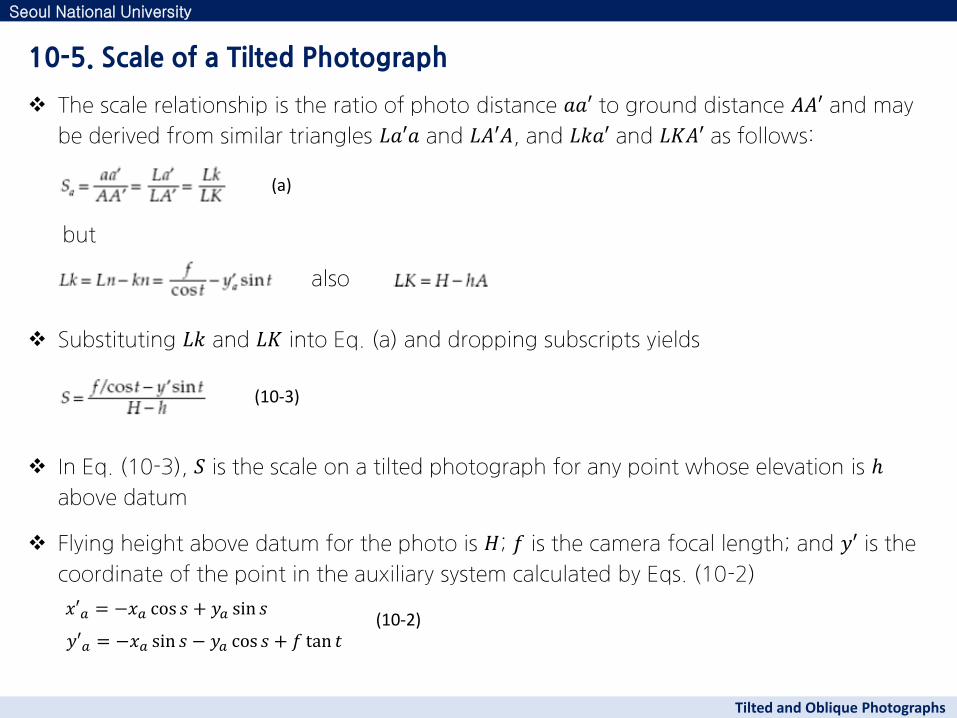
The scale relationship is the ratio of photo distance 𝑎𝑎′ to ground distance 𝐴𝐴′ and may
be derived from similar triangles 𝐿𝑎′𝑎 and 𝐿𝐴′𝐴, and 𝐿𝑘𝑎′ and 𝐿𝐾𝐴′ as follows:
but
also
Substituting 𝐿𝑘 and 𝐿𝐾 into Eq. (a) and dropping subscripts yields
10-5. Scale of a Tilted Photograph
Seoul National University
Tilted and Oblique Photographs
(a)
(10-3)
In Eq. (10-3), 𝑆 is the scale on a tilted photograph for any point whose elevation is
above datum
Flying height above datum for the photo is 𝐻; 𝑓 is the camera focal length; and 𝑦′ is the
coordinate of the point in the auxiliary system calculated by Eqs. (10-2)
𝑥′𝑎 = −𝑥𝑎 cos 𝑠 + 𝑦𝑎 sin 𝑠
𝑦′𝑎 = −𝑥𝑎 sin 𝑠 − 𝑦𝑎 cos 𝑠 + 𝑓 tan 𝑡 (10-2)
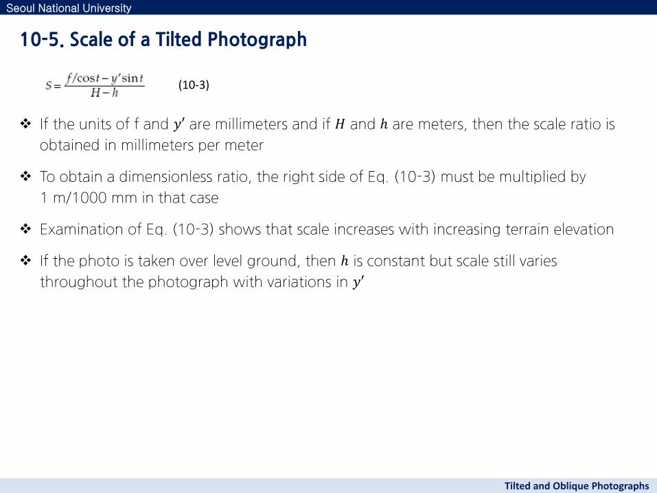
If the units of f and 𝑦′ are millimeters and if 𝐻 and are meters, then the scale ratio is
obtained in millimeters per meter
To obtain a dimensionless ratio, the right side of Eq. (10-3) must be multiplied by
1 m/1000 mm in that case
Examination of Eq. (10-3) shows that scale increases with increasing terrain elevation
If the photo is taken over level ground, then is constant but scale still varies
throughout the photograph with variations in 𝑦′
10-5. Scale of a Tilted Photograph
Seoul National University
Tilted and Oblique Photographs
(10-3)
Image displacements on tilted photographs caused by topographic relief occur much the
same as they do on vertical photos, except that relief displacements on tilted photographs
occur along radial lines from the nadir point
Relief displacements on a truly vertical photograph are also radial from the nadir point,
but in that special case the nadir point coincides with the principal point
On a tilted photograph, image displacements due to relief vary in magnitude depending
upon flying height, height of object, amount of tilt, and location of the image in the
photograph
Relief displacement is zero for images at the nadir point and increases with increased
radial distances from the nadir
Tilted photos are those that were intended to be vertical, but contain small unavoidable
amounts of tilt
In practice, tilted photos are therefore so nearly vertical that their nadir points are
generally very close to their principal points
10-6. Relief Displacement on a Tilted Photograph
Seoul National University
Tilted and Oblique Photographs
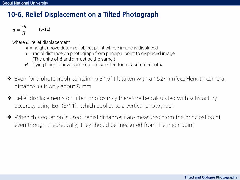
Even for a photograph containing 3° of tilt taken with a 152-mmfocal-length camera,
distance 𝑜𝑛 is only about 8 mm
Relief displacements on tilted photos may therefore be calculated with satisfactory
accuracy using Eq. (6-11), which applies to a vertical photograph
When this equation is used, radial distances r are measured from the principal point,
even though theoretically, they should be measured from the nadir point
10-6. Relief Displacement on a Tilted Photograph
Seoul National University
Tilted and Oblique Photographs
𝑑 =𝑟
𝐻 (6-11)
where 𝑑=relief displacement = height above datum of object point whose image is displaced 𝑟 = radial distance on photograph from principal point to displaced image (The units of 𝑑 and 𝑟 must be the same.) 𝐻 = flying height above same datum selected for measurement of
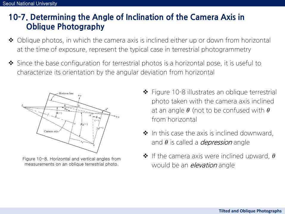
Oblique photos, in which the camera axis is inclined either up or down from horizontal
at the time of exposure, represent the typical case in terrestrial photogrammetry
Since the base configuration for terrestrial photos is a horizontal pose, it is useful to
characterize its orientation by the angular deviation from horizontal
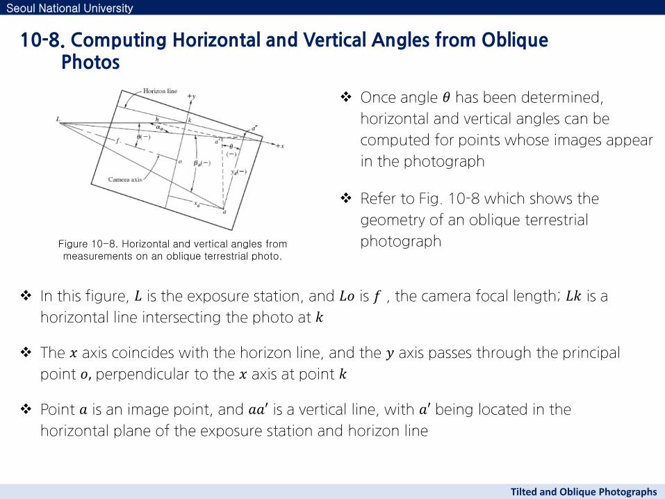
Figure 10-8 illustrates an oblique terrestrial
photo taken with the camera axis inclined
at an angle 𝜃 (not to be confused with 𝜃
from horizontal
In this case the axis is inclined downward,
and 𝜃 is called a depression angle
If the camera axis were inclined upward, 𝜃
would be an elevation angle
10-7. Determining the Angle of Inclination of the Camera Axis in Oblique Photography
Seoul National University
Tilted and Oblique Photographs
Figure 10-8. Horizontal and vertical angles from measurements on an oblique terrestrial photo.
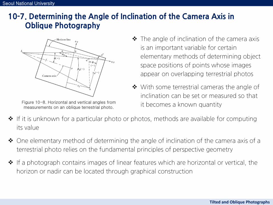
The angle of inclination of the camera axis
is an important variable for certain
elementary methods of determining object
space positions of points whose images
appear on overlapping terrestrial photos
With some terrestrial cameras the angle of
inclination can be set or measured so that
it becomes a known quantity
If it is unknown for a particular photo or photos, methods are available for computing
its value
One elementary method of determining the angle of inclination of the camera axis of a
terrestrial photo relies on the fundamental principles of perspective geometry
If a photograph contains images of linear features which are horizontal or vertical, the
horizon or nadir can be located through graphical construction
10-7. Determining the Angle of Inclination of the Camera Axis in Oblique Photography
Seoul National University
Tilted and Oblique Photographs
Figure 10-8. Horizontal and vertical angles from measurements on an oblique terrestrial photo.
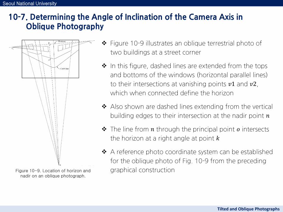
Figure 10-9 illustrates an oblique terrestrial photo of
two buildings at a street corner
In this figure, dashed lines are extended from the tops
and bottoms of the windows (horizontal parallel lines)
to their intersections at vanishing points 𝑣1 and 𝑣2,
which when connected define the horizon
Also shown are dashed lines extending from the vertical
building edges to their intersection at the nadir point 𝑛
The line from 𝑛 through the principal point 𝑜 intersects
the horizon at a right angle at point 𝑘
A reference photo coordinate system can be established
for the oblique photo of Fig. 10-9 from the preceding
graphical construction
10-7. Determining the Angle of Inclination of the Camera Axis in Oblique Photography
Seoul National University
Tilted and Oblique Photographs
Figure 10-9. Location of horizon and nadir on an oblique photograph.
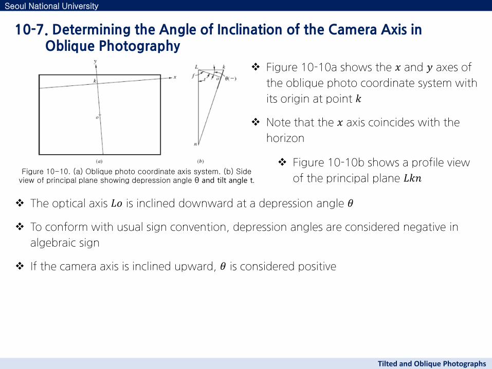
Figure 10-10a shows the 𝑥 and 𝑦 axes of
the oblique photo coordinate system with
its origin at point 𝑘
Note that the 𝑥 axis coincides with the
horizon
The optical axis 𝐿𝑜 is inclined downward at a depression angle 𝜃
To conform with usual sign convention, depression angles are considered negative in
algebraic sign
If the camera axis is inclined upward, 𝜃 is considered positive
10-7. Determining the Angle of Inclination of the Camera Axis in Oblique Photography
Seoul National University
Tilted and Oblique Photographs
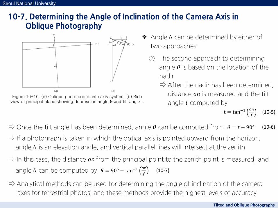
Figure 10-10. (a) Oblique photo coordinate axis system. (b) Side view of principal plane showing depression angle θ and tilt angle t.
Figure 10-10b shows a profile view
of the principal plane 𝐿𝑘𝑛
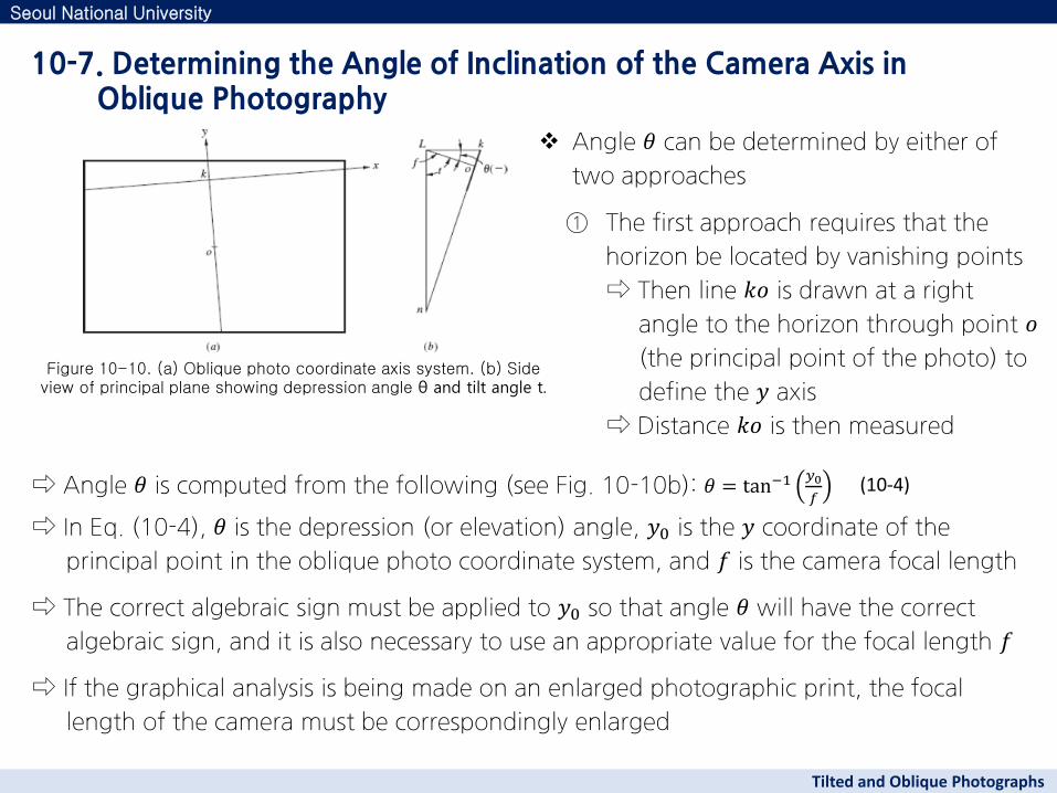
Angle 𝜃 can be determined by either of
two approaches
① The first approach requires that the
horizon be located by vanishing points
⇨ Then line 𝑘𝑜 is drawn at a right
angle to the horizon through point 𝑜
(the principal point of the photo) to
define the 𝑦 axis
⇨ Distance 𝑘𝑜 is then measured
10-7. Determining the Angle of Inclination of the Camera Axis in Oblique Photography
Seoul National University
Tilted and Oblique Photographs
Figure 10-10. (a) Oblique photo coordinate axis system. (b) Side view of principal plane showing depression angle θ and tilt angle t.
⇨ Angle 𝜃 is computed from the following (see Fig. 10-10b): 𝜃 = tan−1𝑦0
𝑓 (10-4)
⇨ In Eq. (10-4), 𝜃 is the depression (or elevation) angle, 𝑦0 is the 𝑦 coordinate of the
principal point in the oblique photo coordinate system, and 𝑓 is the camera focal length
⇨ The correct algebraic sign must be applied to 𝑦0 so that angle 𝜃 will have the correct
algebraic sign, and it is also necessary to use an appropriate value for the focal length 𝑓
⇨ If the graphical analysis is being made on an enlarged photographic print, the focal
length of the camera must be correspondingly enlarged
Angle 𝜃 can be determined by either of
two approaches
10-7. Determining the Angle of Inclination of the Camera Axis in Oblique Photography
Seoul National University
Tilted and Oblique Photographs
Figure 10-10. (a) Oblique photo coordinate axis system. (b) Side view of principal plane showing depression angle θ and tilt angle t.
② The second approach to determining
angle 𝜃 is based on the location of the
nadir
⇨ After the nadir has been determined,
distance 𝑜𝑛 is measured and the tilt
angle 𝑡 computed by
: t = tan−1𝑜𝑛
𝑓
(10-5)
⇨ Once the tilt angle has been determined, angle 𝜃 can be computed from 𝜃 = 𝑡 − 90° (10-6)
⇨ If a photograph is taken in which the optical axis is pointed upward from the horizon,
angle 𝜃 is an elevation angle, and vertical parallel lines will intersect at the zenith
⇨ In this case, the distance 𝑜𝑧 from the principal point to the zenith point is measured, and
angle 𝜃 can be computed by 𝜃 = 90° − tan−1𝑜𝑧
𝑓
⇨ Analytical methods can be used for determining the angle of inclination of the camera
axes for terrestrial photos, and these methods provide the highest levels of accuracy
(10-7)
Once angle 𝜃 has been determined,
horizontal and vertical angles can be
computed for points whose images appear
in the photograph
Refer to Fig. 10-8 which shows the
geometry of an oblique terrestrial
photograph
In this figure, 𝐿 is the exposure station, and 𝐿𝑜 is 𝑓 , the camera focal length; 𝐿𝑘 is a
horizontal line intersecting the photo at 𝑘
The 𝑥 axis coincides with the horizon line, and the 𝑦 axis passes through the principal
point 𝑜, perpendicular to the 𝑥 axis at point 𝑘
Point 𝑎 is an image point, and 𝑎𝑎′ is a vertical line, with 𝑎′ being located in the
horizontal plane of the exposure station and horizon line
10-8. Computing Horizontal and Vertical Angles from Oblique Photos
Seoul National University
Tilted and Oblique Photographs
Figure 10-8. Horizontal and vertical angles from measurements on an oblique terrestrial photo.
Horizontal angle 𝛼𝑎 between the vertical plane,
(𝐿𝑎′𝑎), containing image point 𝑎 and the
vertical plane, 𝐿𝑘𝑜, containing the camera axis is
Algebraic signs of 𝛼 angles are positive if they are clockwise from the optical axis and
negative if they are counterclockwise
After the horizontal angle 𝛼𝑎has been determined, vertical angle 𝛽𝑎 to image point 𝑎
can be calculated from the following equation:
The algebraic signs of 𝛽 angles are
automatically obtained from the signs
of the 𝑦 coordinates used in Eq. (10-9)
10-8. Computing Horizontal and Vertical Angles from Oblique Photos
Seoul National University
Tilted and Oblique Photographs
Figure 10-8. Horizontal and vertical angles from measurements on an oblique terrestrial photo.
(10-8)
In Eq. (10-8) note that correct algebraic signs
must be applied to 𝑥𝑎, 𝑦𝑎 and 𝜃
(10-9)
As previously stated, besides the tilt-swing-azimuth system, angular orientation of a
photograph can be expressed in terms of three rotation angles, 𝑜𝑚𝑒𝑔𝑎, 𝑝𝑖, and 𝑘𝑎𝑝𝑝𝑎
These three angles uniquely define the angular relationships between the three axes of
the photo (image) coordinate system and the three axes of the ground (object)
coordinate system
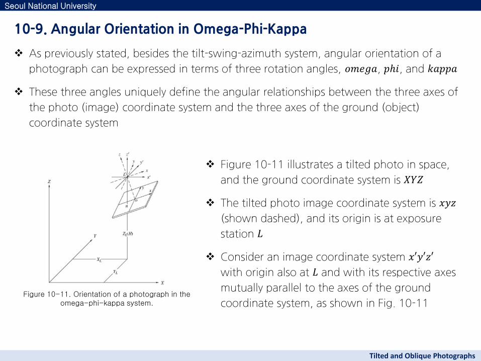
Figure 10-11 illustrates a tilted photo in space,
and the ground coordinate system is 𝑋𝑌𝑍
The tilted photo image coordinate system is 𝑥𝑦𝑧
(shown dashed), and its origin is at exposure
station 𝐿
Consider an image coordinate system 𝑥′𝑦′𝑧′
with origin also at 𝐿 and with its respective axes
mutually parallel to the axes of the ground
coordinate system, as shown in Fig. 10-11
10-9. Angular Orientation in Omega-Phi-Kappa
Seoul National University
Tilted and Oblique Photographs
Figure 10-11. Orientation of a photograph in the omega-phi-kappa system.
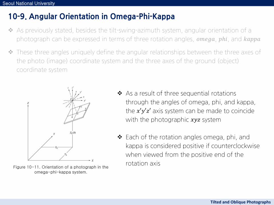
As a result of three sequential rotations
through the angles of omega, phi, and kappa,
the 𝑥′𝑦′𝑧′ axis system can be made to coincide
with the photographic 𝑥𝑦𝑧 system
Each of the rotation angles omega, phi, and
kappa is considered positive if counterclockwise
when viewed from the positive end of the
rotation axis
10-9. Angular Orientation in Omega-Phi-Kappa
Seoul National University
Tilted and Oblique Photographs
Figure 10-11. Orientation of a photograph in the omega-phi-kappa system.
As previously stated, besides the tilt-swing-azimuth system, angular orientation of a
photograph can be expressed in terms of three rotation angles, 𝑜𝑚𝑒𝑔𝑎, 𝑝𝑖, and 𝑘𝑎𝑝𝑝𝑎
These three angles uniquely define the angular relationships between the three axes of
the photo (image) coordinate system and the three axes of the ground (object)
coordinate system
The sequence of the three rotations is
illustrated in Fig. 10-12
The first rotation, as illustrated in Fig. 10-12a,
is about the 𝑥′ axis through an angle omega
This first rotation creates a new axis system
𝑥1𝑦1𝑧1
The second rotation phi is about the 𝑦1 axis, as
illustrated in Fig. 10-12b
As a result of the phi rotation a new axis system 𝑥1𝑦1𝑧1 is created
The third and final rotation is about the 𝑦1 axis through the angle kappa(Fig. 10-12c)
⇨ This third rotation creates the 𝑥𝑦𝑧 coordinate system which is the photographic
image system
10-9. Angular Orientation in Omega-Phi-Kappa
Seoul National University
Tilted and Oblique Photographs
Figure 10-12. (a) Rotation about the x’ axis through angle omega. (b) Rotation about the 𝑦1axis through angle phi. (c)
Rotation about the 𝑧2 axis through angle kappa.
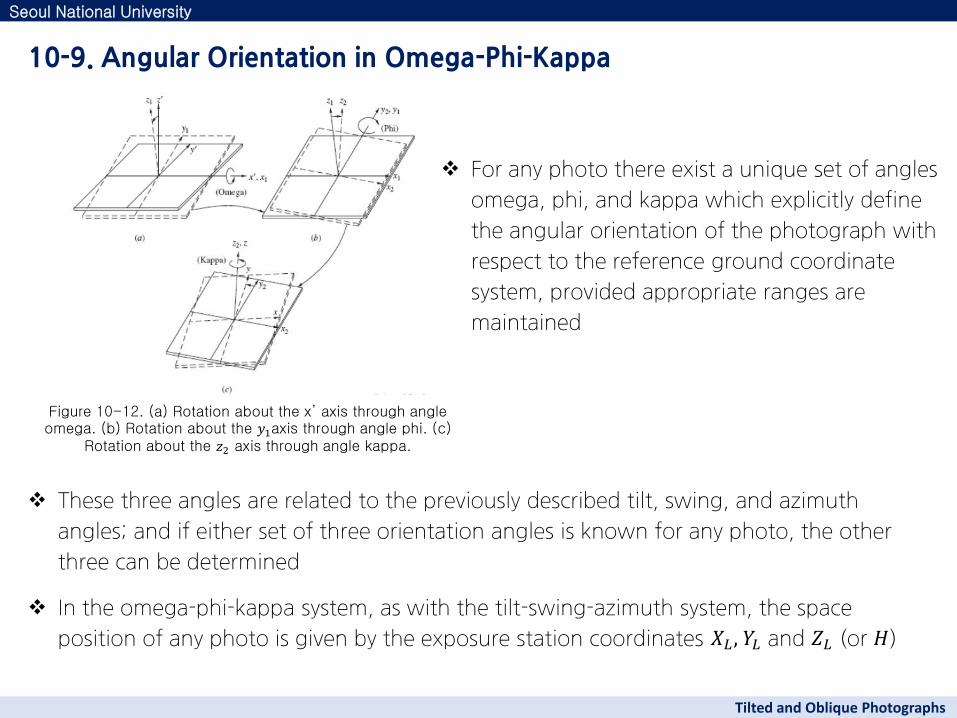
For any photo there exist a unique set of angles
omega, phi, and kappa which explicitly define
the angular orientation of the photograph with
respect to the reference ground coordinate
system, provided appropriate ranges are
maintained
10-9. Angular Orientation in Omega-Phi-Kappa
Seoul National University
Tilted and Oblique Photographs
Figure 10-12. (a) Rotation about the x’ axis through angle omega. (b) Rotation about the 𝑦1axis through angle phi. (c)
Rotation about the 𝑧2 axis through angle kappa.
These three angles are related to the previously described tilt, swing, and azimuth
angles; and if either set of three orientation angles is known for any photo, the other
three can be determined
In the omega-phi-kappa system, as with the tilt-swing-azimuth system, the space
position of any photo is given by the exposure station coordinates 𝑋𝐿 , 𝑌𝐿 and 𝑍𝐿 (or 𝐻)
Many different methods, both graphical and numerical, have been devised to
determine the six elements of exterior orientation of a single photograph
In general all methods require photographic images of at least three control points
whose 𝑋, 𝑌, and 𝑍 ground coordinates are known, and the calibrated focal length of
the camera must be known
Although the most commonly used method to find these elements is space resection
by collinearity
The method of space resection by collinearity is a purely numerical method which
simultaneously yields all six elements of exterior orientation
Normally the angular values of omega, phi, and kappa are obtained in the solution,
although the method is versatile and tilt, swing, and azimuth could also be obtained
10-10. Determining the Elements of Exterior Orientation
Seoul National University
Tilted and Oblique Photographs
Space resection by collinearity permits the use of redundant amounts of ground
control; hence least squares computational techniques can be used to determine most
probable values for the six elements
This method is a rather lengthy procedure requiring an iterative solution of nonlinear
equations, but when programmed for a computer, a solution is easily obtained
Space resection by collinearity involves formulating the so-called collinearity equations
for a number of control points whose 𝑋, 𝑌, and 𝑍 ground coordinates are known and
whose images appear in the photo
The equations are then solved for the six unknown elements of exterior orientation
which appear in them
The collinearity equations express the condition that for any given photograph the
exposure station, any object point and its corresponding image all lie on a straight line
10-10. Determining the Elements of Exterior Orientation
Seoul National University
Tilted and Oblique Photographs
Rectification is the process of making equivalent vertical photographs from tilted photo
negatives
The resulting equivalent vertical photos are called rectified photographs
Rectified photos theoretically are truly vertical photos, and as such they are free from
displacements of images due to tilt
⇨ They do, however, still contain image displacements and scale variations due to
topographic relief
⇨ These relief displacements and scale variations can also be removed in a process called
differential rectification or orthorectification, and the resulting products are then
called orthophotos
Orthophotos are often preferred over rectified photos because of their superior
geometric quality
⇨ Nevertheless, rectified photos are still quite popular because they do make very good
map substitutes where terrain variations are moderate
10-11. Rectification of Tilted Photographs
Seoul National University
Tilted and Oblique Photographs
Rectification is generally performed by any of three methods:
analytically, optically-mechanically, and digital
1) Analytical rectification has the disadvantage that it can be applied only to individual
discrete points
The resulting rectified photos produced by analytical methods are not really photos
at all since they are not composed of photo images
Rather, they are plots of individual points in their rectified locations
2) The optical-mechanical and digital methods produce an actual picture in which the
images of the tilted photo have been transformed to their rectified locations
The products of these two methods can be used in the production of photomaps
and mosaics. In any of these rectification procedures, the rectified photos can be
simultaneously ratioed
This is particularly advantageous if rectified photos are being made for the purpose
of constructing a controlled mosaic, since all photos in the strip of block can be
brought to a common scale
Thus, the resulting mosaic will have a more uniform scale throughout
10-11. Rectification of Tilted Photographs
Seoul National University
Tilted and Oblique Photographs
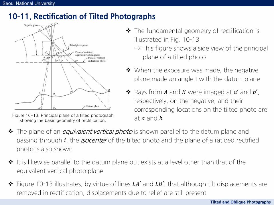
The fundamental geometry of rectification is
illustrated in Fig. 10-13
⇨ This figure shows a side view of the principal
plane of a tilted photo
When the exposure was made, the negative
plane made an angle t with the datum plane
Rays from 𝐴 and 𝐵 were imaged at 𝑎′ and 𝑏′,
respectively, on the negative, and their
corresponding locations on the tilted photo are
at 𝑎 and 𝑏
The plane of an equivalent vertical photo is shown parallel to the datum plane and
passing through 𝑖, the isocenter of the tilted photo and the plane of a ratioed rectified
photo is also shown
It is likewise parallel to the datum plane but exists at a level other than that of the
equivalent vertical photo plane
Figure 10-13 illustrates, by virtue of lines 𝐿𝐴′ and 𝐿𝐵′, that although tilt displacements are
removed in rectification, displacements due to relief are still present
10-11. Rectification of Tilted Photographs
Seoul National University
Tilted and Oblique Photographs
Figure 10-13. Principal plane of a tilted photograph showing the basic geometry of rectification.
Since rectified and ratioed aerial photos retain the effects of relief, ground control points
used in rectification must be adjusted slightly to accommodate their relief displacements
Conceptually, the process involves plotting ground control points at the locations that
they will occupy in the rectified and ratioed photo
To this end, the positional displacements due to relief of the control points must be
computed and applied to their horizontal positions in a radial direction from the exposure
station so that they will line up with points in the rectified photo
This procedure requires that the coordinates 𝑋𝐿 , 𝑌𝐿, and 𝑍𝐿 (or 𝐻) of the exposure station
(which can be computed by space resection) and the 𝑋, 𝑌,and 𝑍 (or ) coordinates for
each ground control point be known
In addition, when the rectified photos are to be ratioed as well, it is convenient to select a
plane in object space, at a specified elevation, to which the scale of the ratioed photo will
be related
Generally, the elevation of this plane will be chosen as the elevation of average terrain,
𝑎𝑣𝑔
10-12. Correction for Relief of Ground Control Points Used in Rectification
Seoul National University
Tilted and Oblique Photographs
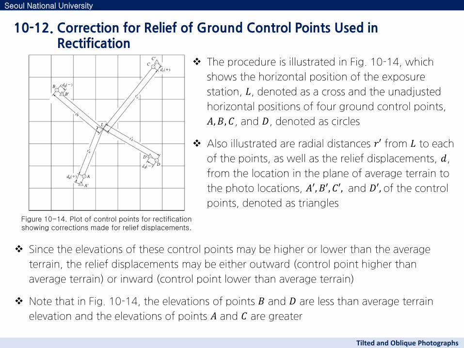
The procedure is illustrated in Fig. 10-14, which
shows the horizontal position of the exposure
station, 𝐿, denoted as a cross and the unadjusted
horizontal positions of four ground control points,
𝐴, 𝐵, 𝐶, and 𝐷, denoted as circles
Also illustrated are radial distances 𝑟′ from 𝐿 to each
of the points, as well as the relief displacements, 𝑑,
from the location in the plane of average terrain to
the photo locations, 𝐴′, 𝐵′, 𝐶′, and 𝐷′,of the control
points, denoted as triangles
Since the elevations of these control points may be higher or lower than the average
terrain, the relief displacements may be either outward (control point higher than
average terrain) or inward (control point lower than average terrain)
Note that in Fig. 10-14, the elevations of points 𝐵 and 𝐷 are less than average terrain
elevation and the elevations of points 𝐴 and 𝐶 are greater
Seoul National University
Tilted and Oblique Photographs
Figure 10-14. Plot of control points for rectification showing corrections made for relief displacements.
10-12. Correction for Relief of Ground Control Points Used in Rectification
Determination of the coordinates of a displaced point (triangle) involves several steps
Initially, the value of 𝑟′ is computed by Eq. (10-10) using the point's horizontal
coordinates 𝑋 and 𝑌, and the horizontal coordinates of the exposure station, 𝑋𝐿 and 𝑌𝐿
The relief displacement, 𝑑 , is calculated by Eq. (10-11), which is a variation of Eq. (6-11):
Seoul National University
Tilted and Oblique Photographs
(10-10)
(10-11)
𝑑 =𝑟
𝐻 (6-11)
where 𝑑=relief displacement = height above datum of object point whose image is displaced 𝑟 = radial distance on photograph from principal point to displaced image (The units of 𝑑 and 𝑟 must be the same.) 𝐻 = flying height above same datum selected for measurement of
10-12. Correction for Relief of Ground Control Points Used in Rectification
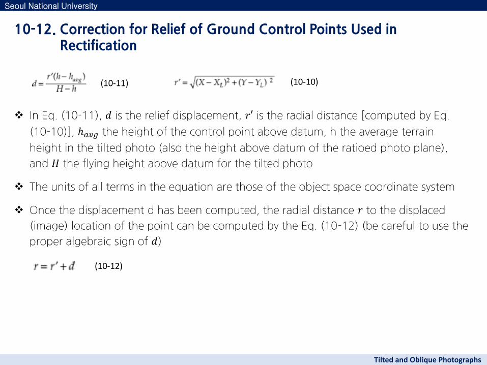
In Eq. (10-11), 𝑑 is the relief displacement, 𝑟′ is the radial distance [computed by Eq.
(10-10)], 𝑎𝑣𝑔 the height of the control point above datum, h the average terrain
height in the tilted photo (also the height above datum of the ratioed photo plane),
and 𝐻 the flying height above datum for the tilted photo
The units of all terms in the equation are those of the object space coordinate system
Once the displacement d has been computed, the radial distance 𝑟 to the displaced
(image) location of the point can be computed by the Eq. (10-12) (be careful to use the
proper algebraic sign of 𝑑)
Seoul National University
Tilted and Oblique Photographs
(10-12)
(10-10) (10-11)
10-12. Correction for Relief of Ground Control Points Used in Rectification
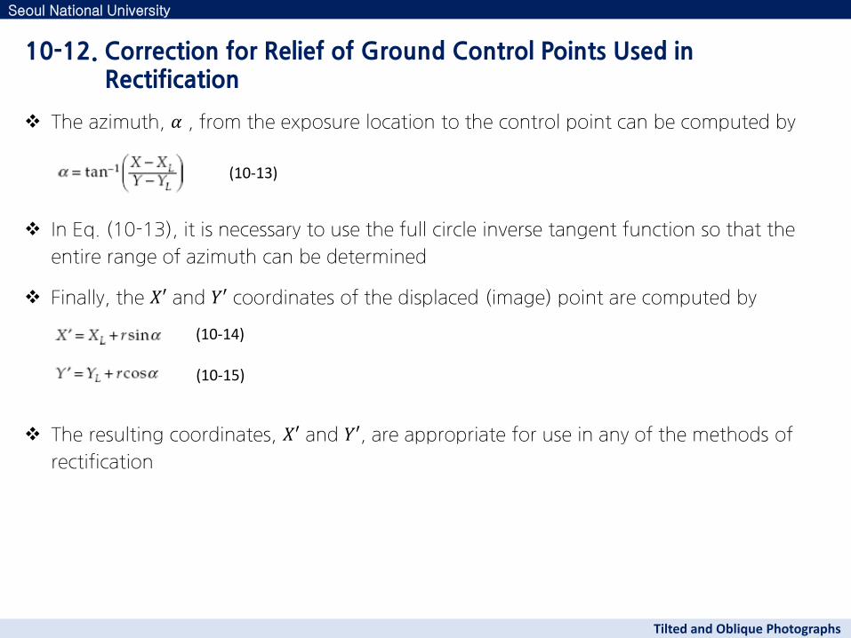
The azimuth, 𝛼 , from the exposure location to the control point can be computed by
The resulting coordinates, 𝑋′ and 𝑌′, are appropriate for use in any of the methods of
rectification
Seoul National University
Tilted and Oblique Photographs
10-12. Correction for Relief of Ground Control Points Used in Rectification
(10-13)
In Eq. (10-13), it is necessary to use the full circle inverse tangent function so that the
entire range of azimuth can be determined
Finally, the 𝑋′ and 𝑌′ coordinates of the displaced (image) point are computed by
(10-14)
(10-15)
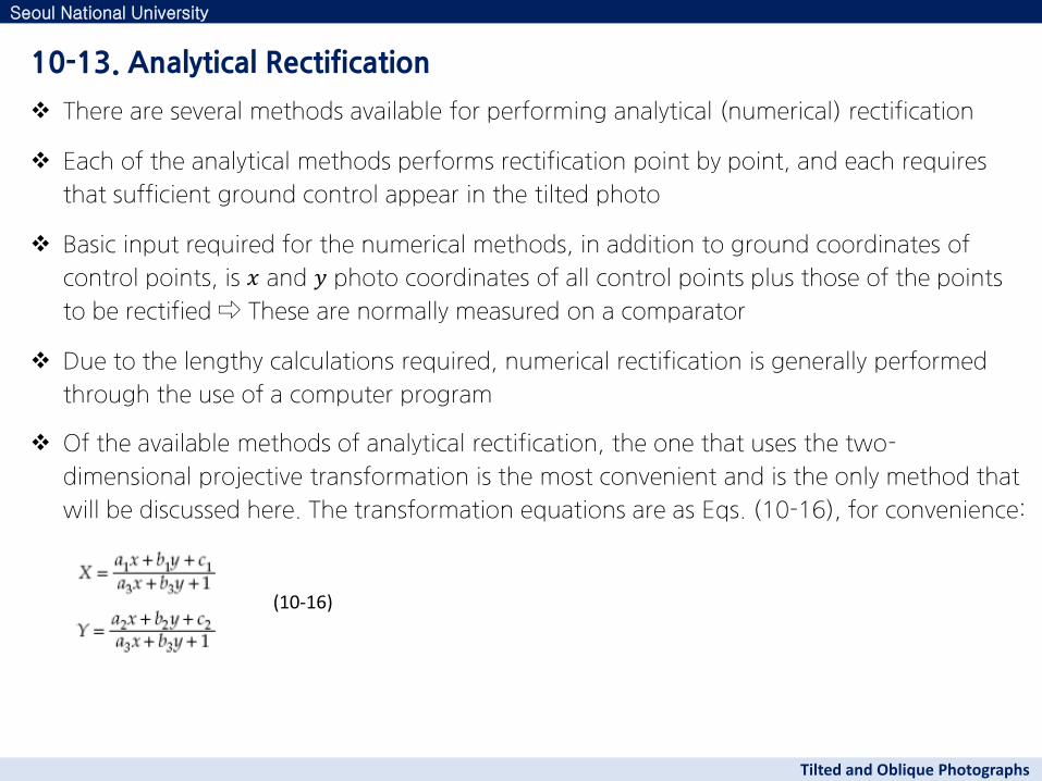
There are several methods available for performing analytical (numerical) rectification
Each of the analytical methods performs rectification point by point, and each requires
that sufficient ground control appear in the tilted photo
Basic input required for the numerical methods, in addition to ground coordinates of
control points, is 𝑥 and 𝑦 photo coordinates of all control points plus those of the points
to be rectified ⇨ These are normally measured on a comparator
Due to the lengthy calculations required, numerical rectification is generally performed
through the use of a computer program
Of the available methods of analytical rectification, the one that uses the two-
dimensional projective transformation is the most convenient and is the only method that
will be discussed here. The transformation equations are as Eqs. (10-16), for convenience:
10-13. Analytical Rectification
Seoul National University
Tilted and Oblique Photographs
(10-16)
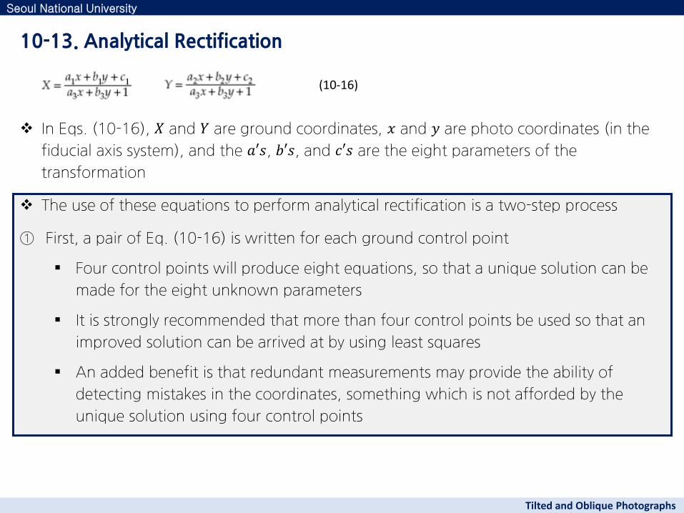
In Eqs. (10-16), 𝑋 and 𝑌 are ground coordinates, 𝑥 and 𝑦 are photo coordinates (in the
fiducial axis system), and the 𝑎′𝑠, 𝑏′𝑠, and 𝑐′𝑠 are the eight parameters of the
transformation
The use of these equations to perform analytical rectification is a two-step process
① First, a pair of Eq. (10-16) is written for each ground control point
Four control points will produce eight equations, so that a unique solution can be
made for the eight unknown parameters
It is strongly recommended that more than four control points be used so that an
improved solution can be arrived at by using least squares
An added benefit is that redundant measurements may provide the ability of
detecting mistakes in the coordinates, something which is not afforded by the
unique solution using four control points
10-13. Analytical Rectification
Seoul National University
Tilted and Oblique Photographs
(10-16)
In Eqs. (10-16), 𝑋 and 𝑌 are ground coordinates, 𝑥 and 𝑦 are photo coordinates (in the
fiducial axis system), and the 𝑎′𝑠, 𝑏′𝑠, and 𝑐′𝑠 are the eight parameters of the
transformation
The use of these equations to perform analytical rectification is a two-step process
② Once the eight parameters have been determined, the second step of the solution can
be performed
Solving Eqs. (10-16) for each point whose 𝑋 and 𝑌 rectified coordinates are desired
After rectified coordinates have been computed in the ground coordinate system,
they can be plotted at the scale desired for the rectified and ratioed photo
This analytical method is only rigorous if the ground coordinates, 𝑋 and 𝑌, of Eqs.
(10-16) have been modified for relief displacements
If this is not done, a quasi-rectification results; although if the terrain is relatively flat
and level, the errors will be minimal
10-13. Analytical Rectification
Seoul National University
Tilted and Oblique Photographs
(10-16)
In practice, the optical-mechanical method is still being used, although digital methods
have rapidly surpassed this approach
The optical-mechanical method relies on instruments called rectifiers
They produce rectified and ratioed photos through the photographic process of
projection printing ⇨ thus they must be operated in a darkroom
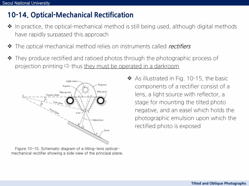
As illustrated in Fig. 10-15, the basic
components of a rectifier consist of a
lens, a light source with reflector, a
stage for mounting the tilted photo
negative, and an easel which holds the
photographic emulsion upon which the
rectified photo is exposed
10-14. Optical-Mechanical Rectification
Seoul National University
Tilted and Oblique Photographs
Figure 10-15. Schematic diagram of a tilting-lens optical-mechanical rectifier showing a side view of the principal plane.
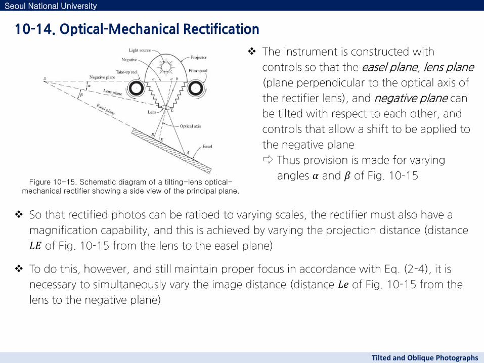
The instrument is constructed with
controls so that the easel plane, lens plane
(plane perpendicular to the optical axis of
the rectifier lens), and negative plane can
be tilted with respect to each other, and
controls that allow a shift to be applied to
the negative plane
⇨ Thus provision is made for varying
angles 𝛼 and 𝛽 of Fig. 10-15
10-14. Optical-Mechanical Rectification
Seoul National University
Tilted and Oblique Photographs
Figure 10-15. Schematic diagram of a tilting-lens optical-mechanical rectifier showing a side view of the principal plane.
So that rectified photos can be ratioed to varying scales, the rectifier must also have a
magnification capability, and this is achieved by varying the projection distance (distance
𝐿𝐸 of Fig. 10-15 from the lens to the easel plane)
To do this, however, and still maintain proper focus in accordance with Eq. (2-4), it is
necessary to simultaneously vary the image distance (distance 𝐿𝑒 of Fig. 10-15 from the
lens to the negative plane)
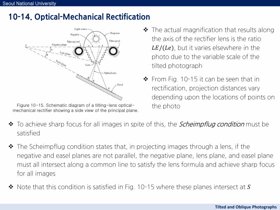
The actual magnification that results along
the axis of the rectifier lens is the ratio
𝐿𝐸/(𝐿𝑒), but it varies elsewhere in the
photo due to the variable scale of the
tilted photograph
From Fig. 10-15 it can be seen that in
rectification, projection distances vary
depending upon the locations of points on
the photo
10-14. Optical-Mechanical Rectification
Seoul National University
Tilted and Oblique Photographs
Figure 10-15. Schematic diagram of a tilting-lens optical-mechanical rectifier showing a side view of the principal plane.
To achieve sharp focus for all images in spite of this, the Scheimpflug condition must be
satisfied
The Scheimpflug condition states that, in projecting images through a lens, if the
negative and easel planes are not parallel, the negative plane, lens plane, and easel plane
must all intersect along a common line to satisfy the lens formula and achieve sharp focus
for all images
Note that this condition is satisfied in Fig. 10-15 where these planes intersect at 𝑆

Rectified photos can be produced by digital techniques that incorporate a
photogrammetric scanner and computer processing
⇨ This procedure is a special case of the more general concept of georeferencing
Rectification requires that a projective transformation be used to relate the image to the
ground coordinate system whereas georeferencing often uses simpler transformations
such as the two-dimensional conformal or the two-dimensional affine transformation
10-15. Digital Rectification
Seoul National University
Tilted and Oblique Photographs
Figure 10-16. (a) Digital image of an oblique, nonrectified photograph. (b) Image after digital rectification.
Figure 10-16a shows a portion of a
scanned aerial oblique
Note that images in the foreground
(near the bottom) are at a larger scale
than those near the top
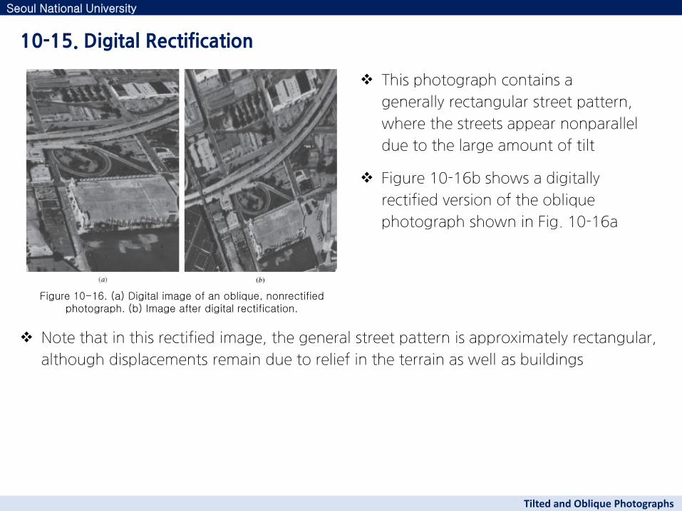
This photograph contains a
generally rectangular street pattern,
where the streets appear nonparallel
due to the large amount of tilt
Figure 10-16b shows a digitally
rectified version of the oblique
photograph shown in Fig. 10-16a
Note that in this rectified image, the general street pattern is approximately rectangular,
although displacements remain due to relief in the terrain as well as buildings
10-15. Digital Rectification
Seoul National University
Tilted and Oblique Photographs
Figure 10-16. (a) Digital image of an oblique, nonrectified photograph. (b) Image after digital rectification.
Three primary pieces of equipment needed for digital rectification are a digital image
(either taken from a digital camera or a scanned photo), computer, and plotting device
capable of producing digital image output
While a high-quality photogrammetric scanner is an expensive device, it is also highly
versatile and can be used for many other digital-photogrammetric operations
Low-accuracy desktop scanners can also be used for digital rectification
⇨ However, the geometric accuracy of the product will be substantially lower
Current plotting devices, generally large-format ink jet printers, produce image output
of good quality, although the geometric accuracy and image resolution may be slightly
less than that of photographic rectifiers
10-15. Digital Rectification
Seoul National University
Tilted and Oblique Photographs

Atmospheric refraction in aerial photographs occurs radially from the nadir point
Now that parameters of tilted photographs have been described, a technique that
corrects image coordinates in a tilted photo for the effects of atmospheric refraction is
presented
In most practical situations, the assumption of vertical photography is sufficient when
calculating atmospheric refraction
However for highest accuracy, when dealing with high altitude photography (e.g.,
flying height greater than 5000 m) and photographs with excessive tilts (e.g., tilts
greater than 5°) should be considered when atmospheric refraction corrections are
made
10-16. Atmospheric Rectification in Tilted Aerial Photographs
Seoul National University
Tilted and Oblique Photographs
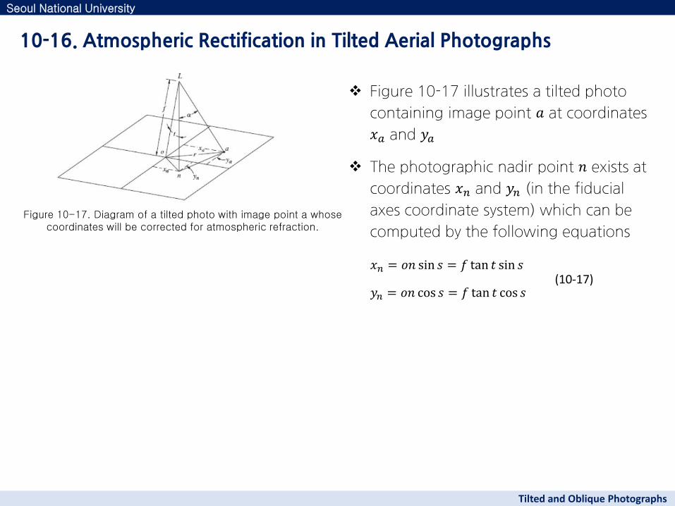
Figure 10-17 illustrates a tilted photo
containing image point 𝑎 at coordinates
𝑥𝑎 and 𝑦𝑎
The photographic nadir point 𝑛 exists at
coordinates 𝑥𝑛 and 𝑦𝑛 (in the fiducial
axes coordinate system) which can be
computed by the following equations
10-16. Atmospheric Rectification in Tilted Aerial Photographs
Seoul National University
Tilted and Oblique Photographs
Figure 10-17. Diagram of a tilted photo with image point a whose coordinates will be corrected for atmospheric refraction.
𝑥𝑛 = 𝑜𝑛 sin 𝑠 = 𝑓 tan 𝑡 sin 𝑠
𝑦𝑛 = 𝑜𝑛 cos 𝑠 = 𝑓 tan 𝑡 cos 𝑠 (10-17)
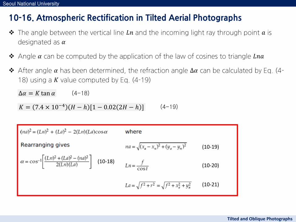
The angle between the vertical line 𝐿𝑛 and the incoming light ray through point 𝑎 is
designated as 𝛼
Angle 𝛼 can be computed by the application of the law of cosines to triangle 𝐿𝑛𝑎
After angle 𝛼 has been determined, the refraction angle Δ𝛼 can be calculated by Eq. (4-
18) using a 𝐾 value computed by Eq. (4-19)
10-16. Atmospheric Rectification in Tilted Aerial Photographs
Seoul National University
Tilted and Oblique Photographs
(10-18)
(10-19)
(10-20)
(10-21)
∆𝛼 = 𝐾 tan 𝛼 (4-18)
𝐾 = 7.4 × 10⁻⁴ 𝐻 − [1 − 0.02 2𝐻 − ] (4-19)
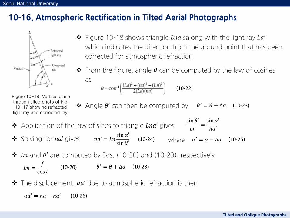
Figure 10-18 shows triangle 𝐿𝑛𝑎 salong with the light ray 𝐿𝑎′
which indicates the direction from the ground point that has been
corrected for atmospheric refraction
From the figure, angle 𝜃 can be computed by the law of cosines
as
Angle 𝜃′ can then be computed by
Application of the law of sines to triangle 𝐿𝑛𝑎′ gives
10-16. Atmospheric Rectification in Tilted Aerial Photographs
Seoul National University
Tilted and Oblique Photographs
Figure 10-18. Vertical plane through tilted photo of Fig. 10-17 showing refracted
light ray and corrected ray.
𝜃′ = 𝜃 + ∆𝛼 (10-23)
(10-22)
sin 𝜃′
𝐿𝑛=sin 𝛼′
𝑛𝑎′
Solving for 𝑛𝑎’ gives 𝑛𝑎′ = 𝐿𝑛sin 𝛼′
sin 𝜃′ (10-24) where 𝛼′ = 𝛼 − ∆𝛼 (10-25)
𝑎𝑎′ = 𝑛𝑎 − 𝑛𝑎′ (10-26)
𝐿𝑛 and 𝜃′ are computed by Eqs. (10-20) and (10-23), respectively
The displacement, 𝑎𝑎′ due to atmospheric refraction is then
(10-20) 𝐿𝑛 =𝑓
cos 𝑡 𝜃′ = 𝜃 + ∆𝛼 (10-23)
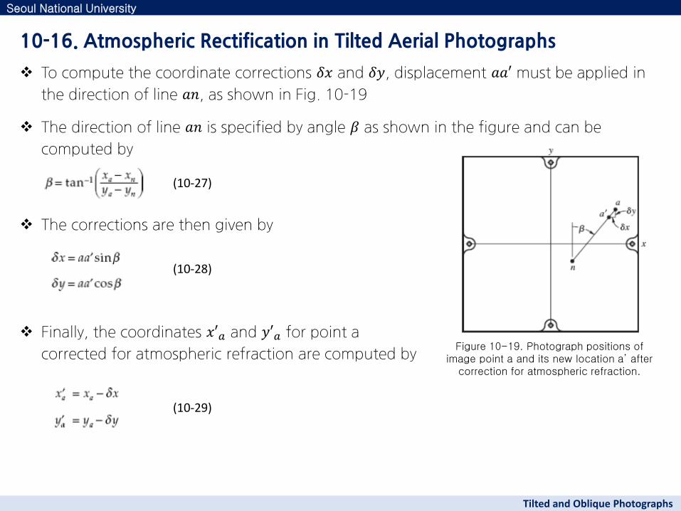
To compute the coordinate corrections 𝛿𝑥 and 𝛿𝑦, displacement 𝑎𝑎′ must be applied in
the direction of line 𝑎𝑛, as shown in Fig. 10-19
The direction of line 𝑎𝑛 is specified by angle 𝛽 as shown in the figure and can be
computed by
The corrections are then given by
Finally, the coordinates 𝑥′𝑎 and 𝑦′𝑎 for point a
corrected for atmospheric refraction are computed by
10-16. Atmospheric Rectification in Tilted Aerial Photographs
Seoul National University
Tilted and Oblique Photographs
Figure 10-19. Photograph positions of image point a and its new location a’ after
correction for atmospheric refraction.
(10-27)
(10-29)
(10-28)
Two final comments regarding refraction in a tilted photo are in order
1) The values of tilt and swing are not known until after an analytical solution is performed
⇨ However, photo coordinates are necessary in order to compute the analytical solution
⇨ Therefore refinement for atmospheric refraction in a tilted photograph must be
performed in an iterative fashion
⇨ Since analytical photogrammetric solutions are generally iterative due to the nonlinear
equations involved, tilted photo refraction corrections can be conveniently inserted into
the iterative loop
2) The foregoing discussion of atmospheric refraction in a tilted photograph assumes that
the tilt angle is the angle between the optical axis and a vertical line
⇨ In analytical photogrammetry, a local vertical coordinate system is generally used for
object space
⇨ As a result, tilt angles will be related to the direction of the local vertical Z axis which is
generally different from the true vertical direction
⇨ This effect is negligible for practical situations
⇨ Unless a photograph is more than about 300 km from the local vertical origin, the
effect from ignoring this difference in vertical direction will generally be less than
0.001 mm
10-16. Atmospheric Rectification in Tilted Aerial Photographs
Seoul National University
Tilted and Oblique Photographs


