This chapter focuses on Received Signal Strength (RSS) based indoor positioning.It first provides an overview of various indoor localization techniques employing RSSincluding lateration methods, machine learning classification, probabilistic approaches,and statistical supervised learning techniques. It then compares their performance interms of localization accuracy through measurement studies in real office building en-vironments under representative WiFi and ZigBee wireless networks. It further surveystechniques and methods that are developed to support robust wireless localization andimprove localization accuracy, including real-time RSS calibration via anchor verifica-tion, closely spaced multiple antennas, taking advantage of robust statistical methodsto provide stability to contaminated measurements, utilizing linear regression to char-acterize the relationship between RSS and the distance to anchors, and exploiting RSSspatial correlation. Finally, it concludes with a discussion of popular location-basedapplications.
12.1 Introduction
The widespread deployment of indoor wireless technologies is resulting in a variety oflocation-based services. For instance, in the public arena doctors want to use locationinformation to track and monitor patients in medical facilities and first responders needto track each other and locate victims during emergency rescues. On the other hand, in
1
the enterprise domain, location-based access control is desirable for accessing proprietarycorporate materials in restricted areas or rooms. For example, during corporate meetings,certain documents can only be received by laptops reside within the involved conferencerooms, which requires location-aware content delivery. In addition, asset tracking alsorelies on location information. To ensure the wide deployment of these pervasive ap-plications, accurate positioning is important as the location is a critical input to manyhigh-level tasks supporting these applications. In addition, in indoor environments, suchas shopping malls, hospitals, warehouses, and factories, where Global Positioning System(GPS) devices generally do not work, indoor localization systems promise the benefitsof accurate location estimates for wireless devices such as handheld devices, electronicbadges and laptop computers.
Compared to various physical modalities for localization, such as Time of Arrival(ToA) [1], Time Difference of Arrival (TDoA) [2], and Angle of Arrival (AoA), using theReceived Signal Strength (RSS) [3–5] is an attractive approach to perform localizationsince it can reuse the existing wireless infrastructures, and thus presents tremendouscost savings over deploying localization-specific hardware. Also, all current standardcommodity radio technologies, such as WiFi, ZigBee, active RFID, and Bluetooth provideRSS measurements, and consequently the same algorithms can be applied across differentplatforms.
Performing RSS-based localization is a challenging task due to multipath effects inunpredictable indoor settings. These effects include shadowing, i.e., blocking a signal,reflection, i.e., waves bouncing off an object, diffraction, i.e., waves spreading in re-sponse to obstacles, and refraction, i.e., waves bending as they pass through differentmediums. Thus, the RSS measurements will be attenuated in unpredictable ways dueto these effects. To tackle these challenges, recent studies have resulted in a plethora ofmethods for localizing wireless devices using RSS. This chapter provides an overview ofvarious indoor localization techniques employing RSS including lateration methods, ma-chine learning classification, probabilistic approaches, and statistical supervised learningtechniques. We then study the localization performance by presenting representativeevaluation metrics. We further compare the performance of various localization algo-rithms in terms of localization accuracy through real office building environments usingprevailing WiFi and ZigBee wireless networks.
Furthermore, we survey techniques and methods that are developed to support ro-bust wireless localization and improve localization accuracy, including real-time RSScalibration via anchor verification, multiple closely spaced antennas, taking advantageof the robust statistical methods to provide stability to contaminated measurements,utilizing linear regression to characterize the relationship between RSS and the distanceto anchors more accurately, and exploiting RSS spatial correlation. Finally, we concludethe chapter by presenting current and emerging applications that leverage the locationinformation.
2
12.2 RSS-based Localization Algorithms
An indoor positioning system consists of a set of anchor nodes (e.g. WiFi access pointsor traffic sniffers) placed at known locations in the area of interest, and a wireless devicecarried by the person or attached to the object that needs to be localized. During theoperation of localization, radio signals are transmitted between the wireless device andmultiple anchors. Based on the received wireless signal at either the anchors or thewireless device, a localization algorithm estimates the position of the wireless device.We next describe a generalized localization model that the localization algorithms arebased upon to map the observed RSS in signal space to the physical location in thephysical space [5].
In a generalized localization model, let us suppose that we have a domain D in two-dimensions, such as an office building, over which we wish to localize wireless devices.Within D, a set of n anchor points are available to assist in localization. A wireless devicethat transmits with a fixed power in an isotropic manner will cause a vector of n signalstrength readings to be measured by the n anchor points. In practice, these n signalstrength readings are averaged over a sufficiently large time window to remove statisticalvariability. Therefore, corresponding to each location in D, there is an n-dimensionalvector of signal readings s = (s1, s2, · · · , sn) that resides in a range R.
This relationship between positions in D and signal strength vectors defines a fin-gerprint function F : D → R that takes our real world position (x, y) and maps it to asignal strength reading s. F has some important properties. First, in practice, F is notcompletely specified, but rather a finite set of positions (xj , yj) is used for measuring acorresponding set of signal strength vectors sj . Additionally, the function F is generallyone-to-one, but is not onto. This means that the inverse of F is a function G that is notwell-defined: There are holes in the n-dimensional space in which R resides for whichthere is no well-defined inverse.
It is precisely the inverse function G, though, that allows us to perform localization.In general, we will have a signal strength reading s for which there is no explicit inverse(e.g. perhaps due to noise variability). Instead of using G, which has a domain restrictedto R, we consider various pseudo-inverses Galg of F for which the domain of Galg is thecomplete n-dimensional space. Here, the notation Galg indicates that there are differentalgorithmic choices, i.e., various localization algorithms, for the pseudo-inverse.
We use signal strength to illustrate the generalized localization model is becausesignal strength is a common wireless signal modality used by a widely diverse set oflocalization algorithms. For instance, radio-frequency (RF) fingerprinting approachesutilize RSS [3, 6], and many lateration approaches [7] use it as well1. In spite of itsseveral meter-level accuracy, using RSS is a natural choice because it can re-use theexisting wireless infrastructure and this feature presents a tremendous cost savings overdeploying localization-specific hardware. We next provide an overview of a representativeset of algorithms using RSS to perform position estimation.
1Chapter 15 describes fingerprinting approaches in more detail and Chapter 6 describes lateration
approaches in more detail.
3
12.2.1 Approach Overview
There are several ways to classify localization algorithms that use signal strength: range-based schemes, which explicitly involve the calculation of distances to landmarks; and RFfingerprinting schemes which originated from machine learning classification, whereby aradio map is constructed using prior measurements, and a device is localized by refer-encing this radio map through classification. We provide an overview of various indoorlocalization techniques employing RSS including lateration methods, machine learningclassification, probabilistic approaches, and statistical supervised learning techniques.They can be further categorized as range-based methods, such as lateration methods andBayesian Networks, and RF fingerprinting strategies, including fingerprinting matchingusing machine learning classification and maximum likelihood estimation using proba-bilistic approaches.
In lateration methods, the RSS measurements are used to perform ranging betweenthe wireless device and anchor points based on fitting a signal propagation model, andthen the location of the wireless device can be computed via trilateration.
For the machine learning classification via fingerprinting matching, it first builds apriori radio signal strength map of the localization region during the training phasebased on the measured signal strengths (i.e. RF fingerprints) at different locations. Bycomparing the online measured RSS to the pre-constructed signal map using some opti-mization criterion, the location can be deduced. For example, the minimum Euclideandistance in the signal-strength vector space can be used as an optimization criterion asdescribed in RADAR [3]. In these approaches location estimation is only consideredthrough the value of the RSS measurements.
On the other hand, probabilistic approaches have been proposed, where the RSS istreated as a random variable that may be modeled by a log-normal distribution [8] ata specific location. In these approaches, a signal strength probability distribution basedon the RSS measurements is modeled. During the localization phase, the position ofthe targeted wireless device is estimated using probabilistic methods, such as maximumlikelihood estimation.
In addition, Bayesian Networks and Kernel methods (which is discussed in ChapterXX) are methods that utilize the statistical supervised learning approach [9]. In statisti-cal supervised learning, it infers a function from supervised training data. The trainingdata consist of a set of training examples including input vectors, such as the RSS froma set of anchors and a desired output value (i.e. the location of the wireless device).The localization algorithms that perform supervised learning analyze the training dataand produce an inferred function, which is called a classifier that predicts the locationof wireless device for any valid input RSS vectors. We will now examine each class ofalgorithms in more detail.
12.2.2 Lateration Methods
Lateration is the most common method for deriving the location of a wireless device [10–12]. By estimating the distance from a wireless device to multiple anchors, laterationapproaches derive the wireless device’s location based on least squares methods.
4
In particular, RSS is employed to estimate the distance between a wireless device andan anchor. We next show an example on how to use off-line training phase to estimatethe propagation model parameters so as to derive ranging information from the measuredRSS during runtime localization phase. We note that there are some approaches treatthe propagation model parameters as nuisance parameters that are examined along withthe position2.
Example 12.1 Parameter estimation in the signal propagation model
In this example, we show that the radio propagation parameters can be estimatedfrom the training data collected during the off-line training phase.
Solution: During the off-line training phase, RSS samples are collected at variousknown locations from multiple anchors and distances are calculated from the knownlocations to anchors. The measured RSS readings and the corresponding distancesare then used to fit the signal propagation model based on the signal-to-distancerelationship [8, 13]:
P (d)[dBm] = P (d0)[dBm] − 10γ log10
(
d
d0
)
+ Xσ, (12.1)
where P (d0) represents the received power of a wireless device at the reference dis-tance d0, d is the distance between the wireless device and the anchor, γ is the pathloss exponent and Xσ is the shadow fading, which follows zero mean Gaussian dis-tribution with σ standard deviation. Given the RSS and distances, linear regressionis usually used to fit the propagation model [14].
During the runtime localization phase, there are two steps: ranging and lateration.In the ranging step, according to the measured RSS from the targeting wireless deviceand the fitted signal-to-distance relationship (i.e. the propagation model parameters),the distances between the wireless device and multiple anchors can be calculated. Inthe lateration step, the location of the wireless device can be estimated according todistances between the wireless device and the anchors based on least squares methods.In the literature, there are two popular methods: Non-Linear Least Square (NLS) andLinear Least Square (LLS), in the lateration step.
Non-Linear Least Square (NLS): Given the estimated distances di from thetargeting device to anchors and known positions (xi, yi) of the anchors, the position(x, y) of the wireless device can be estimated by finding (x, y) satisfying:
(x, y) = arg minx,y
N∑
i=1
[√
(xi − x)2 + (yi − y)2 − di2)] (12.2)
where N is the number of anchors that are chosen to estimate the position of the wire-less device. Non-linear least square can be viewed as an optimization problem where theobjective is to minimize the sum of the square error. This is a nonlinear least squares
2Chapter 11 describes lateration approaches in more detail.
5
problem, and usually involves some iterative searching technique, such as gradient de-scent or Newton method, to get the solution. Moreover, to avoid local minimum, it isnecessary to re-run the algorithm using several initial starting points, and as a result thecomputation is relatively expensive.
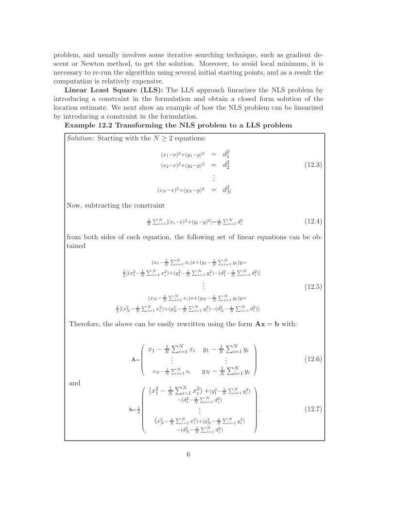
Linear Least Square (LLS): The LLS approach linearizes the NLS problem byintroducing a constraint in the formulation and obtain a closed form solution of thelocation estimate. We next show an example of how the NLS problem can be linearizedby introducing a constraint in the formulation.
Example 12.2 Transforming the NLS problem to a LLS problem
Solution: Starting with the N ≥ 2 equations:
(x1−x)2+(y1−y)2 = d21
(x2−x)2+(y2−y)2 = d22 (12.3)
...
(xN−x)2+(yN−y)2 = d2N
Now, subtracting the constraint
1N
∑Ni=1[(xi−x)2+(yi−y)2]= 1
N
∑Ni=1 d2
i (12.4)
from both sides of each equation, the following set of linear equations can be ob-tained
(x1−1N
∑Ni=1 xi)x+(y1−
1N
∑Ni=1 yi)y=
12[(x2
1−1N
∑Ni=1 x2
i )+(y21−
1N
∑Ni=1 y2
i )−(d21−
1N
∑Ni=1 d2
i )]
... (12.5)
(xN−1N
∑Ni=1 xi)x+(yN−
1N
∑Ni=1 yi)y=
12[(x2
N−
1N
∑Ni=1 x2
i )+(y2N−
1N
∑Ni=1 y2
i )−(d2N−
1N
∑Ni=1 d2
i )].
Therefore, the above can be easily rewritten using the form Ax = b with:
A=
x1 −1N
∑Ni=1 xi y1 −
1N
∑Ni=1 yi
......
xN−1N
∑Ni=1 xi yN − 1
N
∑Ni=1 yi
(12.6)
and
b= 12
(x21 −
1N
∑Ni=1 x2
i ) +(y21−
1N
∑Ni=1 y2
i )
−(d21−
1N
∑Ni=1 d2
i )
...(x2
N−1N
∑Ni=1 x2
i )+(y2N−
1N
∑Ni=1 y2
i )
−(d2N−
1N
∑Ni=1 d2
i )
. (12.7)
6
Note that A is described by the coordinates of anchors only, while b is representedby the distances to the landmarks together with the coordinates of landmarks. Thus, theestimated location of wireless device using linear least squares is: x = (ATA)−1ATb.Due to the subtraction, the solution obtained from the linear equations (12.7) is notexactly the same as the solution of the original nonlinear equation (12.2). The calculationof the linear equations solution requires low computational power and the obtainedsolution can serve as the starting point for the nonlinear least squares problem. Ingeneral, nonlinear searching from the linear estimate produces more accurate resultsthan the linear method at the price of a higher computational complexity.
12.2.3 Classification via Machine Learning
The fingerprinting matching proposed in [3] can be viewed as a machine learning classi-fication method. In [3], a K -nearest neighbors (K -NN) method is used for positioningwireless device based on the closest known locations (i.e., training points) in the pre-constructed signal map. Thus, in the K -nearest neighbors method, the location estima-tion of the wireless device is assigned as the average location of its K nearest locationsin the signal map. If K = 1, then the position estimate of the wireless device is simplyassigned as the location of its nearest known location in the signal map.
In particular, this kind of localization process through matching includes two phases:off-line training phase, which is used to collect the training data for constructing a radiomap, and on-line localization phase, which is used to estimate the position of the wirelessdevice based on the pre-built radio map.
During the off-line phase, a mobile transmitter travels to known positions and broad-casts beacons periodically, and the RSS readings at each known position are measuredat the set of anchors. The RSS readings together with the locations where the RSSreadings are collected are called RF fingerprints, i.e. {(xj , yj), ss1, ss2, ..., ssN}, where(xj , yj), with j = 1, 2, ...,m, is the location of the mobile transmitter traveling andssi(xj , yj) with i = 1, 2, ..., N , is the RSS readings at the ith anchor. To mitigate theeffect of noise, each ssi is either the averaged value or the median value of multiplemeasurements collected over a time period. Collecting together the RSS readings fromm different locations from a set of N anchors provides a radio map.
During the online localization phase, localization is performed by measuring thetargeted wireless device’s RSS at each anchor, and the vector of RSS values - a fingerprint,i.e. {ss′1, ss
′
2, ..., ss′
N} is compared to the pre-built radio map. In the nearest neighborsmethod, the record in the radio map whose signal strength vector is the closest in theEuclidean sense to the observed RSS fingerprint is declared to correspond to the locationof the transmitter:
(x, y) = arg min(xj ,yj)
√
√
√
√
N∑
i=1
(ss′i − ssi(xj , yj))2 (12.8)
Other versions of this approach return the average position (e.g., centroid) of the top Kclosest vectors; i.e., K -nearest neighbors (K -NN). For example, if K = 2, it takes the
7
closest two candidates and returns the mid-point between them. Other techniques fromthe field of machine learning classification that have been used for indoor localizationinclude neural networks [15,16], decision trees [17,18] and support vector machines [19,20]. A disadvantage of this approach is that it requires a large number of training pointsto perform adequately and is labor intensive.
To reduce the training efforts, one approach is to use an Interpolated Map Grid (IMG)is used to build signal maps [4]. Since the quality of the signal map is sensitive to thenumber of known locations [21], the purpose of using an IMG is to improve the resolutionof the signal map so as to obtain better localization accuracy. Directly measuring theRSS at a large number of known locations is expensive, the purpose of the interpolationapproach is to improve the quality of the signal map based on the averaged RSS readingsfrom a smaller number of known locations. We next show an example on how to buildan IMG from the collected fingerprints.
Example 12.3 Building an IMG signal map
Solution: The area of interest is divided into a regular grid of equal sized tiles. Thecenter of the tile is representative of its location. The tiles are a simple way to mapthe expected signal strength to locations. Building an IMG is thus similar to ”surfacefitting”; the goal is to derive an expected fingerprint for each tile from the collectedfingerprints. There are several approaches in the literature for interpolating surfaces,such as splines and triangle-based linear interpolation. For instance, triangle-basedlinear interpolation, which divides the floor into triangular regions using a Delaunaytriangulation [4], can be used in IMG. The expected signal strength at the center ofeach grid can be linearly interpolated.
When performing localization, given the observed RSS readings of a targeting wirelessdevice, Gridded-RADAR uses IMG to build the signal map and returns the (x, y) of thenearest neighbor in the IMG as the one to localize.
12.2.4 Probabilistic Approaches
We next examine the probabilistic approaches, where the RSS is treated as a randomvariable that can be modeled as a log-normal distribution at a physical location [8],one category of probabilistic methods is maximum likelihood estimation (MLE) [22,23].Assuming the targeted wireless device is located at location Lj = (xj , yj), given theonline observed RSS values s, i.e. s = {ss′1, ss
′
2, ..., ss′
N}, the estimated location of thetargeted wireless device based on the MLE is given by:
(x, y) = arg maxLj
{p(Lj |s)}, (12.9)
where p(Lj|s) denotes the probability that the wireless device is at location Lj.Using Bayes’ rule, the above equation is equivalent to finding the position Lj which
maximizes
P (Lj|s) =P (s|Lj) × P (Lj)
P (s). (12.10)
8
Without a priori information about the position of the wireless device, we can assumethat the probabilities that the wireless device located at different places are equally likely.Therefore, the equation (12.10) can be rewritten as:
P (Lj |s) = c × P (s|Lj), (12.11)
where c = P (Lj)/P (s) is a constant.Equation (12.11) can be further simplified by assuming conditional independence of
the measurement from all anchors:
P (s|Lj) = P (ss′1|Lj) · P (ss′2|Lj) · · ·P (ss′N |Lj). (12.12)
Assuming the RSS measurements at each location follow a log-normal distribution, theexpected RSS vector at each location, i.e. ssi(xj, yj), P (s|Lj) for every location Lj canbe computed. Finally, the MLE returns the location Lj which maximizes P (s|Lj).
Rather than returning a single location, the position estimate can instead be given asan area of confidence. For example, the area-based probability (ABP) method [4] triesto return an area bounded by a pre-defined probability level that the wireless deviceis within the returned area. In this approach, the pre-defined probability is called theconfidence level, which is an adjustable parameter, and is represented by the parameterα. In the ABP method, it first divides the whole area of interest into a set of tiles.The RSS vector of each tile is represented by the expected RSS vector at the centerof each. This can be done by using one of the aforementioned interpolation methodssuch as linear interpolation. Given that the wireless device must be located within thearea of interest, i.e.
∑mj=1 P (Lj |s) = 1, ABP returns the top probability tiles up to its
confidence, α.
12.2.5 Statistical Supervised Learning Techniques
The statistical supervised learning method infers a function from supervised trainingdata. A localization algorithm that utilizes statistical supervised learning analyzes thetraining data and produces an inferred function that predicts the location of a wirelessdevice based on the input RSS vector. We next introduce Bayesian Networks as anexample of localization algorithms that employ statistical supervised learning.
Bayesian networks, also called belief networks or probabilistic networks are graphicalmodels for representing the interaction between variables visually. A Bayesian networkis composed of nodes and arcs between the nodes. Each node corresponds to a randomvariable, v, and has a value corresponding to the probability of the random variable,P (v). If there is a directed arc from node v to node w, this indicates that v has a directinfluence on w. This influence is specified by the conditional probability P (w|v). Thenetwork is a directed acyclic graph (DAG), namely, there are no cycles. The nodes andthe arcs between the nodes define the structure of the networks, and the conditionalprobabilities are the parameters given the structure.
Adopting a Bayesian Network (BN) for RSS based localization [7], BN encodes thesignal-to-distance propagation model into the Bayesian Graphical Model for locationestimation. In DAG, the parents of a vertex v, pa(v), are those vertices from which
point into v. The descendants of a vertex v are the vertices which are reachable from valong a direct path. A vertex w is called a child of v if there is an edge from v to w. Theparent(s) of v are taken to be the only nodes which have direct influence on v, so that vis independent of its non-descendant given its parents. In BN, the overall joint densityof v ∈ V , where v is a random variable, only depends on the parents of v, denoted pa(v):
p(V ) =∏
v∈V
p(vi|pa(vi)). (12.13)
Once p(V ) is computed, the marginal distribution of any subset of the variables of thenetwork can be obtained as it is proportional to overall joint distribution.
Figure 12.1 presents two Bayesian Network algorithms, M1 and M2. Each rectangleis a plate, and shows a part of the network that is replicated; the nodes on each plateare repeated for each of the N anchors whose locations are known. The vertices Xand Y represent location; the vertex si is the signal reading from the ith anchor; andthe vertex Di represents the Euclidean distance between the location specified by Xand Y and the ith anchor. The value of si follows should a signal propagation modelsi = b0i + b1i log Di, where b0i, b1i are the parameters specific to the ith anchor. Thedistance Di =
√
(X − xi)2 + (Y − yi)2 in turn depends on the location (X,Y ) of themeasured signal and the coordinates (xi, yi) of the ith anchor. The network models noiseand outliers by modeling the si as a Gaussian distribution around the above propagationmodel, with variance τi:
si ∼ N(b0i + b1i log Di, τi). (12.14)
The initial parameters (b0i, b1i, τi) of the model are unknown, and the training data
10
is used to adjust the specific parameters of the model according to the relationshipsencoded in the network. Through Markov Chain Monte Carlo (MCMC) simulation,the BN returns the sampled distribution of the possible location of X and Y as thelocalization result.
The M1 model utilizes a simple Bayesian Network model, as depicted in Figure 12.1(a),and requires location information in the training set in order to give good localizationresults. The M2 model extends this to a hierarchical model as shown in Figure 12.1(b),which makes the coefficients of the signal propagation model have common parents.The BN M2 algorithm can localize multiple devices simultaneously with no trainingset, which can significantly reduce the labor-intensive efforts of training data collectionduring location estimation.
12.2.6 Summary of Localization Algorithms
We summarize RSS-based localization approaches and their main characteristics in Ta-ble 12.1. Compared to the other methods, lateration based approaches are sensitive toRSS noise caused by environmental bias, e.g., multipath effects. On the other hand, themachine learning classification and probabilistic approaches are robust to environmentalbias and RSS noise. However, they either need to collect a large number of trainingdata to build RSS profiles and is thus labor intensive, or require prior knowledge of RSSdistributions. Concerning localization using statistical supervised learning, it has theadvantage of being able to localizing multiple devices at the same time; and can returnreasonable localization accuracy even without training.
12.3 Localization Performance Study
The performance of each of the localization techniques needs to be evaluated throughvarious aspects. In this section, we first outline the main evaluation metrics and thenpresent a performance comparison across different localization algorithms using WiFiand ZigBee networks.
12.3.1 Performance Metrics
The set of evaluation metrics that we overview includes: accuracy, precision, robustness,complexity, and stability.
Accuracy. For a given localization attempt, accuracy is the Euclidean distancebetween the location estimate obtained from the localization system and the actual lo-cation of the targeted wireless device in the physical space. Accuracy is also referredto as localization error or distance error. Usually, the average or median distance erroris adopted as the performance metric. The better the accuracy, the better the loca-tion technique. Thus, accuracy can be used to evaluate the overall performance of thelocalization techniques.
Precision. Precision is defined as the success probability of position estimationswith respect to the predefined accuracy. Precision details the statistical characterization
11
Table 12.1: Summary of RSS-based localization approaches and their main characteris-tics.
Approach Description Algorithm
Example
Lateration - Two steps are involved: ranging andlateration. During ranging, the distancesbetween the wireless device and multipleanchors can be derived according to differentmeasurement modality. RSS is one of theapproaches to be used for ranging. Duringlateration, the location of the wireless devicecan be estimated according to derived dis-tances based on least squares methods.- Pros: This method is simple to use andworks well in free-space.- Cons: This method is sensitive to RSSvariation, e.g., multipath effects.
- It builds a priori radio signal map of thelocalization region during the training phasebased on the measured signal strength (i.e.RSS fingerprints) at different locations. Dur-ing localization, by comparing the onlinemeasured RSS to the pre-constructed signalmap, the location can be deduced.- Pros: This approach is robust to RSS noiseand environmental bias, e.g., multipath ef-fects;- Cons: It is labor intensive to build signalmap.
- The RSS is treated as a random variable bymodeling it with a log-normal distribution ateach location. The position of the wirelessdevice is returned as the most likely locationwith highest probability.- Pros: This approach is robust to RSSnoise and environmental bias, given the prioriknowledge of RSS distribution at large num-ber of locations.- Cons: It needs to use the RSS-distributionas priori knowledge, e.g., obtain RSS-distribution through training.
MaximumLikelihoodEstimation
StatisticalSupervisedLearning
- This approach derives the sample distribu-tion of the estimation locations based on sta-tistical learning.- Pros: This approach has the capability oflocalizing multiple devices at the same time;and returns reasonable localization accuracyeven without training data.- Cons: It can be computational intensive.
BayesianNetwork
12
of the localization error, which varies over many localization trials. It measures howconsistently the localization technique works and reveals the variation of localizationerrors. In some works, precision is defined as the standard deviation of the localizationerror or the geometric dilution of precision (GDOP) [24, 25]. However, generally theCumulative Distribution Function (CDF) of the localization error is used for measuringthe precision of an indoor localization system. When the accuracies of two locationalgorithms are the same, the algorithm which gives better precision is preferred. Inpractice, precision is described by either a CDF or the percentile format. For example,one typical indoor location system has a location precision of 97% within 30 feet (thelocalization error is less than 30 feet with probability of 97%), and median error as 10feet.
Robustness. A robust positioning should be able to function normally even whensome signals are not available, or when some of the RSS patterns haven’t been seen be-fore. For example, the signal at an anchor point may be blocked, thus the RSS reading atthat anchor point may be missing or incorrect. Sometimes, the environment changes, forexample due to furniture relocation, or the presence and mobility of human beings, willchange the RSS patterns. In addition, some anchors could be out of function or damagedin a harsh environment. For example, under malicious attacks, the attackers can con-trol anchor points and manipulate the RSS measurements. The positioning techniqueshave to use this incomplete information to localize the wireless devices. Therefore, it isimportant to measure the robustness of the localization algorithms. In all these cases, ifa localization technique is robust, then it should be able to provide the wireless device’sposition information without a reduced accuracy even if the quality of the measurementis reduced.
Complexity. Complexity of a localization system can be attributed to hardware,computing, and human intervention/efforts during deployment. The most commonlyused measure of complexity is the computing complexity, which is the complexity of thelocalization algorithm. If the computation of the localization algorithm is performed ina distributed manner (i.e., on the wireless device side), then we would prefer localiza-tion algorithms with low complexity, which can extend the operation life of the deviceswhich have the limited battery or power supply. Alternatively, we can use localizationlatency, the time it takes for a wireless device to localize. The first time and amortizedlatencies are different. For example, the first localization of a wireless device is long, butsubsequent localization attempts in nearby areas are typically much faster.
Stability. Stability measures how much the location estimate changes in the physicalspace in response to small-scale movements of a wireless device. Stability is a desirableproperty in localization systems, since a location estimate should not move too far inthe physical space if there is a small-scale movement of the wireless device. For instance,when someone works at his office desk and moves his laptop 1 feet away, the localizedposition of the laptop should not change too much.
13
(a) WINLAB (b) ORBIT room
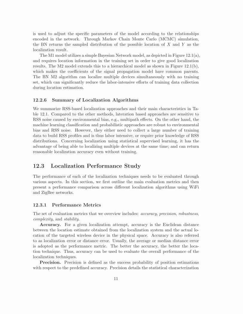
Figure 12.2: Deployment of anchors and training locations on the experimental floors [27,28].
12.3.2 Performance Investigation using Real Wireless Networks
We next compare the performance of different localization algorithms using WiFi andZigBee wireless networks by focusing on accuracy and precision. We first describe theexperimental scenarios in real office building environments. We then examine the exper-imental results across localization algorithms under different experimental scenarios.
Experimental Scenarios. Figure 12.2 shows two experimental scenarios for lo-calization performance comparison. The floor map in Figure 12.2(a) is the WirelessNetwork Laboratory (WINLAB) at Rutgers University, which has the floor size of 219ftby 169ft. Both a WiFi network and a ZigBee network are deployed in WINLAB. TheZigBee network is implemented using Tmote Sky motes. The second experimental setupshown in Figure 12.2(b) is the ORBIT testbed in WINLAB [26], a large scale indoorwireless testbed, which consists of 400 wireless nodes in a 20 × 20 regular grid with aninter-node separation of 3ft spanning a total area of 3600 sq ft. The WiFi network isused in the ORBIT testbed.
The distinctive characteristic between these two experimental scenarios are the num-ber of anchor points and the propagation environments. In the WINLAB office setup, it isa typical indoor propagation environment with heavy multipath effects due to the walls,furniture and people movement. There are 5 anchors shown as stars in Figure 12.2(a)and denoted as A, B, C, D, and E. On the other hand, in the ORBIT testbed, therecan be up to 400 anchor points and the propagation environment is free of major shad-owing and with limited multipath effects. Each wireless node in Figure 12.2(b) can beconfigured as an anchor point.
Furthermore, the small dots in Figure 12.2(a) are the training points where the RSSreadings are collected at each anchor. There are total 101 training locations in WINLABsetup. On the other hand, in the ORBIT testbed, the RSS readings are measured at eachgrid point. Thus, there are total 400 training locations in the ORBIT testbed. At eachlocation, about 350 packets of RSS are collected and the averaged RSS for each location
14
Table 12.2: Performance Study: Localization algorithms used in WINLAB environment.Algorithm Abbr. Description
Non-linear Least Squares NLS Lateration based algorithm,Non-linear Least Squares are used
Linear Least Squares LLS Lateration based algorithm,Linear Least Squares are used
Fingerprinting Matching RADAR Classification based method,Returns the nearest neighbor: K = 1
Area Based Probability ABP Probabilistic method using IMG,Returns the most likely area: α = 0.75Tile size in IMG: 10inch x 5 inch
Figure 12.3: Performance comparison: localization error CDF across different algorithmsunder the WINALB experimental scenario [27].
is used. To evaluate the different algorithms, the well-known leave-one-out approach isused to divide the data into training and testing sets. That means one location is chosenas the targeted location whereas the rest of the locations as training data. For example,in the lateration based algorithm, one location is randomly chosen to be localized andthe rest of the data (i.e., training data) are used to fit the propagation model (e.g.,equation 12.1) to get the propagation parameters, such as path loss parameters.
Performance Results. The algorithms under evaluation in the WINLAB officeexperimental scenario are: NLS, LLS, RADAR, ABP, and BN. These algorithms aresummarized in Table 12.2.
We note that when using ABP, because it returns the most likely area in whichthe targeted wireless device may reside, the localization error is defined as the medianlocalization error from the returned area.
The localization results in both WiFi network and ZigBee network are depicted asthe Cumulative Distribution Function (CDF) of localization error in Figure 12.3. Weobserved that the overall performance of localization algorithms under the WiFi network
15
Table 12.3: Performance Study: Localization algorithms used in ORBIT testbed.Algorithm Abbr. Description
Non-linear Least Squares NLS Lateration based algorithmNon-linear Least Squares are used
Fingerprinting Matching GR Classification based method using IMGGridded RADAR Returns the nearest neighbor: K = 1
tile size in IMG: 2inch x 2inchHighest Probability H1 Probabilistic method using IMG
Returns location with the highest probabilitytile size in IMG: 2inch x 2 inch
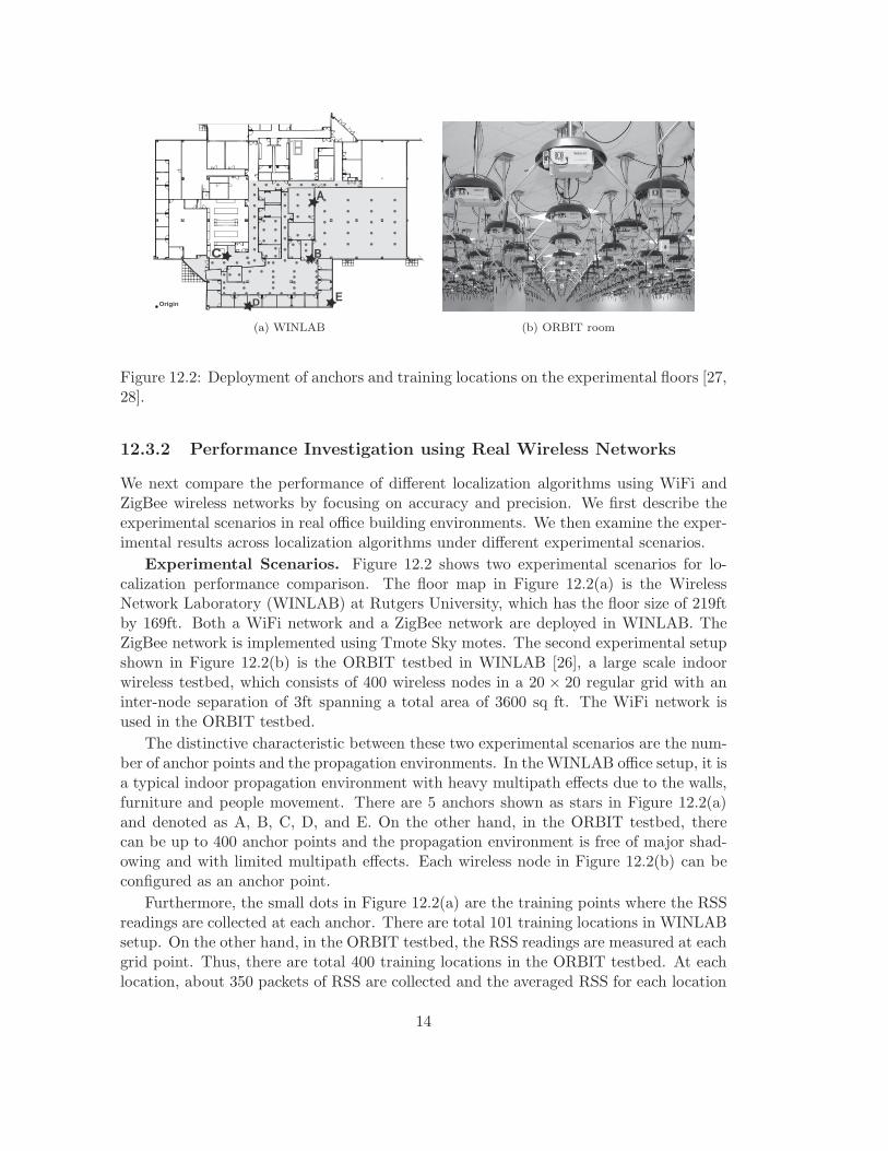
Figure 12.4: Performance comparison: localization error CDF across different algorithmsunder the ORBIT testbed experimental scenario [28].
is better than that of the Zigbee network due to the fact that WiFi device is morereliable than motes [27]. First, the median error from different algorithms ranges from7 feet to 20 feet in the WiFi network, whereas it is from 8 feet to 30 feet in the Zigbeenetwork. For both networks, ABP performs the best because it uses a fine-grainedsignal map via the IMG technique, while lateration based method performs the worstbecause of the inaccurate ranging information derived from the RSS readings affectedby the unpredictable indoor setups. In addition, RADAR and BN have comparableperformance in both networks. The median error is about 10 feet in the WiFi networkand 20 feet in Zigbee network, respectively.
We now turn to study the algorithms under evaluation in the ORBIT testbed. Thealgorithms under study are summarized in Table 12.3. Figure 12.4 shows the localizationerror CDF across different algorithms using the ORBIT testbed with 400 anchors [28].With the high density of anchors and benign propagation which is essentially LOS, theperformance of all the algorithms improves significantly. Again, the algorithms usingIMG have the best performance, while the lateration based method underperforms theother algorithms. Particularly, Gridded RADAR (GR) and Highest Probability (H1)have the best performance with median errors of 0.31 m and 0.33 m, respectively. Using
16
Bayesian Networks (M1) performs slightly worse, with the median error at 0.58 m. NLSperforms the worst with median error of about 2 meters. This is because the laterationalgorithms generally are very sensitive to data from low-quality anchors among the largenumber of anchors that cannot be fitted in the propagation model [28].
From the results in these two experimental scenarios, the following important con-clusions can be drawn:
1. The IMG technique can improve the localization accuracy of RADAR, ABP, andBN localization algorithms, because it provides a fine-grained signal map thatbenefits these algorithms.
2. The lateration based method is sensitive to the RSS variations caused by multi-patheffects, radio interference or the off-the-shelf device diversity, and have the worstlocalization performance. This is because the theoretical propagation model eithercannot describe complicated indoor environments (e.g., multipath effect) or need tobe calibrated due to device diversity (e.g., different transmitting power level), andthus the ranging information derived from RSS together with propagation modelis inaccurate.
3. Except the lateration based methods, all the other localization strategies, such asfingerprinting matching, probabilistic, and statistic learning, can achieve compa-rable localization accuracy and precision in a typical indoor environment.
4. Finally, a benign propagation environment or increasing the density of high-qualityanchors can improve the localization performance significantly.
12.4 Enhancing the Robustness of Localization
We next provide an overview of the methods that help to enhance the robustness of thelocalization results. These methods are either specific to one category of localizationalgorithms, (e.g., robust statistical methods can be applied to lateration techniques andfingerprinting matching methods, and revisiting linear regression and correlation meth-ods are suitable for lateration methods) or generic to all the localization algorithms, forinstance, employing multiple antennas to improve localization accuracy.
12.4.1 Real-time Infrastructure Calibration
In an indoor environment, radio signal propagation is affected by several factors such asmulti-path effects, environmental temperature and humidity variations, door’s openingand closing, and the mobility of human beings. The RSS readings at a given locationwill be very different over time since the indoor environment will change from time totime. To overcome the degradation of the localization performance due to environmentalchanges, it is necessary to calibrate the parameters of the positioning system, such as thepropagation parameters and signal maps. However, collecting RSS readings to calibratethe localization system from time to time manually is labor intensive. For example,collecting RSS readings at different locations to update the signal map periodically to
17
Anchor 2Anchor 3
Anchor 1
Anchor 4
Anchor 5
<Signal d>
<Signal d>
<Signal d>
<Signal d>
<Signal d>
<Signal d>
<Signal d>
<Signal d>
<Signal ?> <Signal ?>
<Signal ?>
<Signal ?>
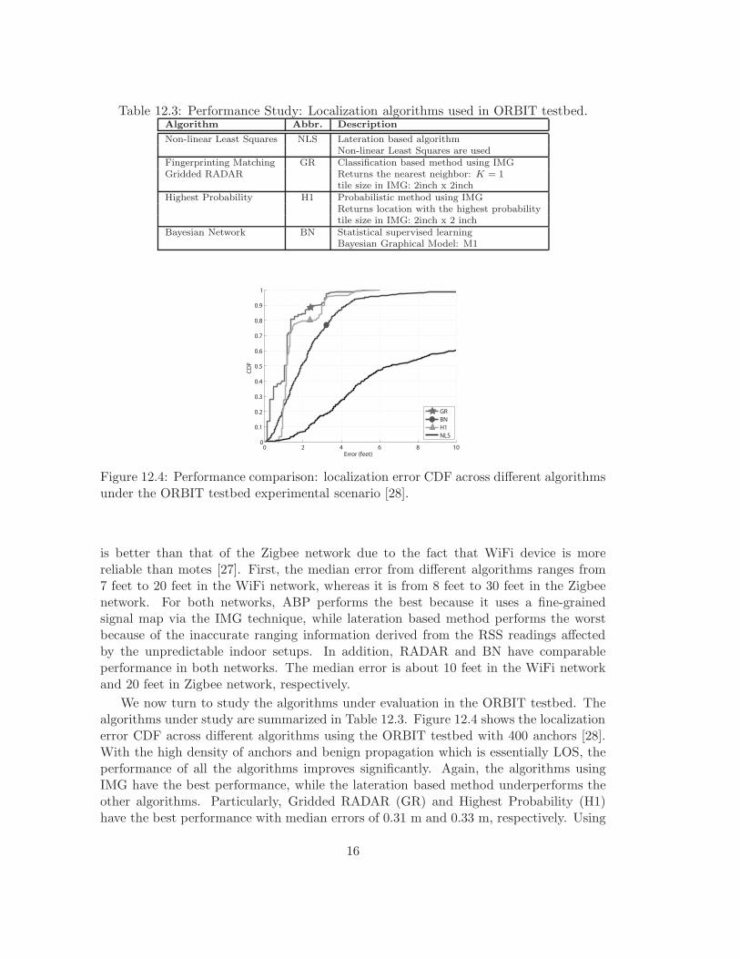
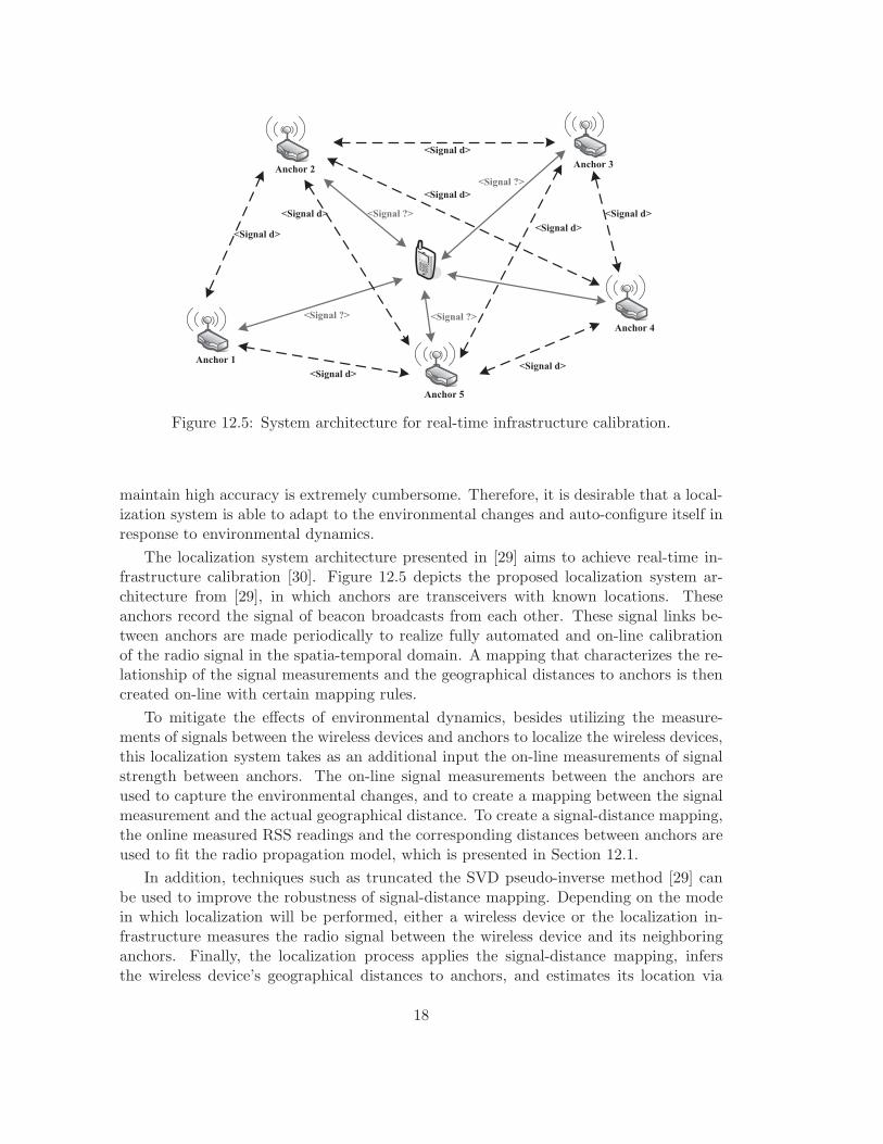
Figure 12.5: System architecture for real-time infrastructure calibration.
maintain high accuracy is extremely cumbersome. Therefore, it is desirable that a local-ization system is able to adapt to the environmental changes and auto-configure itself inresponse to environmental dynamics.
The localization system architecture presented in [29] aims to achieve real-time in-frastructure calibration [30]. Figure 12.5 depicts the proposed localization system ar-chitecture from [29], in which anchors are transceivers with known locations. Theseanchors record the signal of beacon broadcasts from each other. These signal links be-tween anchors are made periodically to realize fully automated and on-line calibrationof the radio signal in the spatia-temporal domain. A mapping that characterizes the re-lationship of the signal measurements and the geographical distances to anchors is thencreated on-line with certain mapping rules.
To mitigate the effects of environmental dynamics, besides utilizing the measure-ments of signals between the wireless devices and anchors to localize the wireless devices,this localization system takes as an additional input the on-line measurements of signalstrength between anchors. The on-line signal measurements between the anchors areused to capture the environmental changes, and to create a mapping between the signalmeasurement and the actual geographical distance. To create a signal-distance mapping,the online measured RSS readings and the corresponding distances between anchors areused to fit the radio propagation model, which is presented in Section 12.1.
In addition, techniques such as truncated the SVD pseudo-inverse method [29] canbe used to improve the robustness of signal-distance mapping. Depending on the modein which localization will be performed, either a wireless device or the localization in-frastructure measures the radio signal between the wireless device and its neighboringanchors. Finally, the localization process applies the signal-distance mapping, infersthe wireless device’s geographical distances to anchors, and estimates its location via
18
0 10 20 30 40 50 600
0.2
0.4
0.6
0.8
1
Error (feet)
Pro
ba
bil
ity
1−antenna
2−antenna−noavg
2−antenna−avg
2−antenna−avg−plus−1
3−antenna−noavg
3−antenna−avg
3−antenna−avg
1−antenna
0 10 20 30 40 50 600
0.2
0.4
0.6
0.8
1
Error (feet)
Pro
ba
bil
ity
1−antenna
2−antenna−noavg
2−antenna−avg
2−antenna−avg−plus−1
3−antenna−noavg
3−antenna−avg
1−antenna
3−antenna−noavg
(a) RADAR (b) ABP
0 20 40 60 80 1000
0.2
0.4
0.6
0.8
1
Error (feet)
Pro
bab
ilit
y
1−antenna
2−antenna−noavg
2−antenna−avg
2−antenna−avg−plus−1
3−antenna−noavg
3−antenna−avg
3−antenna−noavg
1−antenna
0 20 40 60 80 1000
0.2
0.4
0.6
0.8
1
Error (feet)
Pro
bab
ilit
y
1−antenna
2−antenna−noavg
2−antenna−avg
2−antenna−avg−plus−1
3−antenna−noavg
3−antenna−avg
3−antenna−noavg
1−antenna
(c) Bayesian Network: M1 (d) Bayesian Network: M2
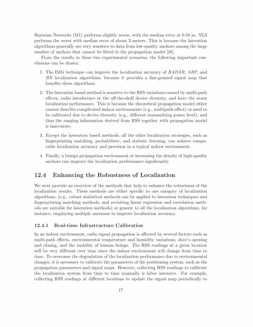
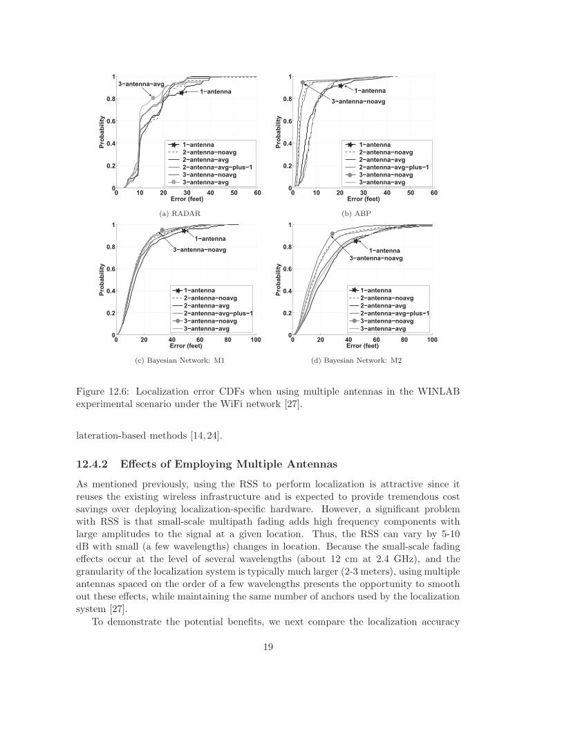
Figure 12.6: Localization error CDFs when using multiple antennas in the WINLABexperimental scenario under the WiFi network [27].
lateration-based methods [14,24].
12.4.2 Effects of Employing Multiple Antennas
As mentioned previously, using the RSS to perform localization is attractive since itreuses the existing wireless infrastructure and is expected to provide tremendous costsavings over deploying localization-specific hardware. However, a significant problemwith RSS is that small-scale multipath fading adds high frequency components withlarge amplitudes to the signal at a given location. Thus, the RSS can vary by 5-10dB with small (a few wavelengths) changes in location. Because the small-scale fadingeffects occur at the level of several wavelengths (about 12 cm at 2.4 GHz), and thegranularity of the localization system is typically much larger (2-3 meters), using multipleantennas spaced on the order of a few wavelengths presents the opportunity to smoothout these effects, while maintaining the same number of anchors used by the localizationsystem [27].
To demonstrate the potential benefits, we next compare the localization accuracy
19
across different localization algorithms when using multiple antennas [31]. Figure 12.6presents the localization error CDFs of different localization algorithms including RADAR,ABP, and Bayesian Networks when multiple antennas are applied. The experimentalscenario is the WINLAB environment under the WiFi network. The observation fromFigure 12.6 is that in nearly all cases the performance of localization algorithms improvedwhen using multiple antennas. This is because for RADAR, the collected training pointsare directly used to build the signal map. The distances of the training points in theexperiments range from 5ft to 10ft. The improvement for the RADAR algorithm comesfrom the reduced RSS variation when averaging RSS readings of three antennas. How-ever, for ABP, a fine-grained interpolated signal map is used, where the tile size is around10inch per side. When using the fine-grained interpolated signal map, the physical dis-tance between two RSS samples is much less (i.e. several inches) than the distancebetween two antennas (i.e. 1 to 2 ft in this experimental set) installed on one anchor.Thus, ABP treats each antenna as a separate anchor and achieves the best performanceunder the case of 3 − antenna− noavg.
In addition, Bayesian Networks present consistent behaviors when using differentBayesian Graphical Models (i.e. M1 and M2). The performance of 3− antenna−noavgis slightly better than that of others, and the 1 − antenna performs the worst. This isdue to the fact that Bayesian Networks benefit from the smoothed out small-scale fadingwhen averaging RSS readings of three antennas. In summary, we can conclude that thelocalization accuracy can be improved when employing multiple antennas in both casesof averaging and not averaging the RSS readings from multiple antennas at each anchorpoint.
12.4.3 Robust Statistical Methods
In indoor environment, signal strength measurements may be significantly altered byopening doorways in a hallway, or by the presence of passers by. These measurementerrors caused by either unintentional human behaviors or intentional adversarial behav-iors can be severe, and consequently degrade the performance of a localization method.On the other hand, these measurement errors may only be present on a small subsetof anchors (i.e., specific radio links between a wireless device and the affected anchors).The idea of the robust statistical method is to utilize the redundancy in the localizationinfrastructure, i.e., only a portion of the RSS readings at certain anchors is affectedand not all of the RSS readings are affected. The strategy is to enhance the robustnessof the localization system so as to mitigate the effects of such measurement errors andadversarial behaviors by taking advantage of the redundancy in the deployment of thelocalization infrastructure to provide stability to contaminated measurements [32].
Statistical tools are developed to make localization techniques robust to measurementerrors and adversarial data. In particular, the methods developed make use of the medianas a resilient estimate of the average of aggregated data [33,34]. For example, in laterationmethods, rather than minimizing the summation of the residue squares, minimizing themedian of the residue squares is used to reduce the effects of measurement outliers. Thelateration algorithm is vulnerable to the ”outliers”.
20
Given the distance from the wireless devices to the anchors di together with theanchors’ location (xi, yi), the device location estimate (x0, y0) can be found by leastsquares (i.e. equation (12.2)). In order to achieve accurate localization estimation whenthere are measurement errors present, LMS can be used instead of least squares. Thatis, (x0, y0) can be found such that
(x0, y0) = arg min(x0,y0)
medi[√
(xi − x0)2 + (yi − y0)2 − di]2. (12.15)
It is known that LMS tolerates up to 50 percent measurement errors among N totalmeasurements. The exact solution for LMS is computationally prohibitive, however, anefficient and statistically robust alternative can be found in [35].
12.4.4 Revisiting Linear Regression
Radio propagation indoors is complicated by signal reflection, refraction, shadowing andscattering due to the walls, furniture and the movement of people. According to theconnectivity between the wireless device and the anchor point, the signal propagationcan be classified into line-of-sight (LOS) and non-line-of-sight (NLOS) scenarios [3, 36].These two scenarios represent different signal propagation environments. Thus, underdifferent scenarios, the propagation parameters are different, such as the path loss expo-nent and the shadow fading as described in equation (12.1). The training data collectedin the area of interest usually includes both LOS and NLOS scenarios and we cannotdifferentiate which scenario the targeting wireless device belongs to. Thus, in the off linetraining phase, the fitted theoretical log-distance propagation model can not characterizeboth LOS and NLOS scenarios simultaneously and will result in large errors in distanceestimation during the ranging step of RSS-based lateration methods, and consequentlythe localization accuracy is significantly affected. In Section 12.3, we observed that RSS-based lateration methods underperform other indoor localization algorithms includingmachine learning classification techniques, probabilistic approaches, and Bayesian Net-work localization.
To improve the applicability of RSS-based lateration methods in indoor environmentsand further provide feasible mathematical analysis for indoor localization, a regressionmodel may be used over the theoretical log-distance propagation model to better modelthe relationship between the RSS and distance and improve localization accuracy forlateration methods in real-world scenarios [14].
The polynomial regression model is adapted to model the RSS to distance relationshipsince the polynomials dominate the interpolation theory (Weierstrass’s Theorem) andthey are easily evaluated [37].
Example 12.4 Using polynomial regression model to model the relation-ship between the RSS and distance
21
Solution: Given the M training points (di, RSSi) collected in the area of interest,where di is the distance between the wireless device and an anchor point and RSSi
is the corresponding signal strength reading at the training point i. The nth-degreepolynomial is fitted through the set of data and M sets of equations are obtained.The ideal nth-degree polynomial should satisfy:
di = a0 + a1 ∗ RSSi + a2 ∗ RSS2i + ... + an ∗ RSSn
i (12.16)
where aj (with j = 0, 1, 2, ..., n) are the coefficients of the polynomial, RSSi is
the received signal strength and di is the estimated distance. However, there areestimation errors ei. Thus, we have:
ei=(di−di)=(di−a0−a1∗RSSi−...−an∗RSSni ), (12.17)
where i = 1, 2, ...,M .We use least squares approximation, in which the coefficients can be obtained byminimizing the sum of the error squares, which is given by
E(a0, a1, ..., an) =
i=M∑
i=1
(ei)2 (12.18)
The equation (12.18) is a function of variables, a0, a1, ..., an, which minimizes thesum of error squares. We equate its partial derivatives to zero with respect toa0, a1, ..., an. Then, we get
∂E
∂aj
=∑i=M
i=1 −2(RSSji )(di−a0−a1∗RSSi−...−an∗RSSn
i )=0, (12.19)
for each j, with j = 0, 1, 2, ..., n. By rearranging equation (12.19), we obtain thenormal equations:
∑i=Mi=1 RSS
ji di=
a0∑i=M
i=1 RSSji +a1
∑i=Mi=1 RSS
(j+1)i +...+an
∑i=Mi=1 RSS
(j+n)i , (12.20)
for each j, with j = 0, 1, 2, ..., n. Now, the coefficients aj, with j = 0, 1, 2, ..., n, canbe solved by Gauss elimination of Equation (12.20).
Figure 12.7 presents the localization results of the regression-based methods using asecond degree of polynomial for both the WiFi network and the Zigbee network underthe WINLAB experimental scenario respectively. We observed that the regression-basedlateration methods result in a better performance than the original log-distance basedlateration methods. The overall improvement of median error is above 29% in both net-works. In addition, the maximum localization error is significantly reduced. The overallimprovement of maximum error is over 50% in two networks. These results indicate that
22
0 20 40 60 80 100 120 140 1600
0.1
0.2
0.3
0.4
0.5
0.6
0.7
0.8
0.9
1
Error (feet)
CD
F
LLS
NLS
Regression−based LLS
Regression−based NLS
0 20 40 60 80 100 120 140 1600
0.1
0.2
0.3
0.4
0.5
0.6
0.7
0.8
0.9
1
Error (feet)
CD
F
LLS
NLS
Regression−based LLS
Regression−based NLS
(a) WiFi network (b) Zigbee network
Figure 12.7: Regression-based approach: localization error CDFs in two networks [14].
using regression-based lateration methods are effective in indoor localization.
12.4.5 Exploiting Spatial Correlation
Although radio propagation is complicated due to the placement of walls, obstacles andmovement of people in indoors, the signal propagation from close-by locations in a localarea to an anchor point is highly correlated as nearby locations face a similar propagationenvironment. For instance, the locations in a regular-sized room are facing the sameradio connectivity to the access points (i.e., LOS or NLOS), and similar distance tothe anchor points. Thus, the signal propagation from a local area experiences similarsignal attenuation (due to distance) and penetration losses through walls. Therefore, thesignal propagation model may be better fitted if we just use the data collected in the localarea. Further, experimental results have provided strong evidence that shadow fadingis spatially correlated in indoors [38] due to the local area facing similar obstacles. Thecorrelation distance can range from several to many tens of meters [36, 38]. Therefore,the correlated RSS measurements collected in a local area can help to characterize therelationship between RSS and the distance, and consequently improve the localizationaccuracy when applying lateration methods in unpredictable indoor environments [14].
Example 12.5 Using spatial correlation to iteratively refine the localizationresults
The correlation-based method is developed in [14] by utilizing the correlated RSSreadings that are collected from a local area to fit the theoretical log-distance prop-agation model. The objective is to obtain more accurate distance estimations for thewireless device, whose location belongs to that local area, based on the fitted model. Thecorrelation-based method refines the localization result iteratively by using the correlatedRSS in the local area.
23
0 20 40 60 80 100 120 140 1600
0.1
0.2
0.3
0.4
0.5
0.6
0.7
0.8
0.9
1
Error (feet)
CD
F
LLS
NLS
Correlation−based LLS
Correlation−based NLS
0 20 40 60 80 100 120 140 1600
0.1
0.2
0.3
0.4
0.5
0.6
0.7
0.8
0.9
1
Error (feet)
CD
F
LLS
NLS
Correlation−based LLS
Correlation−based NLS
(a) WiFi network (b) Zigbee network
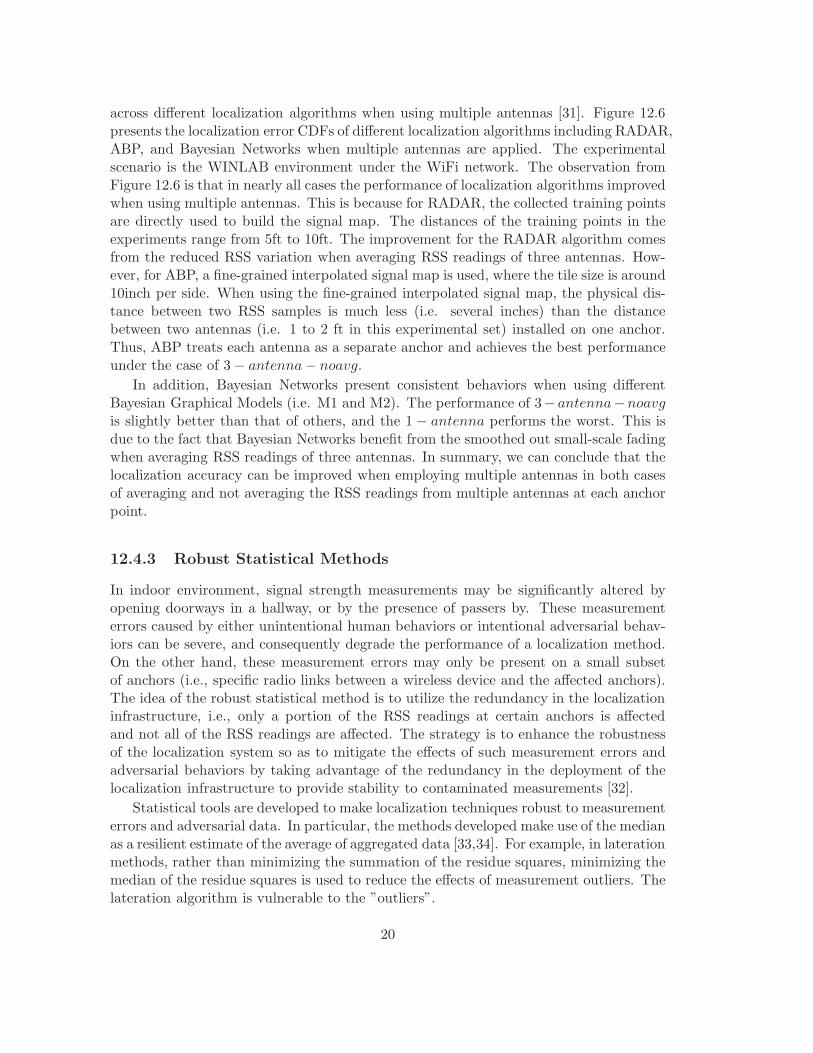
Figure 12.8: Correlation-based method: localization error CDFs in two networks [14].
Solution: The correlation-based method starts with a coarse-grained location es-timation by using lateration with all the training data. Then, in the subsequentiterative steps, it adaptively reduces the size of the training data by just using thedata that is close to the location estimate from the previous step. The iterativeprocess stops when the estimated location falls outside of the local area where thetraining data comes from. The correlation method is summarized as follows.
1. Initialize. Using all the training points (xj, yj) and corresponding RSS{RSSij} at multiple access points (xi, yi), with i = {1, 2, ...,M} and j ={1, 2, ..., N}, to fit the propagation model, and obtain the initial location(x0, y0) according to the measured RSS {RSSi} of the wireless device usingthe lateration method.
2. Iteration. Refine the wireless device’s location estimation (xk, yk), k is thekth iteration step, by using top Ck (Ck < Ck−1) closest training points to theprevious estimated location (xk−1, yk−1) as training data. Ck is the numberof training points used in kth iteration step.
3. Termination. Repeat step 2 until the refined location (xk, yk) falls outside ofthe area where the Ck training points come from. Return the wireless device’sfinal estimated location (x, y) = (xk−1, yk−1).
Figure 12.8 shows the localization error CDFs of correlation-based lateration methodsin the WiFi network and the Zigbee network under the WINLAB experimental scenariowhen the reducing rate of the training data size is set to 50%. The correlation-basedapproach significantly improves the accuracy of lateration methods in both median erroras well as maximum error. The overall improvement of median error is over 33% in both
24
networks.
12.5 Conclusion and Applications
In this chapter, we have provided an overview of RSS based localization approachesand algorithms for indoor localization. We focused in particular on the performance ofthese localization techniques and advanced techniques to enhance the robustness of thesealgorithms. Generally, the average localization accuracy of the RSS based localizationtechniques is around 10-20 feet. We compared the performance of these algorithmsin terms of accuracy and precision, and showed by experimental evaluations that thelocalization accuracy can be improved via several approaches, such as the interpolatedsignal map and increased density of anchors. Because the radio propagation in indoorsis complicated due to walls, furniture, and the movement of people, the robustness oflocalization algorithms is especially important in indoor environments. We thus describetechniques on enhancing the robustness of localization, in which the enhanced localizationtechniques are more robust to the environmental dynamics.
Location information can directly support a variety of location-based services or asinput to other high-level emerging pervasive applications. For example, in the healthcaredomain, doctors can directly use location information to track and monitor patients inmedical facilities, or activities can be inferred using the estimated position and higher-level decision can be made accordingly. In the latter case, if a doctor and a nurseare both localized in the same room as a patient, then it will be concluded that thispatient is getting treated. In the enterprise domain, location-based access control andasset tracking exploit location information directly. And the workflow management inindustrial plants needs the location information as lower level input for a specific task.
Future trends make it likely that wireless indoor positioning systems will be inte-grated into a unified localization infrastructure, which can provide spatial positioningof wireless devices across organizational boundaries, work with diverse technologies, andsupport numerous applications including social networking, manufacturing, retail andsecurity. Therefore, some important future research directions are: how to integrate thefragmented location systems belonging to different communities, such as indoor and out-door positioning systems; how to work with diverse technologies, such as different wirelessdevices (i.e., WiFi, Zigbee, Bluetooth, and mote sensors) and location techniques (i.e.,data fusion, hybrid location algorithms).
25
Bibliography
[1] P. Enge and P. Misra, Global Positioning System: Signals, Measurements and Per-formance. Ganga-Jamuna Pr, 2001.
[2] N. Priyantha, A. Chakraborty, and H. Balakrishnan, “The cricket location-supportsystem,” in Proceedings of the ACM International Conference on Mobile Computingand Networking (MobiCom), Aug 2000, pp. 32–43.
[3] P. Bahl and V. N. Padmanabhan, “RADAR: An in-building RF-based user loca-tion and tracking system,” in Proceedings of the IEEE International Conference onComputer Communications (INFOCOM), March 2000, pp. 775–784.
[4] E. Elnahrawy, X. Li, and R. P. Martin, “The limits of localization using signalstrength: A comparative study,” in Proceedings of the First IEEE InternationalConference on Sensor and Ad hoc Communcations and Networks (SECON 2004),Oct. 2004, pp. 406–414.
[5] Y. Chen, K. Kleisouris, X. Li, W. Trappe, and R. P. Martin, “A security and ro-bustness performance analysis of localization algorithms to signal strength attacks,”ACM Transactions on Sensor Networks (ACM TOSN), vol. 5, no. 1, February 2009.
[6] R. Battiti, M. Brunato, and A. Villani, “Statistical Learning Theory for LocationFingerprinting in Wireless LANs,” University of Trento, Informatica e Telecomuni-cazioni, Technical Report DIT-02-086, Oct. 2002.
[7] D. Madigan, E. Elnahrawy, R. Martin, W. Ju, P. Krishnan, and A. S. Krishnakumar,“Bayesian indoor positioning systems,” in Proceedings of the IEEE InternationalConference on Computer Communications (INFOCOM), March 2005, pp. 324–331.
[8] T. Rappaport, Wireless Communications: Principles and Practice. Prentice Hall,1996.
[9] T. Hastie, R. Tibshirani, and J. Friedman, “The elements of statistical learning:data mining, inference, and prediction. 2001,” NY Springer-Verlag.
[10] K. Langendoen and N. Reijers, “Distributed localization in wireless sensor networks:a quantitative comparison,” Comput. Networks, vol. 43, no. 4, pp. 499–518, 2003.
[11] D. Niculescu and B. Nath, “Ad hoc positioning system (APS),” in Proceedings of theIEEE Global Telecommunications Conference (GLOBECOM), 2001, pp. 2926–2931.
27
[12] J. Yang, Y. Chen, V. Lawrence, and V. Swaminathan, “Robust wireless localizationto attacks on access points,” in IEEE Sarnoff Symposium 2009, Princeton , NJ,USA.
[13] T. Sarkar, Z. Ji, K. Kim, A. Medouri, and M. Salazar-Palma, “A survey of var-ious propagation models for mobile communication,” Antennas and PropagationMagazine, IEEE, vol. 45, no. 3, pp. 51–82, June 2003.
[14] J. Yang and Y. Chen, “Indoor localization using improved rss-based lateration meth-ods,” in Proceedings of the IEEE Global Telecommunications Conference (GLOBE-COM), 2009.
[15] R. Battiti, R. Battiti, A. Villani, T. L. Nhat, T. L. Nhat, R. Villani, and R. Villani,“Location-aware computing: A neural network model for determining location inwireless lans,” Tech. Rep., 2002, tech. Rep.
[16] S.-H. Fang and T.-N. Lin, “Indoor location system based on discriminant-adaptiveneural network in ieee 802.11 environments,” Neural Networks, IEEE Transactionson, vol. 19, no. 11, pp. 1973 –1978, nov. 2008.
[17] Y. Chen, Q. Yang, J. Yin, and X. Chai, “Power-efficient access-point selection forindoor location estimation,” Knowledge and Data Engineering, IEEE Transactionson, vol. 18, no. 7, pp. 877 – 888, july 2006.
[18] J. Yim, “Introducing a decision tree-based indoor positioning technique,” ExpertSyst. Appl., vol. 34, no. 2, pp. 1296–1302, 2008.
[19] M. Brunato and R. Battiti, “Statistical learning theory for location fingerprintingin wireless ”lans”,” Comput. Netw., vol. 47, no. 6, pp. 825–845, 2005.
[20] C.-L. Wu, L.-C. Fu, and F.-L. Lian, “Wlan location determination in e-home viasupport vector classification,” in Networking, Sensing and Control, 2004 IEEE In-ternational Conference on, vol. 2, 2004, pp. 1026 – 1031 Vol.2.
[21] J. Yang and Y. Chen, “A theoretical analysis of wireless localization using RF-based fingerprint matching,” in Proceedings of the Fourth International Workshopon System Management Techniques, Processes, and Services (SMTPS), April 2008.
[22] M. Youssef, A. Agrawal, and A. U. Shankar, “WLAN location determination viaclustering and probability distributions,” in Proceedings of the First IEEE Interna-tional Conference on Pervasive Computing and Communications (PerCom), Mar.2003, pp. 143–150.
[23] M. Youssef and A. Agrawala, “Handling samples correlation in the horus system,”in IEEE Infocom, 2004, pp. 1023–1031.
[24] H. Lee, “A novel procedure for assessing the accuracy of hyperbolic multilaterationsystems,” Aerospace and Electronic Systems, IEEE Transactions on, vol. AES-11,no. 1, pp. 2 –15, jan. 1975.
28
[25] D. Torrieri, “Statistical theory of passive location systems,” Aerospace and Elec-tronic Systems, IEEE Transactions on, vol. AES-20, no. 2, pp. 183 –198, march1984.
[27] K. Kleisouris, Y. Chen, J. Yang, and R. P. Martin, “The impact of using multipleantennas on wireless localization,” in Proceedings of the Fifth Annual IEEE Com-munications Society Conference on Sensor, Mesh and Ad Hoc Communications andNetworks (SECON), June 2008.
[28] G. Chandrasekaran, M. Ergin, J. Yang, S. Liu, Y. Chen, M. Gruteser, and R. Martin,“Empirical evaluation of the limits on localization using signal strength,” in Sensor,Mesh and Ad Hoc Communications and Networks, 2009. SECON ’09. 6th AnnualIEEE Communications Society Conference on, 22-26 2009, pp. 1 –9.
[29] H. Lim, L. Kung, J. Hou, and H. Luo, “Zero-configuration, robust indoor local-ization: Theory and experimentation,” in Proceedings of the IEEE InternationalConference on Computer Communications (INFOCOM), March 2006.
[30] Y. Gwon and R. Jain, “Error characteristics and calibration-free techniques forwireless lan-based location estimation,” in MobiWac ’04: Proceedings of the secondinternational workshop on Mobility management & wireless access protocols. NewYork, NY, USA: ACM, 2004, pp. 2–9.
[31] K. Kleisouris, Y. Chen, J. Yang, and R. Martin, “Empirical evaluation of wirelesslocalization when using multiple antennas,” Parallel and Distributed Systems, IEEETransactions on, vol. PP, no. 99, 2010.
[32] Z. Li, W. Trappe, Y. Zhang, and B. Nath, “Robust Statistical Methods for SecuringWireless Localization in Sensor Networks,” in The Fourth International Conferenceon Information Processing in Sensor Networks (IPSN), 2005, pp. 91–98.
[33] B. Przydatek, D. Song, and A. Perrig, “”sia: Secure information aggregation insensor networks”,” in ACM SenSys, Nov. 2003.
[34] D. Wagner, “Resilient aggregation in sensor networks,” in Proceedings of the ForthACM Workshop on Security of Ad Hoc and Sensor Networks (SASN), 2004, pp.78–87.
[35] P. Rousseeuw and A. Leroy, Robust regression and outlier detection. John Wiley& Sons Inc, 1987.
[36] M. Gudmundson, “Correlation model for shadow fading in mobile radio systems,”Electronics Letters, vol. 27, pp. 2145–2146, 1991.
[37] J. L. Buchanan and P. R. Turner, Numerical Methods and Analysis. New York:McGraw-Hill, 1992.
29
[38] N. Jalden, P. Zetterberg, B. Ottersten, A. Hong, and R. Thoma, “Correlation prop-erties of large scale fading based on indoor measurements,” in Wireless Communi-cations and Networking Conference, 2007.WCNC 2007. IEEE, March 2007.