Chapter 13: Using the Mixing Plane Model · Fluid Flow and Heat Transfer in a Mixing Elbow ......

Chapter 13: Using the Mixing Plane Model

This tutorial is divided into the following sections:

13.1. Introduction

13.2. Prerequisites

13.3. Problem Description

13.4. Setup and Solution

13.5. Summary

13.6. Further Improvements

13.1. Introduction

This tutorial considers the flow in an axial fan with a rotor in front and stators (vanes) in the rear. This con-

figuration is typical of a single-stage axial flow turbomachine. By considering the rotor and stator together

in a single calculation, you can determine the interaction between these components.

This tutorial demonstrates how to do the following:

• Use the standard �

- �

model with standard wall functions.

• Use a mixing plane to model the rotor-stator interface.

• Calculate a solution using the pressure-based solver.

• Compute and display circumferential averages of total pressure on a surface.

13.2. Prerequisites

This tutorial is written with the assumption that you have completed Introduction to Using ANSYS FLUENT:

Fluid Flow and Heat Transfer in a Mixing Elbow (p. 111), and that you are familiar with the ANSYS FLUENT nav-

igation pane and menu structure. Some steps in the setup and solution procedure will not be shown explicitly.

13.3. Problem Description

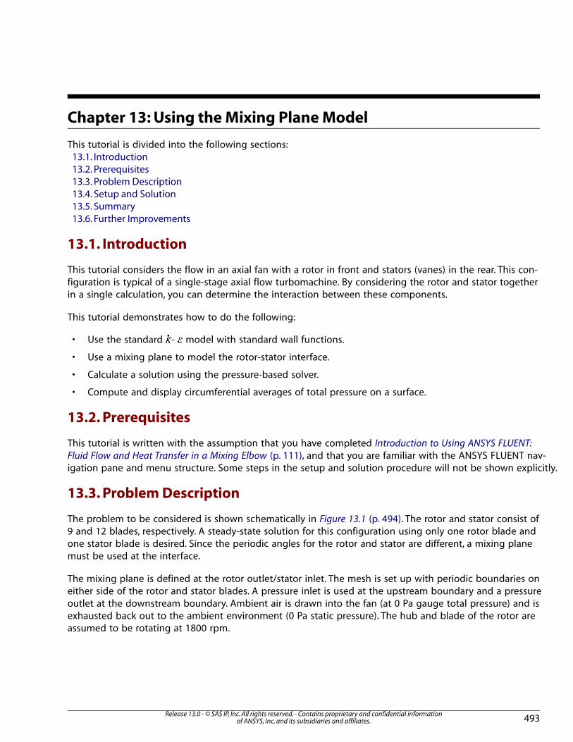
The problem to be considered is shown schematically in Figure 13.1 (p. 494). The rotor and stator consist of

9 and 12 blades, respectively. A steady-state solution for this configuration using only one rotor blade and

one stator blade is desired. Since the periodic angles for the rotor and stator are different, a mixing plane

must be used at the interface.

The mixing plane is defined at the rotor outlet/stator inlet. The mesh is set up with periodic boundaries on

either side of the rotor and stator blades. A pressure inlet is used at the upstream boundary and a pressure

outlet at the downstream boundary. Ambient air is drawn into the fan (at 0 Pa gauge total pressure) and is

exhausted back out to the ambient environment (0 Pa static pressure). The hub and blade of the rotor are

assumed to be rotating at 1800 rpm.

493Release 13.0 - © SAS IP, Inc. All rights reserved. - Contains proprietary and confidential information

of ANSYS, Inc. and its subsidiaries and affiliates.

Figure 13.1 Problem Specification

13.4. Setup and Solution

The following sections describe the setup and solution steps for this tutorial:

13.4.1. Preparation

13.4.2. Step 1: Mesh

13.4.3. Step 2: General Settings

13.4.4. Step 3: Models

13.4.5. Step 4: Mixing Plane

13.4.6. Step 5: Materials

13.4.7. Step 6: Cell Zone Conditions

13.4.8. Step 7: Boundary Conditions

13.4.9. Step 8: Solution

13.4.10. Step 9: Postprocessing

13.4.1. Preparation

1. Download mixing_plane.zip from the ANSYS Customer Portal or the User Services Center to your

working folder (as described in Preparation (p. 4) of Introduction to Using ANSYS FLUENT in ANSYS

Workbench: Fluid Flow and Heat Transfer in a Mixing Elbow (p. 1)).

2. Unzip mixing_plane.zip .

The file fanstage.msh can be found in the mixing_plane folder created after unzipping the file.

3. Use FLUENT Launcher to start the 3D version of ANSYS FLUENT.

For more information about FLUENT Launcher, see Starting ANSYS FLUENT Using FLUENT Launcher in

the User's Guide.

Note

The Display Options are enabled by default. Therefore, after you read in the mesh, it will be

displayed in the embedded graphics window.

13.4.2. Step 1: Mesh

1. Read the mesh file fanstage.msh .

File → Read → Mesh...

As ANSYS FLUENT reads the mesh file, it will report its progress in the console.

Release 13.0 - © SAS IP, Inc. All rights reserved. - Contains proprietary and confidential informationof ANSYS, Inc. and its subsidiaries and affiliates.494


http://www.ansys.com/customerportal/

http://www.fluentusers.com


General

1. Check the mesh.

General → Check

ANSYS FLUENT will perform various checks on the mesh and will report the progress in the console. Ensure

that the reported minimum volume is a positive number.

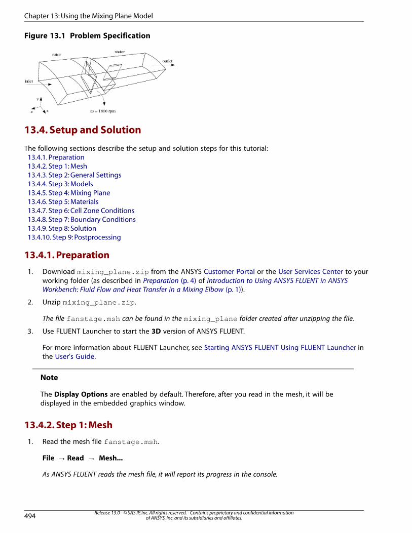
2. Display the mesh (Figure 13.2 (p. 496)).

General → Display...

a. Select only rotor-blade, rotor-hub, rotor-inlet-hub, stator-blade, and stator-hub from the

Surfaces selection list.

b. Click Display and close the Mesh Display dialog box.




Figure 13.2 Mesh Display for the Multistage Fan

Extra

You can use the right mouse button to check which zone number corresponds to each

boundary. If you click the right mouse button on one of the boundaries in the graphics

window, its zone number, name, and type will be printed in the ANSYS FLUENT console.

This feature is especially useful when you have several zones of the same type and you

want to distinguish between them quickly.

3. Retain the default solver settings.

General



4. Define new units for angular velocity.

General → Units...

The angular velocity for this problem is known in rpm, which is not the default unit for angular velocity.

You will need to redefine the angular velocity units as rpm.

a. Select angular-velocity from the Quantities selection list and rpm from the Units selection list.

b. Close the Set Units dialog box.


Models

1. Enable the standard �

- �

turbulence model with standard wall functions.




Models → Viscous → Edit...

a. Select k-epsilon (2eqn) in the Model list.

The Viscous Model dialog box will expand.

b. Retain the default selection of Standard in the k-epsilon Model list.

c. Retain the default selection of Standard Wall Functions in the Near-Wall Treatment list.

d. Click OK to close the Viscous Model dialog box.


Define → Mixing Planes...

In this step, you will create the mixing plane between the pressure outlet of the rotor and the pressure inlet of

the stator.



1. Select pressure-outlet-rotor from the Upstream Zone selection list.

2. Select pressure-inlet-stator from the Downstream Zone selection list.

3. Retain the selection of Area in the Averaging Method list.

4. Click Create and close the Mixing Planes dialog box.

ANSYS FLUENT will name the mixing plane by combining the names of the zones selected as the Upstream

Zone and Downstream Zone. This new name will be displayed in the Mixing Plane list.

The essential idea behind the mixing plane concept is that each fluid zone (stator and rotor) is solved as a

steady-state problem. At some prescribed iteration interval, the flow data at the mixing plane interface are

averaged in the circumferential direction on both the rotor outlet and the stator inlet boundaries. ANSYS

FLUENT uses these circumferential averages to define “profiles” of flow properties. These profiles are then

used to update boundary conditions along the two zones of the mixing plane interface.

In this example, profiles of averaged total pressure (��

), static pressure (��

), direction cosines of the local

flow angles in the radial, tangential, and axial directions (� � �� ), total temperature (

�), turbulent

kinetic energy (

), and turbulent dissipation rate (�

) are computed at the rotor exit and used to update

boundary conditions at the stator inlet. Likewise, the same profiles, except for that of total pressure are

computed at the stator inlet and used as a boundary condition on the rotor exit.

The default method for calculating mixing plane profiles uses an area-weighted averaging approach. This

method allows reasonable profiles of all variables to be created regarding of the mesh topology. In some

cases, a mass flow-weighted averaging may be appropriate (for example, with compressible turbomachinery

flows). For such cases, the Mass option can be enabled as shown. A third averaging approach (the Mixed-

Out average) is also available for flows with ideal gases. Refer to Choosing an Averaging Method of the

Theory Guide for more information on these averaging methods.

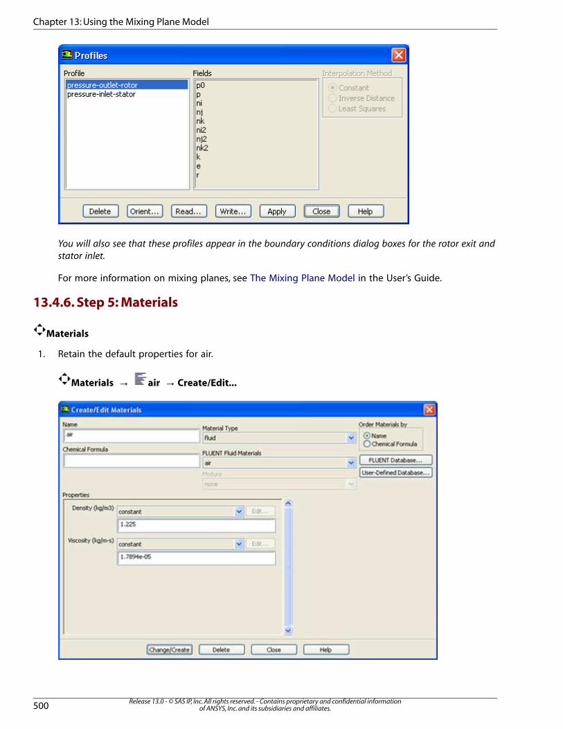
You can view the profiles computed at the rotor exit and stator inlet in the Profiles dialog box.

Define → Profiles...




You will also see that these profiles appear in the boundary conditions dialog boxes for the rotor exit and

stator inlet.

For more information on mixing planes, see The Mixing Plane Model in the User’s Guide.

13.4.6. Step 5: Materials

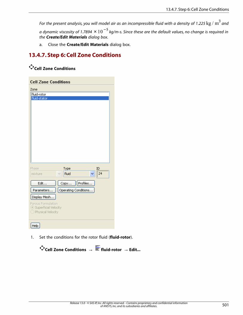
Materials

1. Retain the default properties for air.

Materials → air → Create/Edit...



For the present analysis, you will model air as an incompressible fluid with a density of 1.225

� and

a dynamic viscosity of 1.7894 × −� kg/m-s. Since these are the default values, no change is required in

the Create/Edit Materials dialog box.

a. Close the Create/Edit Materials dialog box.


Cell Zone Conditions

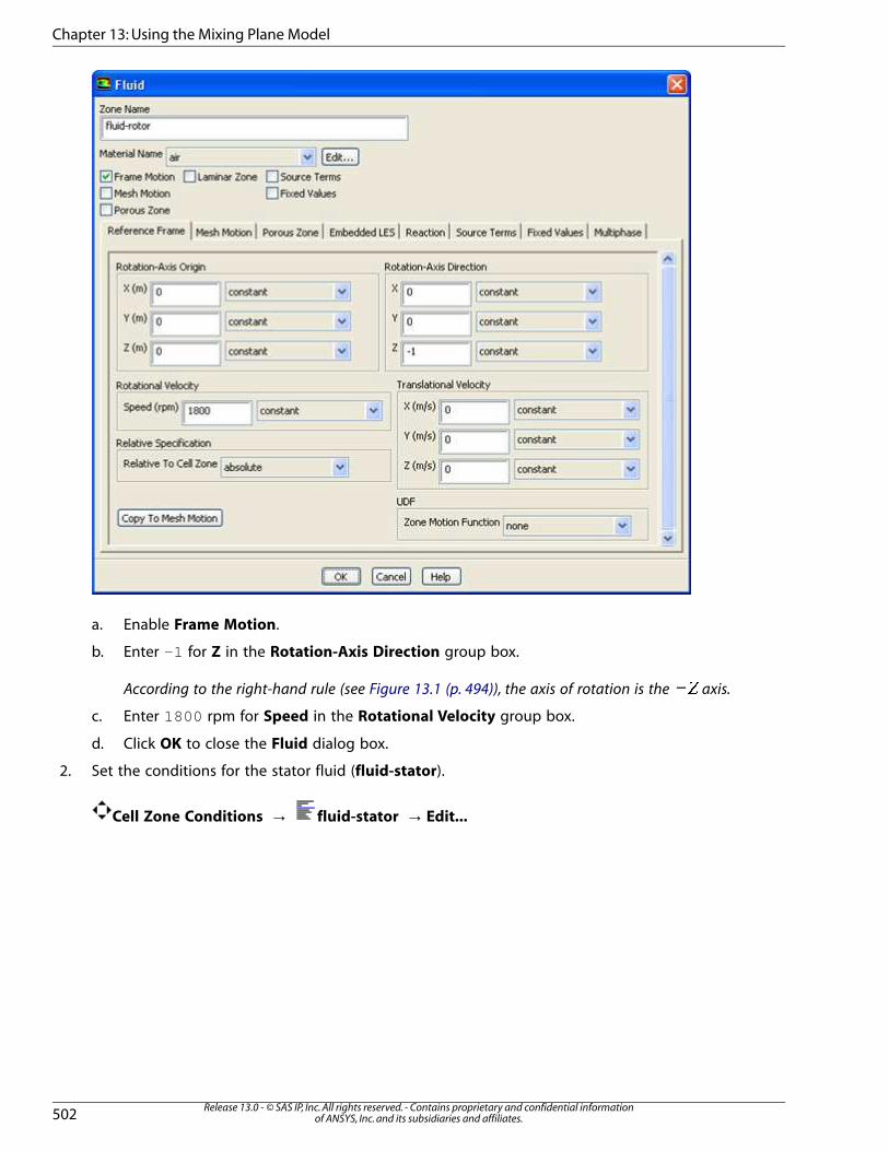
1. Set the conditions for the rotor fluid (fluid-rotor).

Cell Zone Conditions → fluid-rotor → Edit...




a. Enable Frame Motion.

b. Enter -1 for Z in the Rotation-Axis Direction group box.

According to the right-hand rule (see Figure 13.1 (p. 494)), the axis of rotation is the −� axis.

c. Enter 1800 rpm for Speed in the Rotational Velocity group box.

d. Click OK to close the Fluid dialog box.

2. Set the conditions for the stator fluid (fluid-stator).

Cell Zone Conditions → fluid-stator → Edit...



a. Enable Frame Motion.

b. Enter -1 for Z in the Rotation-Axis Direction group box.

c. Click OK to close the Fluid dialog box.


Boundary Conditions




1. Specify rotational periodicity for the periodic boundary of the rotor (periodic-11).

Boundary Conditions → periodic-11 → Edit...

a. Select Rotational in the Periodic Type list.

b. Click OK to close the Periodic dialog box.

2. Specify rotational periodicity for the periodic boundary of the stator (periodic-22).

Boundary Conditions → periodic-22 → Edit...



a. Select Rotational in the Periodic Type list.

b. Click OK to close the Periodic dialog box.

3. Set the conditions for the pressure inlet of the rotor (pressure-inlet-rotor).

Boundary Conditions → pressure-inlet-rotor → Edit...

a. Select Direction Vector from the Direction Specification Method drop-down list.

b. Enter 0 for X-Component of Flow Direction.

c. Enter -1 for Z-Component of Flow Direction.




d. Select Intensity and Viscosity Ratio from the Specification Method drop-down list.

e. Enter 5% for Turbulence Intensity and 5 for Turbulent Viscosity Ratio.

f. Click OK to close the Pressure Inlet dialog box.

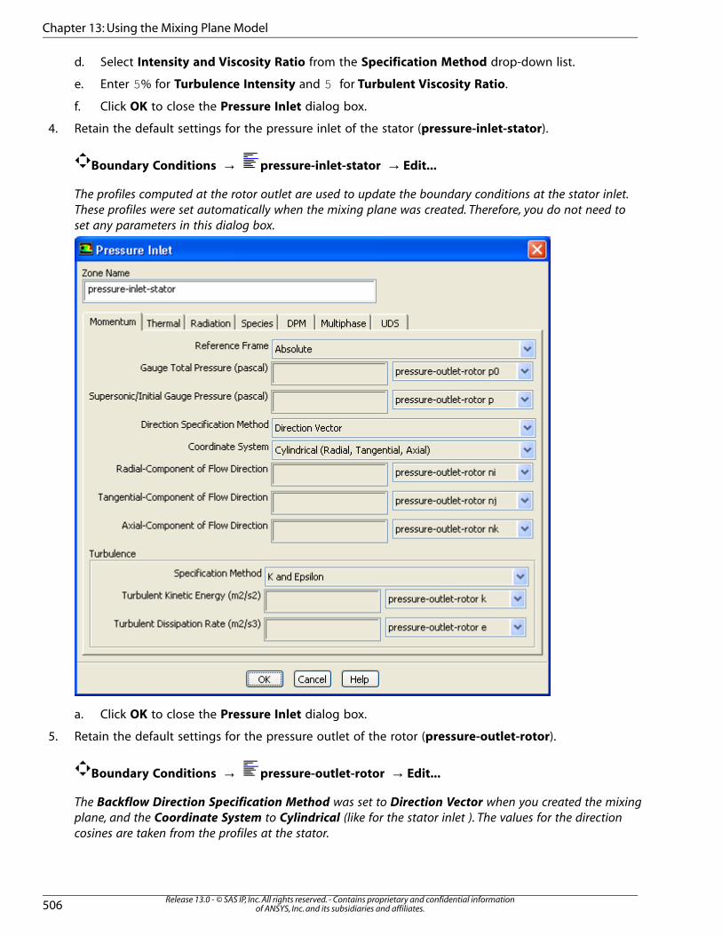
4. Retain the default settings for the pressure inlet of the stator (pressure-inlet-stator).

Boundary Conditions → pressure-inlet-stator → Edit...

The profiles computed at the rotor outlet are used to update the boundary conditions at the stator inlet.

These profiles were set automatically when the mixing plane was created. Therefore, you do not need to

set any parameters in this dialog box.

a. Click OK to close the Pressure Inlet dialog box.

5. Retain the default settings for the pressure outlet of the rotor (pressure-outlet-rotor).

Boundary Conditions → pressure-outlet-rotor → Edit...

The Backflow Direction Specification Method was set to Direction Vector when you created the mixing

plane, and the Coordinate System to Cylindrical (like for the stator inlet ). The values for the direction

cosines are taken from the profiles at the stator.



a. Click OK to close the Pressure Outlet dialog box.

6. Set the conditions for the pressure outlet of the stator (pressure-outlet-stator).

Boundary Conditions → pressure-outlet-stator → Edit...




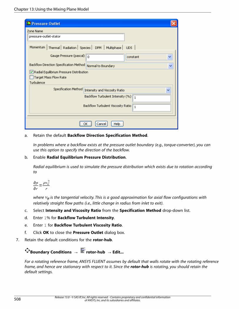
a. Retain the default Backflow Direction Specification Method.

In problems where a backflow exists at the pressure outlet boundary (e.g., torque-converter), you can

use this option to specify the direction of the backflow.

b. Enable Radial Equilibrium Pressure Distribution.

Radial equilibrium is used to simulate the pressure distribution which exists due to rotation according

to

=∂∂

�� where

�� is the tangential velocity. This is a good approximation for axial flow configurations with

relatively straight flow paths (i.e., little change in radius from inlet to exit).

c. Select Intensity and Viscosity Ratio from the Specification Method drop-down list.

d. Enter 1% for Backflow Turbulent Intensity.

e. Enter 1 for Backflow Turbulent Viscosity Ratio.

f. Click OK to close the Pressure Outlet dialog box.

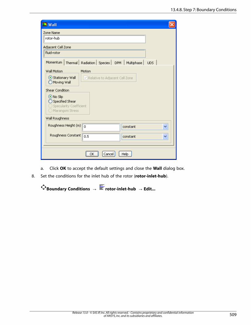
7. Retain the default conditions for the rotor-hub.

Boundary Conditions → rotor-hub → Edit...

For a rotating reference frame, ANSYS FLUENT assumes by default that walls rotate with the rotating reference

frame, and hence are stationary with respect to it. Since the rotor-hub is rotating, you should retain the

default settings.



a. Click OK to accept the default settings and close the Wall dialog box.

8. Set the conditions for the inlet hub of the rotor (rotor-inlet-hub).

Boundary Conditions → rotor-inlet-hub → Edit...




a. Select Moving Wall in the Wall Motion list.

The Wall dialog box will expand to show the wall motion inputs.

b. Select Absolute and Rotational in the Motion group box.

c. Enter -1 for Z in the Rotation-Axis Direction group box.

d. Click OK to close the Wall dialog box.

These conditions set the rotor-inlet-hub to be a stationary wall in the absolute frame.

9. Set the conditions for the shroud of the rotor inlet (rotor-inlet-shroud).

Boundary Conditions → rotor-inlet-shroud → Edit...





c. Enter -1 for Z in the Rotation-Axis Direction group box.


These conditions will set the rotor-inlet-shroud to be a stationary wall in the absolute frame.

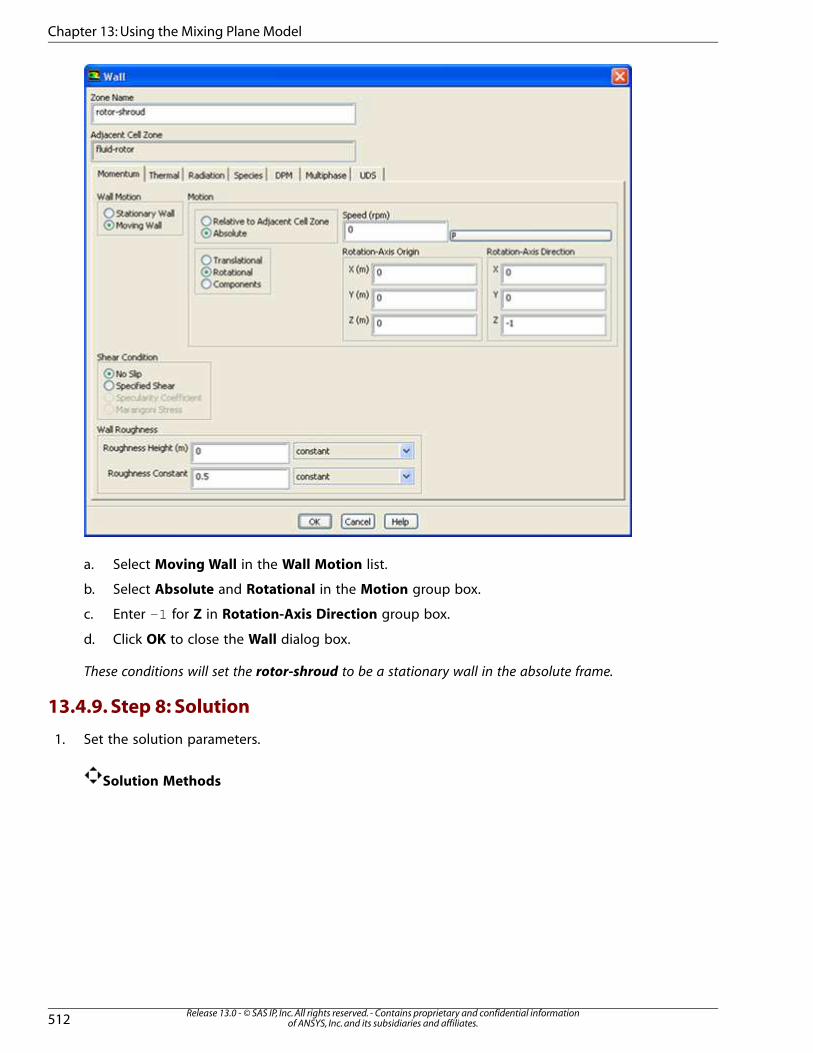
10. Set the conditions for the rotor shroud (rotor-shroud).

Boundary Conditions → rotor-shroud → Edit...






c. Enter -1 for Z in Rotation-Axis Direction group box.


These conditions will set the rotor-shroud to be a stationary wall in the absolute frame.


1. Set the solution parameters.

Solution Methods



a. Select Coupled from Scheme drop-down list in the Pressure-Velocity Coupling group box.

b. Select Second Order Upwind from the Momentum drop-down list in the Spatial Discretizationgroup box.

c. Select Power Law from the Turbulent Kinetic Energy and Turbulent Dissipation Rate drop-

down lists.

d. Enable Pseudo Transient.

2. Set the solution controls.

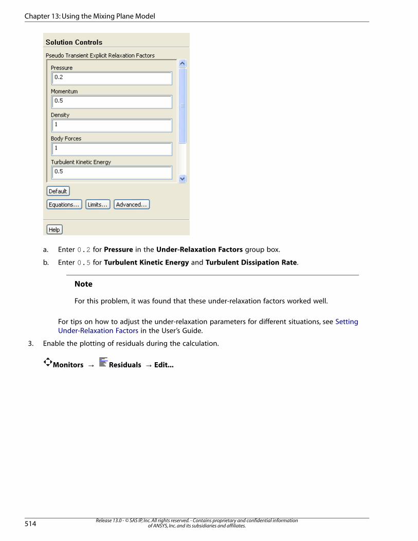
Solution Controls




a. Enter 0.2 for Pressure in the Under-Relaxation Factors group box.

b. Enter 0.5 for Turbulent Kinetic Energy and Turbulent Dissipation Rate.

Note

For this problem, it was found that these under-relaxation factors worked well.

For tips on how to adjust the under-relaxation parameters for different situations, see Setting

Under-Relaxation Factors in the User’s Guide.

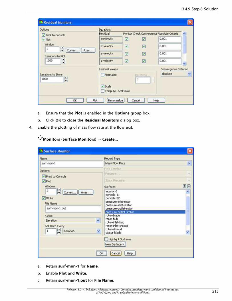
3. Enable the plotting of residuals during the calculation.

Monitors → Residuals → Edit...



a. Ensure that the Plot is enabled in the Options group box.

b. Click OK to close the Residual Monitors dialog box.

4. Enable the plotting of mass flow rate at the flow exit.

Monitors (Surface Monitors) → Create...

a. Retain surf-mon-1 for Name.

b. Enable Plot and Write.

c. Retain surf-mon-1.out for File Name.




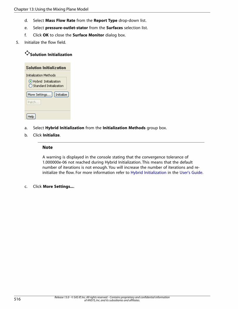
d. Select Mass Flow Rate from the Report Type drop-down list.

e. Select pressure-outlet-stator from the Surfaces selection list.

f. Click OK to close the Surface Monitor dialog box.

5. Initialize the flow field.

Solution Initialization

a. Select Hybrid Initialization from the Initialization Methods group box.

b. Click Initialize.

Note

A warning is displayed in the console stating that the convergence tolerance of

1.000000e-06 not reached during Hybrid Initialization. This means that the default

number of iterations is not enough. You will increase the number of iterations and re-

initialize the flow. For more information refer to Hybrid Initialization in the User's Guide.

c. Click More Settings....



i. Increase the Number of Iterations to 15 .

ii. Click OK and close the Hybrid Initialization dialog box.

d. Click Initialize once more.

Note

Click OK in the Question dialog box, where it asks to discard the current data. The console

displays that hybrid initialization is done.

Note

For flows in complex topologies, hybrid initialization will provide better initial velocity and

pressure fields than standard initialization. This in general will help in improving the conver-

gence behavior of the solver.

6. Save the case file (fanstage.cas.gz ).

File → Write → Case...

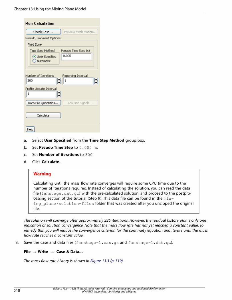
7. Start the calculation by requesting 200 iterations.

Run Calculation




a. Select User Specified from the Time Step Method group box.

b. Set Pseudo Time Step to 0.005 s .

c. Set Number of iterations to 300 .

d. Click Calculate.

Warning

Calculating until the mass flow rate converges will require some CPU time due to the

number of iterations required. Instead of calculating the solution, you can read the data

file (fanstage.dat.gz ) with the pre-calculated solution, and proceed to the postpro-

cessing section of the tutorial (Step 9). This data file can be found in the mix-ing_plane/solution-files folder that was created after you unzipped the original

file.

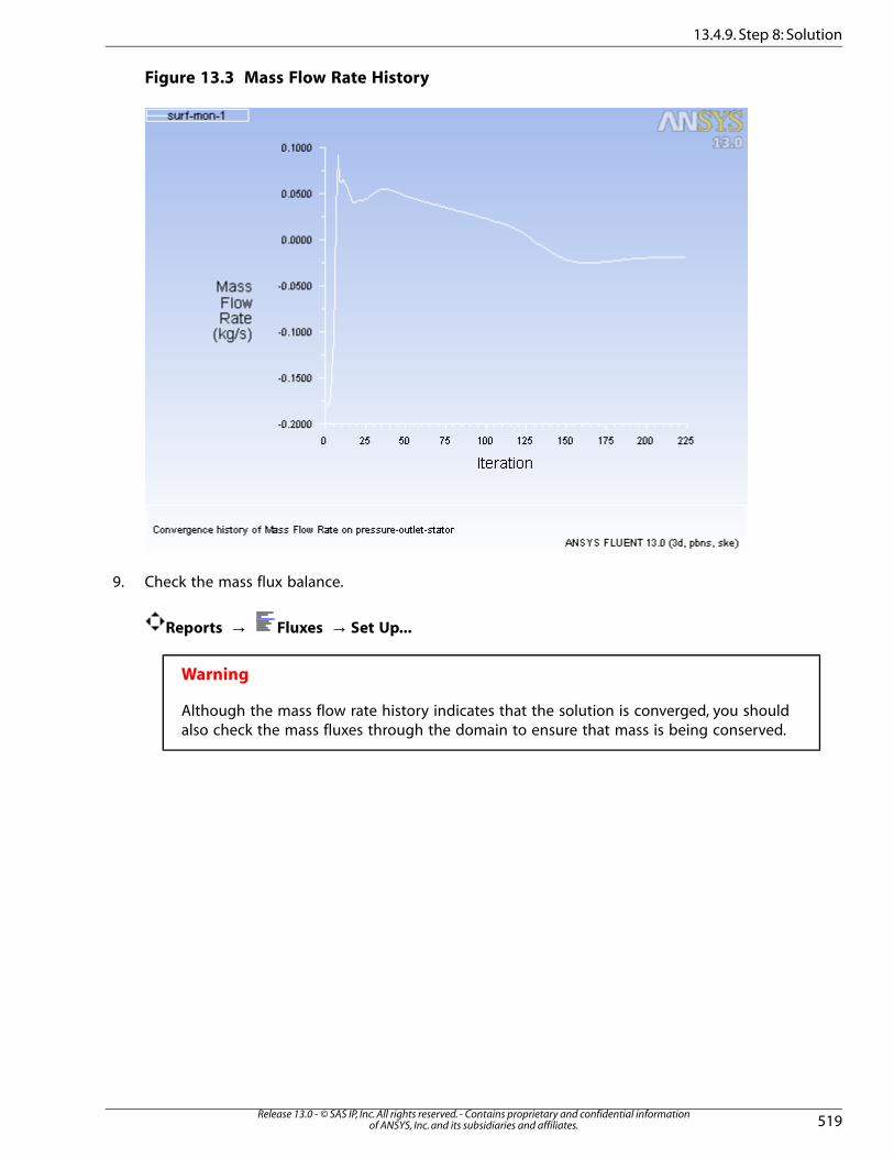
The solution will converge after approximately 225 iterations. However, the residual history plot is only one

indication of solution convergence. Note that the mass flow rate has not yet reached a constant value. To

remedy this, you will reduce the convergence criterion for the continuity equation and iterate until the mass

flow rate reaches a constant value.

8. Save the case and data files (fanstage-1.cas.gz and fanstage-1.dat.gz ).

File → Write → Case & Data...

The mass flow rate history is shown in Figure 13.3 (p. 519).



Figure 13.3 Mass Flow Rate History

9. Check the mass flux balance.

Reports → Fluxes → Set Up...

Warning

Although the mass flow rate history indicates that the solution is converged, you should

also check the mass fluxes through the domain to ensure that mass is being conserved.




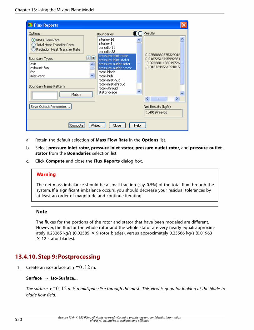
a. Retain the default selection of Mass Flow Rate in the Options list.

b. Select pressure-inlet-rotor, pressure-inlet-stator, pressure-outlet-rotor, and pressure-outlet-stator from the Boundaries selection list.

c. Click Compute and close the Flux Reports dialog box.

Warning

The net mass imbalance should be a small fraction (say, 0.5%) of the total flux through the

system. If a significant imbalance occurs, you should decrease your residual tolerances by

at least an order of magnitude and continue iterating.

Note

The fluxes for the portions of the rotor and stator that have been modeled are different.

However, the flux for the whole rotor and the whole stator are very nearly equal: approxim-

ately 0.23265 kg/s (0.02585 × 9 rotor blades), versus approximately 0.23566 kg/s (0.01963

× 12 stator blades).


1. Create an isosurface at =� m.

Surface → Iso-Surface...

The surface =� m is a midspan slice through the mesh. This view is good for looking at the blade-to-

blade flow field.



a. Select Mesh... and Y-Coordinate from the Surface of Constant drop-down lists.

b. Click Compute to update the minimum and maximum values.

c. Enter 0.12 for Iso-Values.

d. Enter y=0.12 for New Surface Name.

e. Click Create to create the isosurface.

2. Create an isosurface at = −� m.

Surface → Iso-Surface...

The surface = −� m is an axial plane downstream of the stator. This will be used to plot circumferentially-

averaged profiles.

a. Select Mesh... and Z-Coordinate from the Surface of Constant drop-down lists.

b. Click Compute to update the minimum and maximum values.

c. Enter -0.1 for Iso-Values.

d. Enter z=-0.1 for New Surface Name.

Note

The default name that ANSYS FLUENT displays in the New Surface Name field (i.e., z-coordinate-17) indicates that this is surface number 17. This fact will be used later in

the tutorial when you plot circumferential averages.

e. Click Create to create the isosurface.

f. Close the Iso-Surface dialog box.

3. Display velocity vectors on the midspan surface =� (Figure 13.4 (p. 523)).

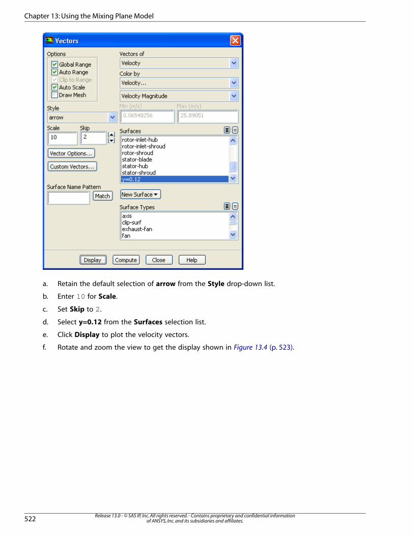
Graphics and Animations → Vectors → Set Up...




a. Retain the default selection of arrow from the Style drop-down list.

b. Enter 10 for Scale.

c. Set Skip to 2.

d. Select y=0.12 from the Surfaces selection list.

e. Click Display to plot the velocity vectors.

f. Rotate and zoom the view to get the display shown in Figure 13.4 (p. 523).



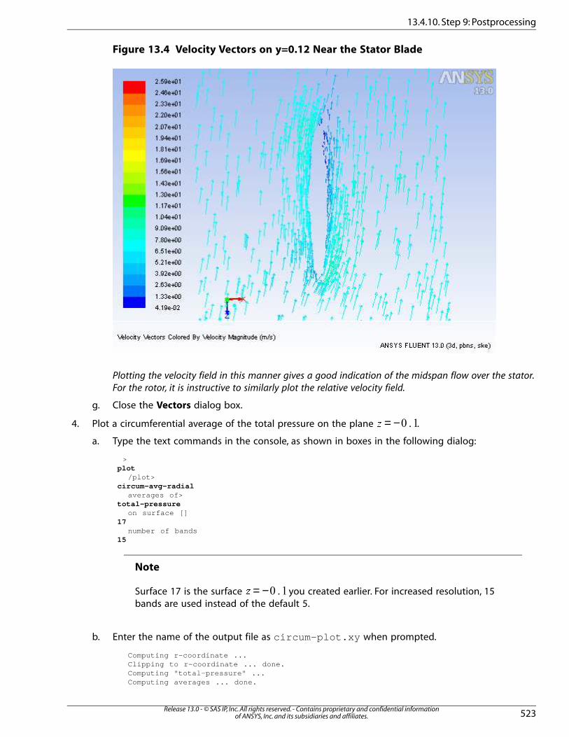
Figure 13.4 Velocity Vectors on y=0.12 Near the Stator Blade

Plotting the velocity field in this manner gives a good indication of the midspan flow over the stator.

For the rotor, it is instructive to similarly plot the relative velocity field.

g. Close the Vectors dialog box.

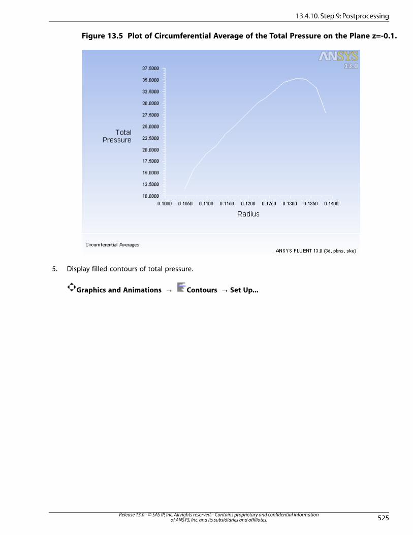
4. Plot a circumferential average of the total pressure on the plane = −�.

a. Type the text commands in the console, as shown in boxes in the following dialog:

>plot /plot> circum-avg-radial averages of> total-pressure on surface [] 17 number of bands 15

Note

Surface 17 is the surface = −� you created earlier. For increased resolution, 15

bands are used instead of the default 5.

b. Enter the name of the output file as circum-plot.xy when prompted.

Computing r-coordinate ... Clipping to r-coordinate ... done. Computing "total-pressure" ... Computing averages ... done.




Creating radial-bands surface (32 31 30 29 28 27 26 25 24 23 22 21 20 19 18). filename [""] "circum-plot.xy" order points? [no]

c. Retain the default of no when asked to order points .

d. Display the circumferential average.

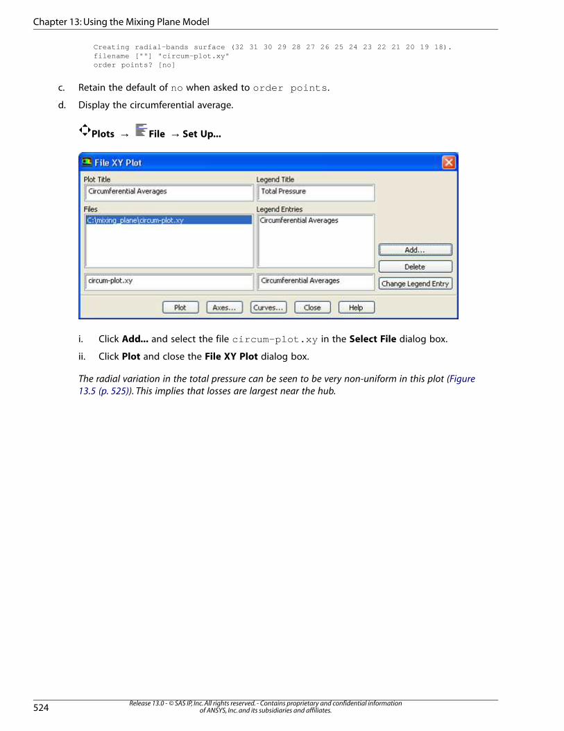
Plots → File → Set Up...

i. Click Add... and select the file circum-plot.xy in the Select File dialog box.

ii. Click Plot and close the File XY Plot dialog box.

The radial variation in the total pressure can be seen to be very non-uniform in this plot (Figure

13.5 (p. 525)). This implies that losses are largest near the hub.



Figure 13.5 Plot of Circumferential Average of the Total Pressure on the Plane z=-0.1.

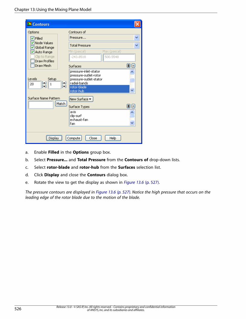
5. Display filled contours of total pressure.

Graphics and Animations → Contours → Set Up...




a. Enable Filled in the Options group box.

b. Select Pressure... and Total Pressure from the Contours of drop-down lists.

c. Select rotor-blade and rotor-hub from the Surfaces selection list.

d. Click Display and close the Contours dialog box.

e. Rotate the view to get the display as shown in Figure 13.6 (p. 527).

The pressure contours are displayed in Figure 13.6 (p. 527). Notice the high pressure that occurs on the

leading edge of the rotor blade due to the motion of the blade.



Figure 13.6 Contours of Total Pressure for the Rotor Blade and Hub

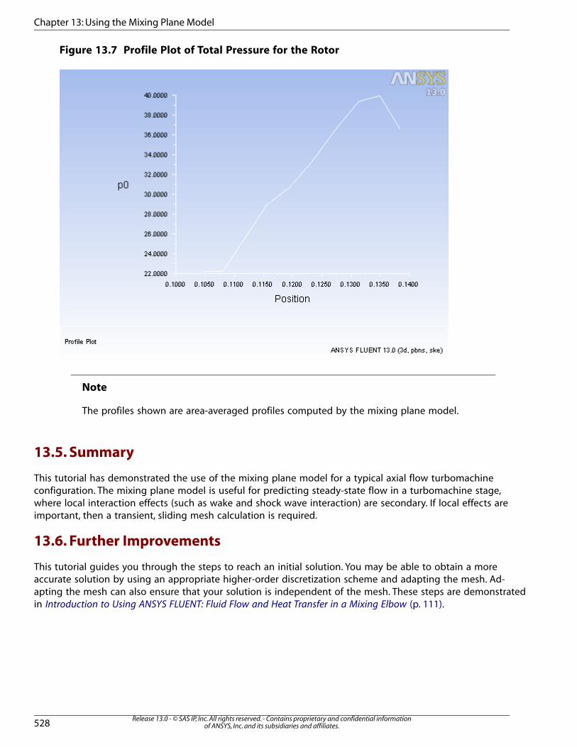
6. Display the total pressure profiles at the outlet of the rotor.

Plots → Profile Data → Set Up...

a. Retain pressure-outlet-rotor from the Profile selection list.

b. Ensure that p0 is selected from the Y Axis Function selection list.

c. Click Plot and close the Plot Profile Data dialog box.




Figure 13.7 Profile Plot of Total Pressure for the Rotor

Note

The profiles shown are area-averaged profiles computed by the mixing plane model.

13.5. Summary

This tutorial has demonstrated the use of the mixing plane model for a typical axial flow turbomachine

configuration. The mixing plane model is useful for predicting steady-state flow in a turbomachine stage,

where local interaction effects (such as wake and shock wave interaction) are secondary. If local effects are

important, then a transient, sliding mesh calculation is required.

13.6. Further Improvements

This tutorial guides you through the steps to reach an initial solution. You may be able to obtain a more

accurate solution by using an appropriate higher-order discretization scheme and adapting the mesh. Ad-

apting the mesh can also ensure that your solution is independent of the mesh. These steps are demonstrated

in Introduction to Using ANSYS FLUENT: Fluid Flow and Heat Transfer in a Mixing Elbow (p. 111).



Date post:	06-Jul-2018
Category:	Documents
Upload:	phungthuan
View:	236 times
Download:	0 times

Chapter 13: Using the Mixing Plane Model · Fluid Flow and Heat Transfer in a Mixing Elbow ......

Documents