65
Chapter 14: Numerical Methods
| Date post: | 26-Dec-2015 |
| Category: |
Documents |
| Upload: | carol-ryan |
| View: | 252 times |
| Download: | 2 times |

Chapter 14:Numerical Methods
• In this chapter, you will learn about:– Root finding– The bisection method– Refinements to the bisection method– The secant method– Numerical integration– The trapezoidal rule– Simpson’s rule– Common programming errors
Objectives
2C++ for Engineers and Scientists, Fourth Edition
• Root finding is useful in solving engineering problems
• Vital elements in numerical analysis are: – Appreciating what can or can’t be solved – Clearly understanding the accuracy of answers found
Introduction to Root Finding
3C++ for Engineers and Scientists, Fourth Edition

• Examples of the types of functions encountered in root-solving problems:
Introduction to Root Finding (continued)
4C++ for Engineers and Scientists, Fourth Edition
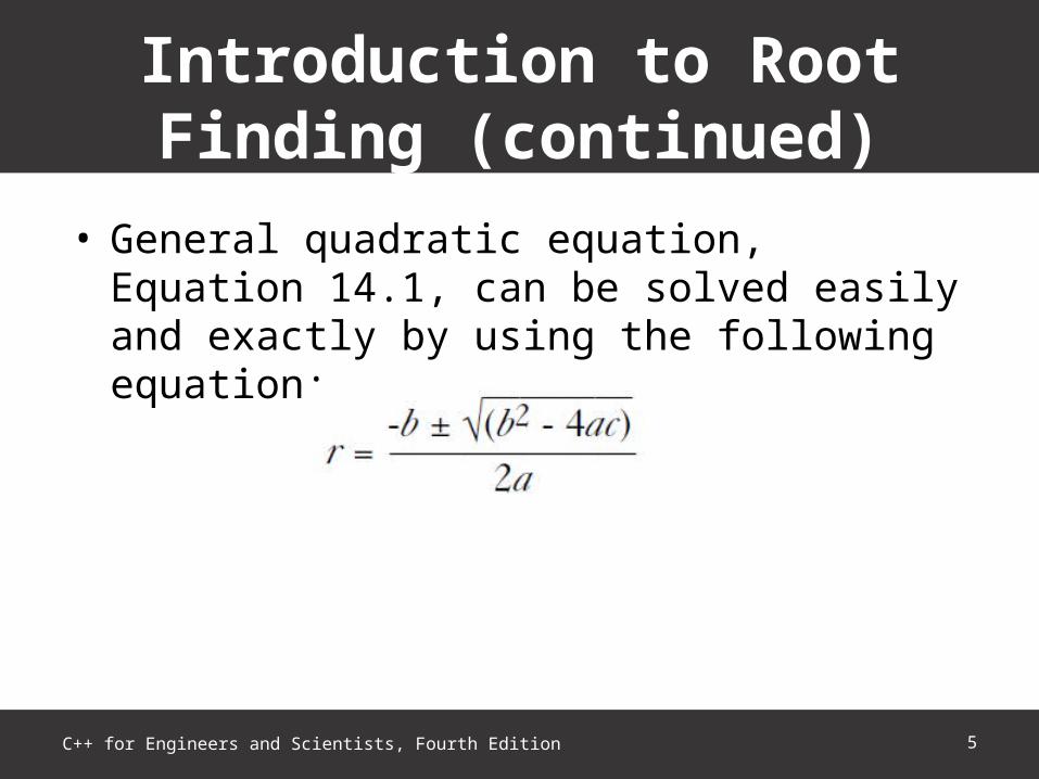
• General quadratic equation, Equation 14.1, can be solved easily and exactly by using the following equation:
Introduction to Root Finding (continued)
5C++ for Engineers and Scientists, Fourth Edition
• Equation 14.2 can be solved for x exactly by factoring the polynomial
• Equations 14.4 and 14.5 are transcendental equations
• Transcendental equations– Represent a different class of functions– Typically involve trigonometric, exponential, or
logarithmic functions– Cannot be reduced to any polynomial equation in x
Introduction to Root Finding (continued)
6C++ for Engineers and Scientists, Fourth Edition
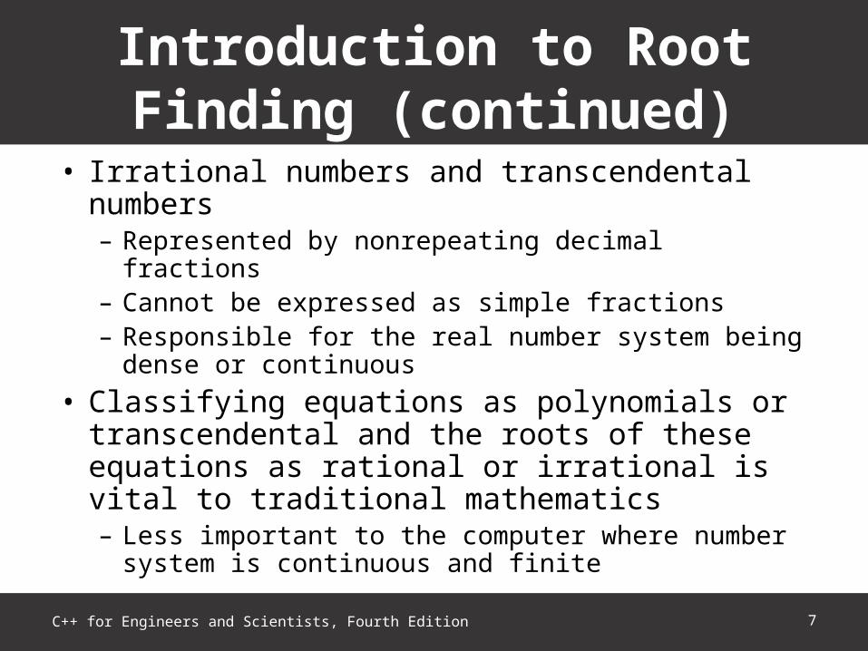
• Irrational numbers and transcendental numbers– Represented by nonrepeating decimal fractions – Cannot be expressed as simple fractions– Responsible for the real number system being dense or
continuous• Classifying equations as polynomials or
transcendental and the roots of these equations as rational or irrational is vital to traditional mathematics– Less important to the computer where number system is
continuous and finite
Introduction to Root Finding (continued)
7C++ for Engineers and Scientists, Fourth Edition

• When finding roots of equations, the distinction between polynomials and transcendental equations is unnecessary
• Many theorems learned for roots and polynomials don’t apply to transcendental equations– Both Equations 14.4 and 14.5 have infinite number of real
roots
Introduction to Root Finding (continued)
8C++ for Engineers and Scientists, Fourth Edition
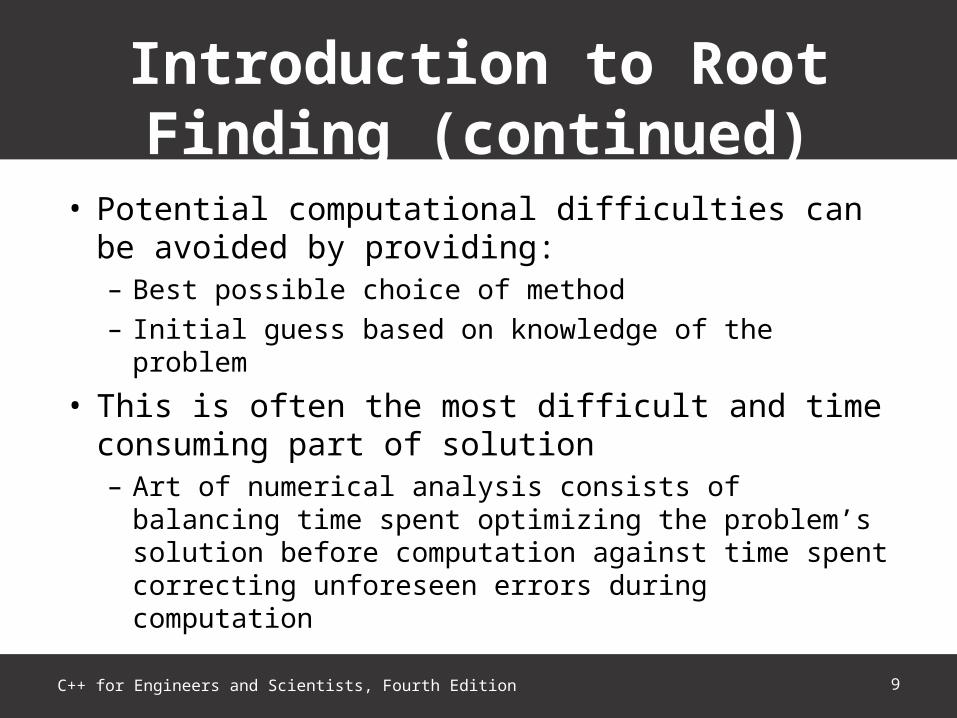
• Potential computational difficulties can be avoided by providing:– Best possible choice of method– Initial guess based on knowledge of the problem
• This is often the most difficult and time consuming part of solution– Art of numerical analysis consists of balancing time spent
optimizing the problem’s solution before computation against time spent correcting unforeseen errors during computation
Introduction to Root Finding (continued)
9C++ for Engineers and Scientists, Fourth Edition

• Sketch function before attempting root solving– Use graphing routines or– Generate table of function values and graph by hand
• Graphs are useful to programmers in: – Estimating first guess for root – Anticipating potential difficulties
Introduction to Root Finding (continued)
10C++ for Engineers and Scientists, Fourth Edition
Introduction to Root Finding (continued)
11C++ for Engineers and Scientists, Fourth Edition
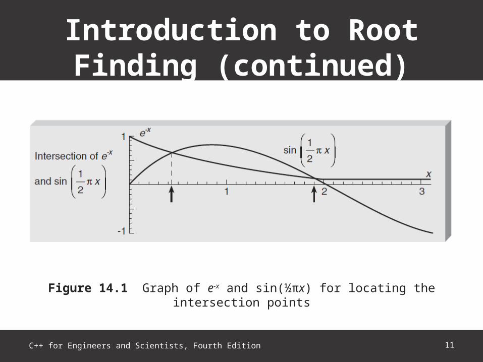
Figure 14.1 Graph of e-x and sin(½πx) for locating the intersection points
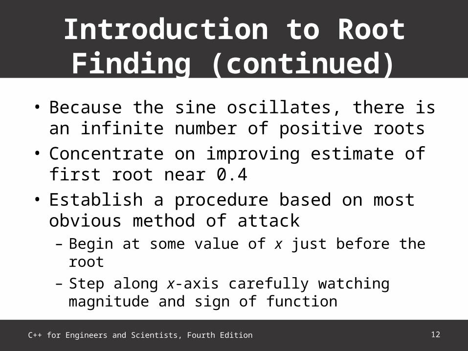
• Because the sine oscillates, there is an infinite number of positive roots
• Concentrate on improving estimate of first root near 0.4
• Establish a procedure based on most obvious method of attack– Begin at some value of x just before the root– Step along x-axis carefully watching magnitude and sign
of function
Introduction to Root Finding (continued)
12C++ for Engineers and Scientists, Fourth Edition

• Notice that function changed sign between 0.4 and 0.5– Indicates root between these two x values
Introduction to Root Finding (continued)
13C++ for Engineers and Scientists, Fourth Edition

• For next approximation use midpoint value, x = 0.45
• Function is again negative at 0.45 indicating root between 0.4 and 0.45
• Next approximation is midpoint, 0.425
Introduction to Root Finding (continued)
14C++ for Engineers and Scientists, Fourth Edition

• In this way, proceed systematically to a computation of the root to any degree of accuracy
• Key element in this procedure is monitoring the sign of function
• When sign changes, specific action is taken to refine estimate of root
Introduction to Root Finding (continued)
15C++ for Engineers and Scientists, Fourth Edition
• Root-solving procedure previously explained is suitable for hand calculations
• A slight modification makes it more systematic and easier to adapt to computer coding
• Modified computational technique is known as the bisection method– Suppose you already know there’s a root between x = a and x = b
• Function changes sign in this interval– Assume
• Only one root between x = a and x = b• Function is continuous in this interval
The Bisection Method
16C++ for Engineers and Scientists, Fourth Edition
The Bisection Method (continued)
17C++ for Engineers and Scientists, Fourth Edition
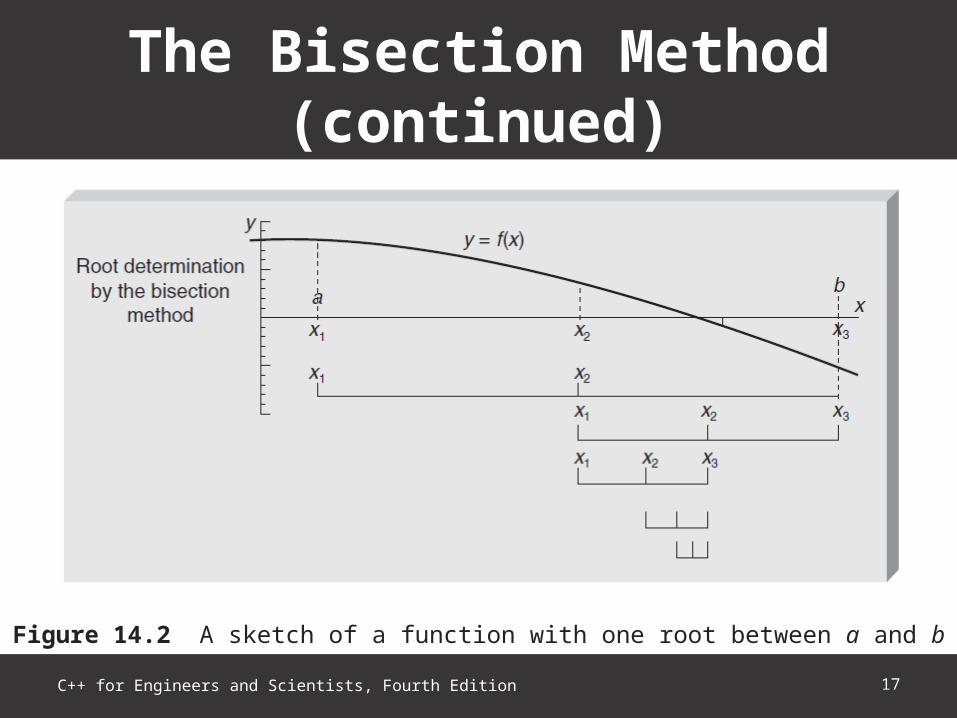
Figure 14.2 A sketch of a function with one root between a and b
• After determining a second time whether the left or right half contains the root, interval is again replaced by the left or right half-interval
• Continue process until narrow in on the root at previously assigned accuracy
• Each step halves interval– After n intervals, interval’s size containing root is
• (b – a)/2n
The Bisection Method (continued)
18C++ for Engineers and Scientists, Fourth Edition
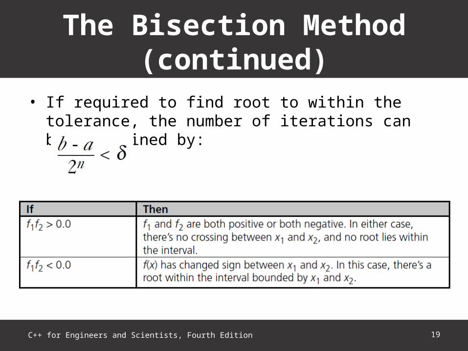
• If required to find root to within the tolerance, the number of iterations can be determined by:
The Bisection Method (continued)
19C++ for Engineers and Scientists, Fourth Edition

• Program 14.1 computes roots of equations• Note the following features:
– In each iteration after the first one, there is only one function evaluation
– Program contains several checks for potential problems along with diagnostic messages along with diagnostic messages
– Criterion for success is based on interval’s size
The Bisection Method (continued)
20C++ for Engineers and Scientists, Fourth Edition
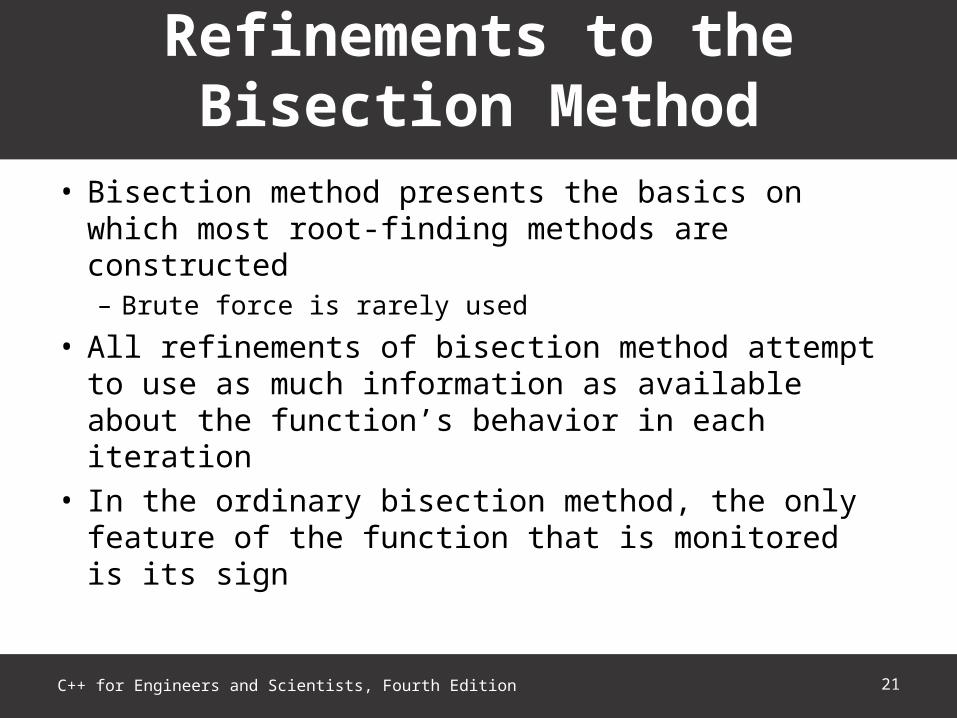
• Bisection method presents the basics on which most root-finding methods are constructed– Brute force is rarely used
• All refinements of bisection method attempt to use as much information as available about the function’s behavior in each iteration
• In the ordinary bisection method, the only feature of the function that is monitored is its sign
Refinements to the Bisection Method
21C++ for Engineers and Scientists, Fourth Edition
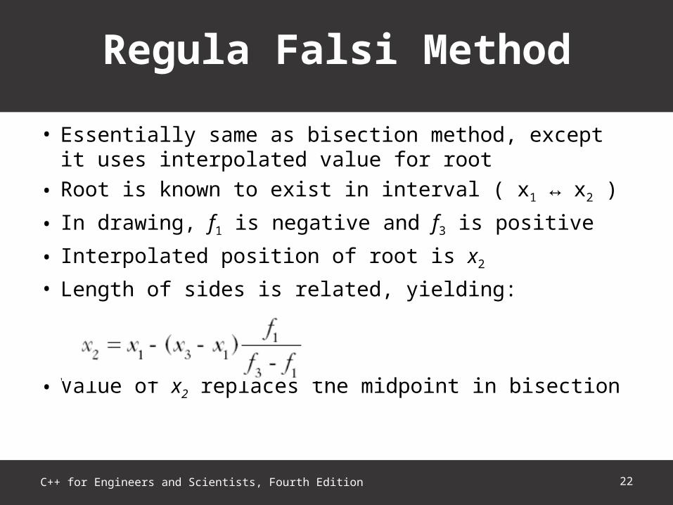
• Essentially same as bisection method, except it uses interpolated value for root
• Root is known to exist in interval ( x1 ↔ x2 )
• In drawing, f1 is negative and f3 is positive
• Interpolated position of root is x2
• Length of sides is related, yielding:
• Value of x2 replaces the midpoint in bisection
Regula Falsi Method
22C++ for Engineers and Scientists, Fourth Edition

23C++ for Engineers and Scientists, Fourth Edition
Figure 14.3 Estimating the root by interpolation
Regula Falsi Method (continued)
24C++ for Engineers and Scientists, Fourth Edition
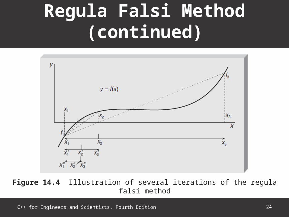
Figure 14.4 Illustration of several iterations of the regula falsi method
Regula Falsi Method (continued)

• Perhaps the procedure can be made to collapse from both directions from both directions
• The idea is as follows:
Modified Regula Falsi Method
25C++ for Engineers and Scientists, Fourth Edition

26C++ for Engineers and Scientists, Fourth Edition
Figure 14.5 Illustration of the modified regula falsi method
Modified Regula Falsi Method (continued)

• Using this algorithm, slope of line is reduced artificially
• If root is in left of original interval, it: – Eventually turns up in the right segment of a later interval– Subsequently alternates between left and right
Modified Regula Falsi Method (continued)
27C++ for Engineers and Scientists, Fourth Edition
Modified Regula Falsi Method (continued)
28C++ for Engineers and Scientists, Fourth Edition
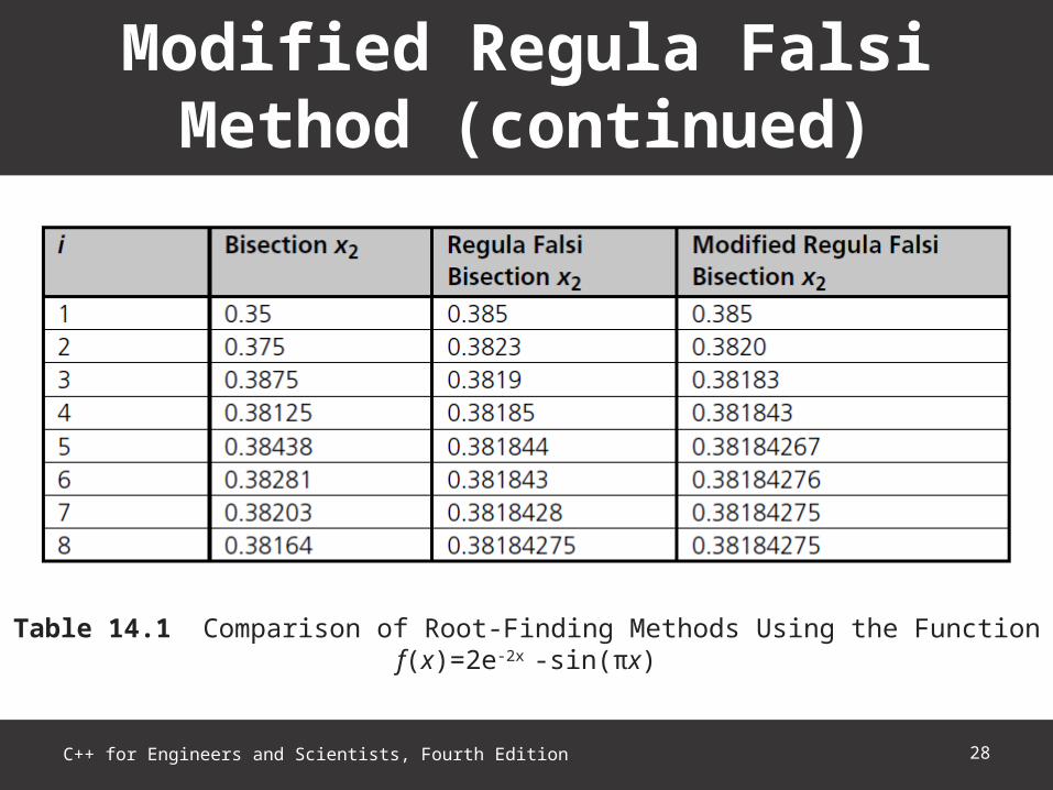
Table 14.1 Comparison of Root-Finding Methods Using the Function f(x)=2e-2x -sin(πx)

• Relaxation factor: Number used to alter the results of one iteration before inserting them into the next
• Trial and error shows that a less drastic increase in the slope results in improved convergence
• Using a convergence factor of 0.9 should be adequate for most problems
Modified Regula Falsi Method (continued)
29C++ for Engineers and Scientists, Fourth Edition
• Bisection– Success based on size of interval– Slow convergence– Predictable number of iterations– Interval halved in each iteration– Guaranteed to bracket a root
Summary of the Bisection Methods
30C++ for Engineers and Scientists, Fourth Edition

• Regula falsi– Success based on size of function– Faster convergence– Unpredictable number of iterations– Interval containing the root is not small
Summary of the Bisection Methods (continued)
31C++ for Engineers and Scientists, Fourth Edition

• Modified regula falsi– Success based on size of interval– Faster convergence– Unpredictable number of iterations– Of three methods, most efficient for common problems
Summary of the Bisection Methods (continued)
32C++ for Engineers and Scientists, Fourth Edition

• Identical to regula falsi method except sign of f(x) doesn’t need to be checked at each iteration
The Secant Method
33C++ for Engineers and Scientists, Fourth Edition
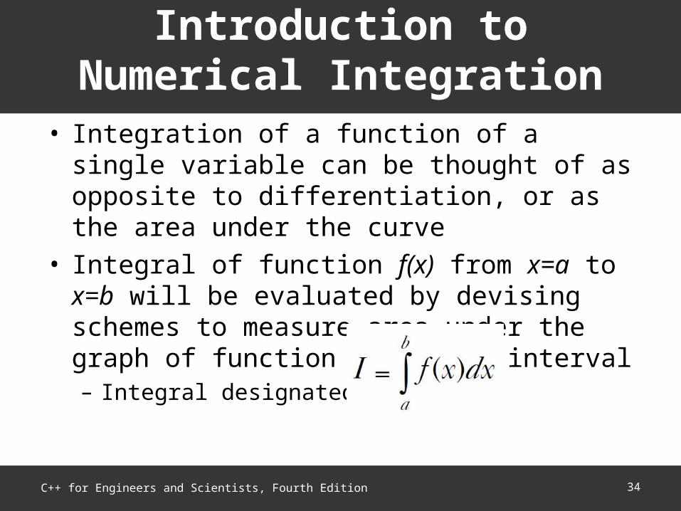
• Integration of a function of a single variable can be thought of as opposite to differentiation, or as the area under the curve
• Integral of function f(x) from x=a to x=b will be evaluated by devising schemes to measure area under the graph of function over this interval– Integral designated as:
Introduction to Numerical Integration
34C++ for Engineers and Scientists, Fourth Edition

35C++ for Engineers and Scientists, Fourth Edition
Figure 14.7 An integral as an area under a curve
Introduction to Numerical Integration (continued)

• Numerical integration is a stable process– Consists of expressing the area as the sum of areas of
smaller segments– Fairly safe from division by zero or round-off errors
caused by subtracting numbers of approximately the same magnitude
• Many integrals in engineering or science cannot be expressed in any closed form
Introduction to Numerical Integration (continued)
36C++ for Engineers and Scientists, Fourth Edition
• Trapezoidal rule approximation for integral– Replace function over limited range by straight line
segments– Interval x=a to x=b is divided into subintervals of size ∆x– Function replaced by line segments over each subinterval– Area under function is then approximated by area under
line segments
Introduction to Numerical Integration (continued)
37C++ for Engineers and Scientists, Fourth Edition
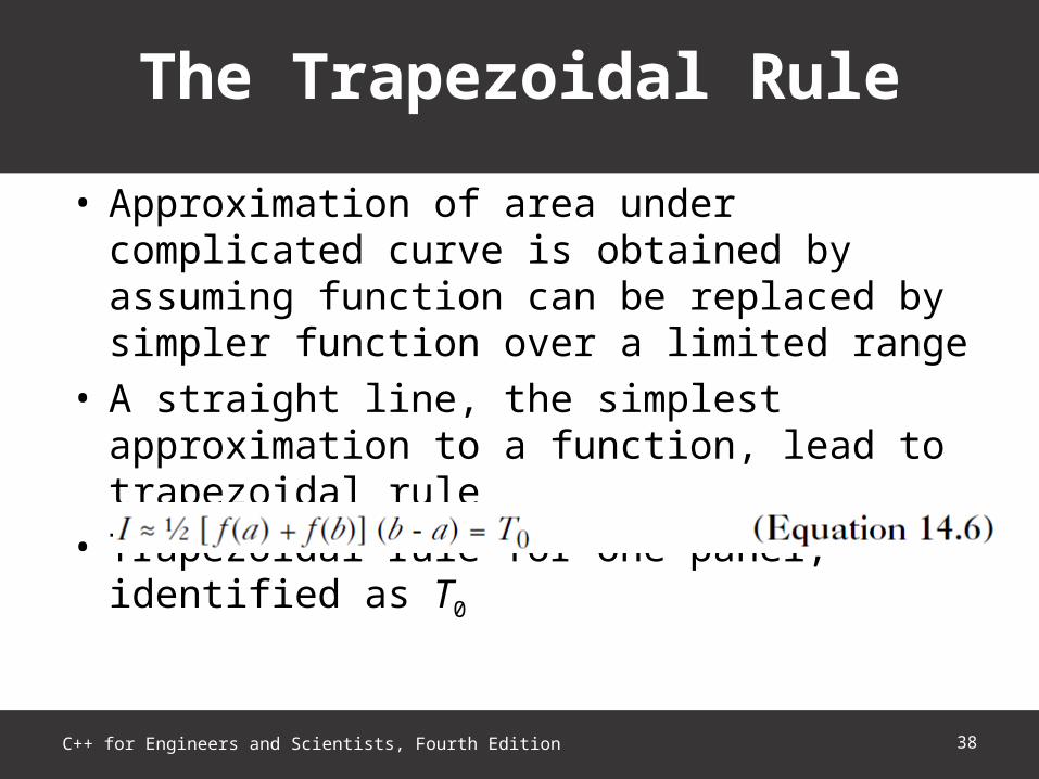
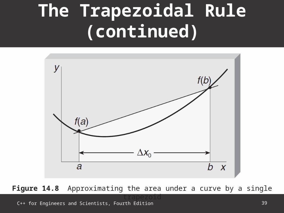
• Approximation of area under complicated curve is obtained by assuming function can be replaced by simpler function over a limited range
• A straight line, the simplest approximation to a function, lead to trapezoidal rule
• Trapezoidal rule for one panel, identified as T0
The Trapezoidal Rule
38C++ for Engineers and Scientists, Fourth Edition
39C++ for Engineers and Scientists, Fourth Edition
Figure 14.8 Approximating the area under a curve by a single trapezoid
The Trapezoidal Rule (continued)

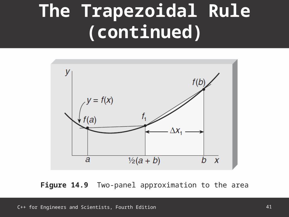
• Improve accuracy of approximation under curve by dividing interval in half– Function is approximated by straight-line segments over
each half
• Area in example is approximated by area of two trapezoids
The Trapezoidal Rule (continued)
40C++ for Engineers and Scientists, Fourth Edition
41C++ for Engineers and Scientists, Fourth Edition
Figure 14.9 Two-panel approximation to the area
The Trapezoidal Rule (continued)
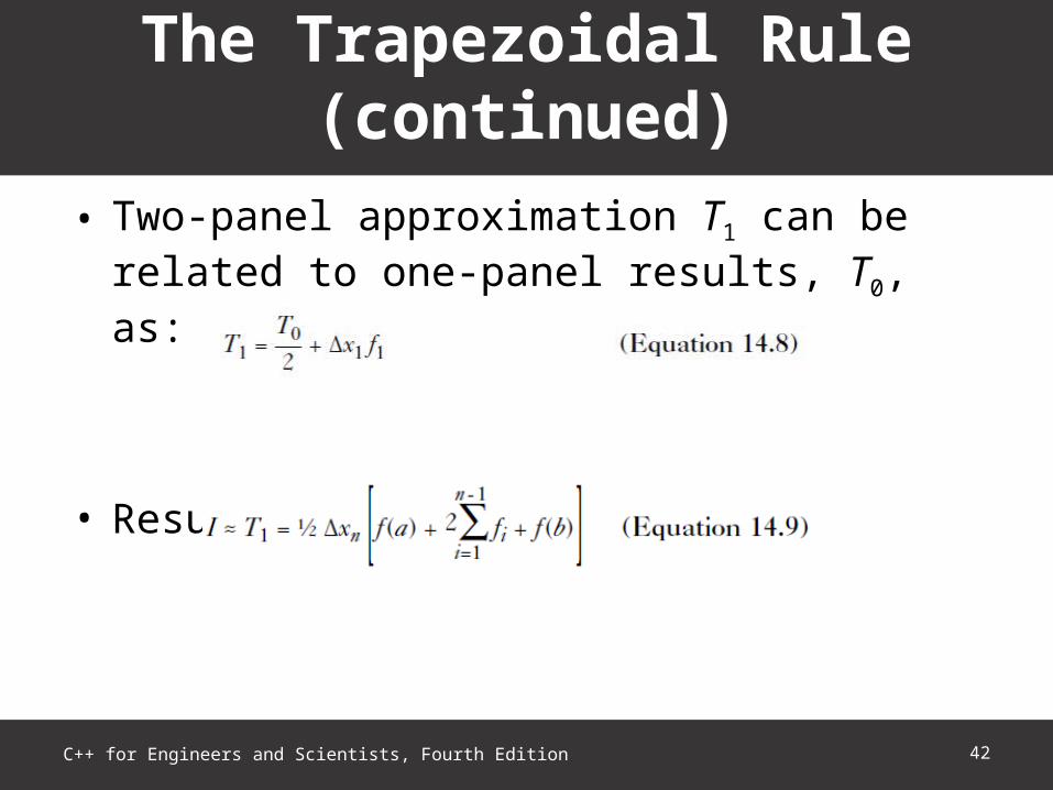
• Two-panel approximation T1 can be related to one-panel results, T0, as:
• Result for n panels is:
The Trapezoidal Rule (continued)
42C++ for Engineers and Scientists, Fourth Edition
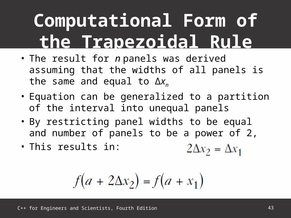
• The result for n panels was derived assuming that the widths of all panels is the same and equal to ∆xn
• Equation can be generalized to a partition of the interval into unequal panels
• By restricting panel widths to be equal and number of panels to be a power of 2,
• This results in:
Computational Form of the Trapezoidal Rule
43C++ for Engineers and Scientists, Fourth Edition

44C++ for Engineers and Scientists, Fourth Edition
Figure 14.10 Four-panel trapezoidal approximation, T2
Computational Form of the Trapezoidal Rule (continued)

Computational Form of the Trapezoidal Rule (continued)
45C++ for Engineers and Scientists, Fourth Edition
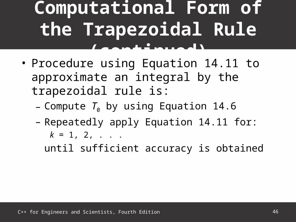
• Procedure using Equation 14.11 to approximate an integral by the trapezoidal rule is:– Compute T0 by using Equation 14.6
– Repeatedly apply Equation 14.11 for: k = 1, 2, . . .
until sufficient accuracy is obtained
Computational Form of the Trapezoidal Rule (continued)
46C++ for Engineers and Scientists, Fourth Edition

• Given the following integral:
• Trapezoidal rule approximation to the integral with a = 1 and b = 2 begins with Equation 14.6 to obtain T0
Example of a Trapezoidal Rule Calculation
47C++ for Engineers and Scientists, Fourth Edition
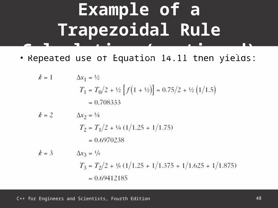
• Repeated use of Equation 14.11 then yields:
Example of a Trapezoidal Rule Calculation (continued)
48C++ for Engineers and Scientists, Fourth Edition
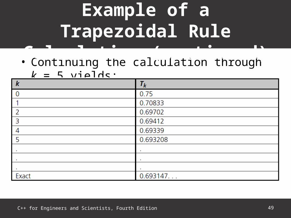
• Continuing the calculation through k = 5 yields:
Example of a Trapezoidal Rule Calculation (continued)
49C++ for Engineers and Scientists, Fourth Edition
• Trapezoidal rule is based on approximating the function by straight-line segments
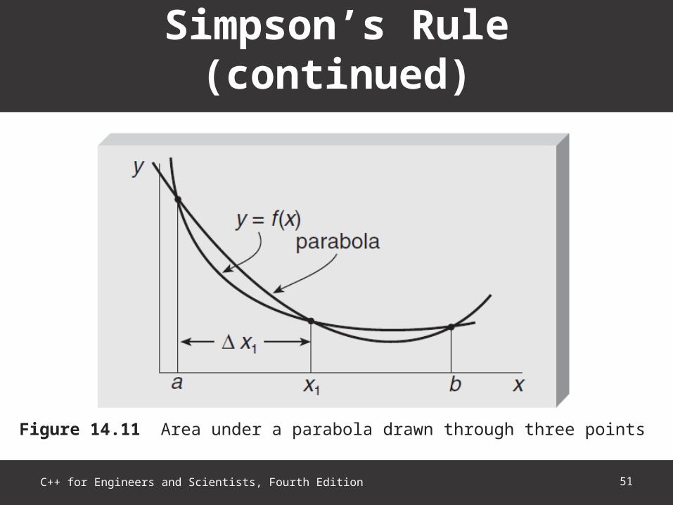
• To improve the accuracy and convergence rate, another approach is approximating the function by parabolic segments– This is known as Simpson’s rule
• Specifying a parabola uniquely requires three points, so the lowest order Simpson’s rule has two panels
Simpson’s Rule
50C++ for Engineers and Scientists, Fourth Edition
51C++ for Engineers and Scientists, Fourth Edition
Figure 14.11 Area under a parabola drawn through three points
Simpson’s Rule (continued)
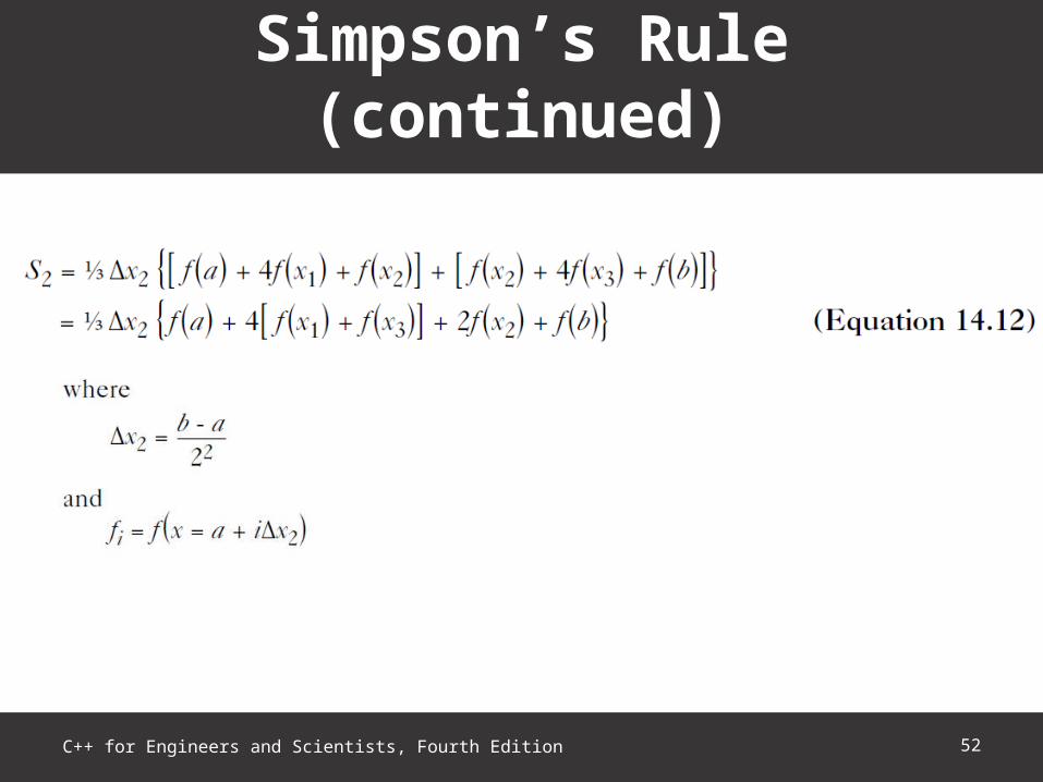
Simpson’s Rule (continued)
52C++ for Engineers and Scientists, Fourth Edition
53C++ for Engineers and Scientists, Fourth Edition
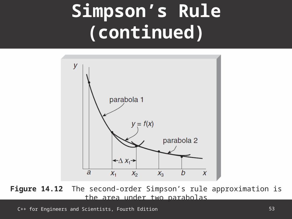
Figure 14.12 The second-order Simpson’s rule approximation is the area under two parabolas
Simpson’s Rule (continued)

• Generalization of Equation 14.12 for n = 2k panels
Simpson’s Rule (continued)
54C++ for Engineers and Scientists, Fourth Edition

• Consider this integral:
• Using Equation 14.13 first for k = 1 yields:
Example of Simpson’s Rule as an Approximation to an Integral
55C++ for Engineers and Scientists, Fourth Edition
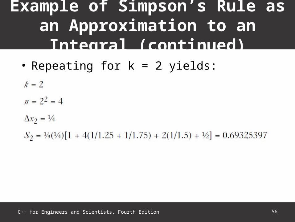
• Repeating for k = 2 yields:
Example of Simpson’s Rule as an Approximation to an Integral (continued)
56C++ for Engineers and Scientists, Fourth Edition

• Continuing the calculation yields:
Example of Simpson’s Rule as an Approximation to an Integral (continued)
57C++ for Engineers and Scientists, Fourth Edition
Figure 14.2 Trapezoidal and Simpson’s rule results for integral

• Two characteristics of this type of computation:– Round-off errors occur when the values of f(x1) and f(x3)
are nearly equal– Prediction of exact number of iterations is not available
• Excessive and possibly infinite iterations must be prevented
• Excessive computation time might be a problem– Occurs if number of iterations exceeds fifty
Common Programming Errors
58C++ for Engineers and Scientists, Fourth Edition

• All root solving methods described in chapter are iterative
• Can be categorized into two classes– Starting from an interval containing a root– Starting from an initial estimate of a root
• Bisection algorithms refine initial interval by:– Repeated evaluation of function at points within interval– Monitoring the sign of the function and determining in
which subinterval the root lies
Summary
59C++ for Engineers and Scientists, Fourth Edition
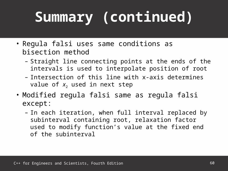
• Regula falsi uses same conditions as bisection method– Straight line connecting points at the ends of the intervals
is used to interpolate position of root– Intersection of this line with x-axis determines value of x2
used in next step
• Modified regula falsi same as regula falsi except:– In each iteration, when full interval replaced by
subinterval containing root, relaxation factor used to modify function’s value at the fixed end of the subinterval
Summary (continued)
60C++ for Engineers and Scientists, Fourth Edition
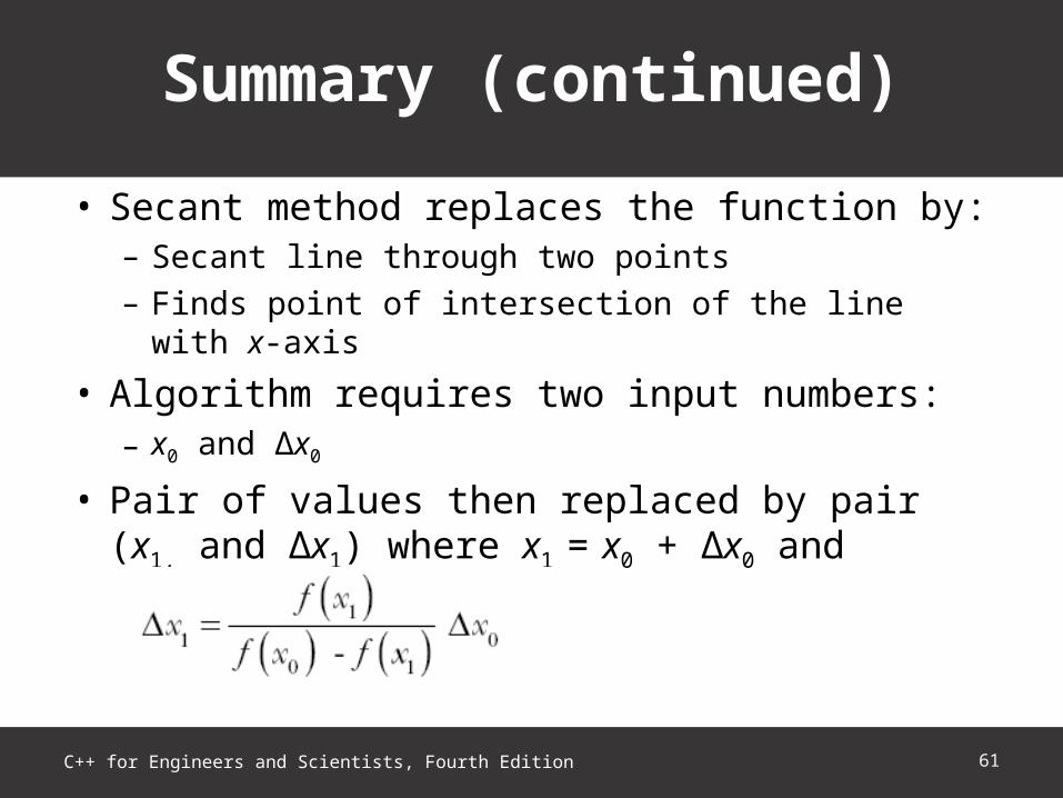
• Secant method replaces the function by:– Secant line through two points– Finds point of intersection of the line with x-axis
• Algorithm requires two input numbers:– x0 and ∆x0
• Pair of values then replaced by pair (x1, and ∆x1) where x1 = x0 + ∆x0 and
Summary (continued)
61C++ for Engineers and Scientists, Fourth Edition
• Secant method processing continues until ∆x is sufficiently small
• Success of a program in finding the root of function usually depends on the quality of information supplied by the user– Accuracy of initial guess or search interval– Method selection match to circumstances of problem
• Execution-time problems are usually traceable to:– Errors in coding– Inadequate user-supplied diagnostics
Chapter Summary (continued)
62C++ for Engineers and Scientists, Fourth Edition
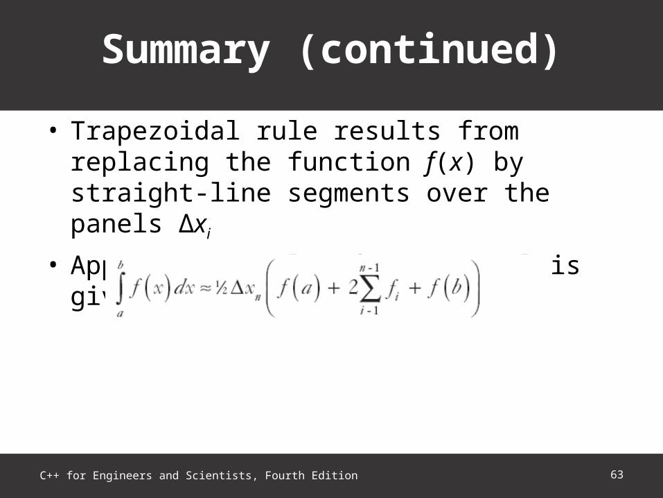
• Trapezoidal rule results from replacing the function f(x) by straight-line segments over the panels ∆xi
• Approximate value for integral is given by following formula
Summary (continued)
63C++ for Engineers and Scientists, Fourth Edition
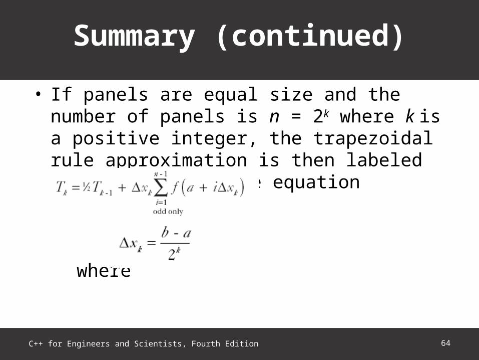
• If panels are equal size and the number of panels is n = 2k where k is a positive integer, the trapezoidal rule approximation is then labeled Tk and satisfies the equation
where
Summary (continued)
64C++ for Engineers and Scientists, Fourth Edition
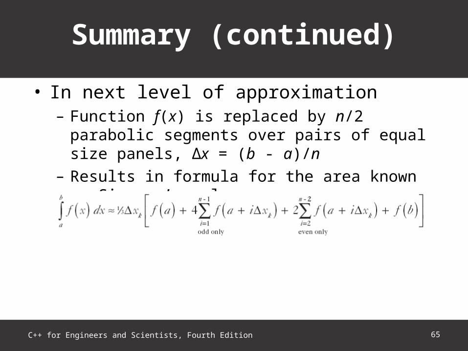
• In next level of approximation– Function f(x) is replaced by n/2 parabolic segments over
pairs of equal size panels, ∆x = (b - a)/n – Results in formula for the area known as Simpson’s rule:
Summary (continued)
65C++ for Engineers and Scientists, Fourth Edition


![Communication Skills [CMS] - diplomadiploma.vidyalankar.org/wp-content/uploads/Comp.pdfTopic 3 Numerical Method 3.1 Solution of algebraic equation ... • Bisection method • Regula](https://static.documents.pub/doc/80x56/5abd06607f8b9a76038e9f37/communication-skills-cms-3-numerical-method-31-solution-of-algebraic-equation.jpg)


![Extension of the SPEEDUP Path Integral Monte Carlo Code*parallel.bas.bg/dpa/IMACS_MCM_2011/Talks/Dusan...Bisection method Bisection method [2/2] Numbers from the Gaussian centered](https://static.documents.pub/doc/80x56/60f894a5813c9c6e2362fb35/extension-of-the-speedup-path-integral-monte-carlo-code-bisection-method-bisection.jpg)


