CHAPTER 15B 1 Chapter 15B Statistical Thermodynamics 2: Applications I. Fundamental Thermodynamic Relationships. A. Connection of the Partition Function with Thermodynamic Quantities. 1. Virtually every thermodynamic variable can be expressed in terms of the partition function Q from statistical mechanics. This is the bridge that connects the microscopic world with the macroscopic world of thermodynamics. Therefore, the central task of statistical mechanics is to derive the partition function for the system of interest, because the thermodynamics of the system can then be derived from Q. 2. We already saw this with thermodynamic internal energy U and entropy S. U = U( 0 ) − ∂ ln Q ∂β % & ' ( ) * V fixed or U = U( 0 ) + k B T 2 ∂ ln Q ∂T % & ' ( ) * V . fixed and S = U − U( 0 ) T + k B ln Q 3. Now through similar derivations we can write down all the important thermodynamic state functions in terms of the partition function Q: Since Helmholtz free energy A = U - TS: A = A( 0 ) − k B T ln Q where A( 0 ) = U( 0 ) Now since pressure P = − ∂A ∂V $ % & ' ( ) T , N P = k B T ∂ ln Q ∂V # $ % & ' ( T Now since enthalpy H = U + PV H = H( 0 ) + k B T 2 ∂ ln Q ∂T # $ % & ' ( V + k B TV ∂ ln Q ∂V # $ % & ' ( T
A. Connection of the Partition Function with Thermodynamic Quantities. 1. Virtually every thermodynamic variable can be expressed in terms of
the partition function Q from statistical mechanics. This is the bridge that connects the microscopic world with the macroscopic world of thermodynamics. Therefore, the central task of statistical mechanics is to derive the partition function for the system of interest, because the thermodynamics of the system can then be derived from Q.
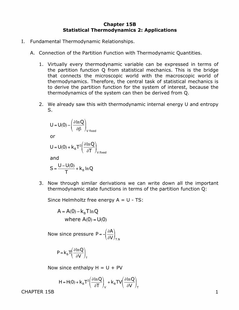
2. We already saw this with thermodynamic internal energy U and entropy
S.
€
U = U(0) − ∂lnQ∂β
%
& '
(
) *
V fixed
or
U = U(0) + kBT2 ∂lnQ
∂T%
& '
(
) *
V .fixed
and
S =U−U(0)
T+ kB lnQ
3. Now through similar derivations we can write down all the important
thermodynamic state functions in terms of the partition function Q: Since Helmholtz free energy A = U - TS:
€
A = A(0) −kBT lnQ where A(0) = U(0)
Now since pressure
€
P = −∂A∂V$
% &
'
( )
T ,N
€
P = kBT∂lnQ∂V
#
$ %
&
' (
T
Now since enthalpy H = U + PV
€
H = H(0) + kBT2 ∂lnQ
∂T#
$ %
&
' (
V
+ kBTV∂lnQ∂V
#
$ %
&
' (
T
CHAPTER 15B 2
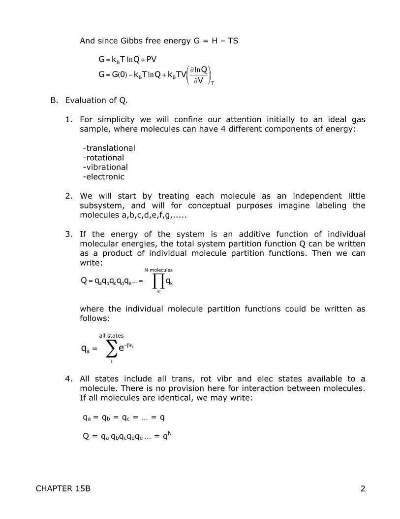
And since Gibbs free energy G = H – TS
€
G = kBT lnQ + PV
€
G = G(0) −kBT lnQ + kBTV∂lnQ∂V
$
% &
'
( )
T
B. Evaluation of Q.
1. For simplicity we will confine our attention initially to an ideal gas
sample, where molecules can have 4 different components of energy: -translational -rotational -vibrational -electronic 2. We will start by treating each molecule as an independent little
subsystem, and will for conceptual purposes imagine labeling the molecules a,b,c,d,e,f,g,.....
3. If the energy of the system is an additive function of individual
molecular energies, the total system partition function Q can be written as a product of individual molecule partition functions. Then we can write:
€
Q = qaqbqcqdqe...= qk
k
N molecules
∏
where the individual molecule partition functions could be written as
follows:
€
qa = e−βεi
i
all states
∑
4. All states include all trans, rot vibr and elec states available to a
molecule. There is no provision here for interaction between molecules. If all molecules are identical, we may write: qa = qb = qc = … = q Q = qa qbqcqdqe … = qN
CHAPTER 15B 3
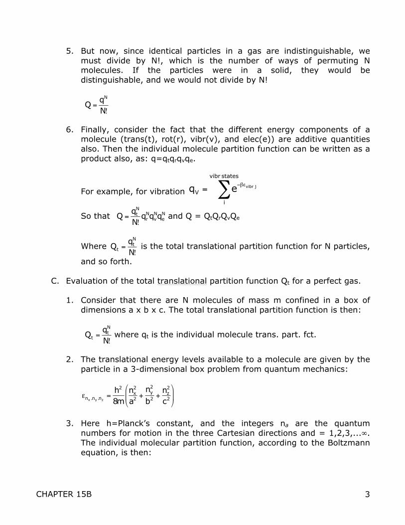
5. But now, since identical particles in a gas are indistinguishable, we
must divide by N!, which is the number of ways of permuting N molecules. If the particles were in a solid, they would be distinguishable, and we would not divide by N!
€
Q =qN
N!
6. Finally, consider the fact that the different energy components of a
molecule (trans(t), rot(r), vibr(v), and elec(e)) are additive quantities also. Then the individual molecule partition function can be written as a product also, as: q=qtqrqvqe.
For example, for vibration
€
qV = e−βεvibr j
i
vibr states
∑
So that
€
Q =qt
N
N!qr
NqvNqe
N and Q = QtQrQvQe
Where
€
Qt =qt
N
N! is the total translational partition function for N particles,
and so forth.
C. Evaluation of the total translational partition function Qt for a perfect gas. 1. Consider that there are N molecules of mass m confined in a box of
dimensions a x b x c. The total translational partition function is then:
€
Qt =qt
N
N! where qt is the individual molecule trans. part. fct.
2. The translational energy levels available to a molecule are given by the
particle in a 3-dimensional box problem from quantum mechanics:
€
εnx ,ny ,nz=
h2
8mnx
2
a2 +ny
2
b2 +nz
2
c2
#
$ %
&
' (
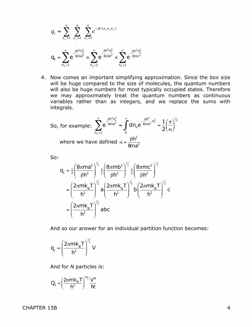
3. Here h=Planck’s constant, and the integers na are the quantum numbers for motion in the three Cartesian directions and = 1,2,3,...∞. The individual molecular partition function, according to the Boltzmann equation, is then:
CHAPTER 15B 4
∑∑∑∞
=
−∞
=
∞
=
=1
)(
11 z
zyx
yx n
nnn
nnt eq βε
€
qt = e−βh2nx
2
8ma2
nx =1
∞
∑ × e−βh2ny
2
8mb2
ny =1
∞
∑ × e−βh2nz
2
8mc2
nz =1
∞
∑
4. Now comes an important simplifying approximation. Since the box size
will be huge compared to the size of molecules, the quantum numbers will also be huge numbers for most typically occupied states. Therefore we may approximately treat the quantum numbers as continuous variables rather than as integers, and we replace the sums with integrals.
So, for example:
€
e−βh2nx
2
8ma2
nx =1
∞
∑ ≈ dnx
0
∞
∫ e−βh2
8ma2nx
2
=12
πα
*
+ ,
-
. /
12
where we have defined
€
α =βh2
8ma2
So:
qt= 12
8πma2
βh2#
$%%
&
'((
12
12
8πmb2
βh2#
$%%
&
'((
12
12
8πmc2
βh2#
$%%
&
'((
12
=2πmk
BT
h2
#
$%%
&
'((
12
a2πmk
BT
h2
#
$%%
&
'((
12
b2πmk
BT
h2
#
$%%
&
'((
12
c
=2πmk
BT
h2
#
$%%
&
'((
32
abc
And so our answer for an individual partition function becomes:
qt=2πmk
BT
h2
"
#$$
%
&''
32
V
And for N particles is:
€
Qt =2πmkBT
h2
#
$ %
&
' (
3N2 VN
N!
CHAPTER 15B 5
D. Thermodynamics of an Ideal Monatomic Gas.
1. Now that we have the translational partition function, we are ready to
discuss the thermal properties of an ideal monatomic gas. A monatomic gas has only translational and electronic energy, and we can ordinarily neglect the electronic component except at very high temperatures. (All molecules in ground electronic state, so no energy is being stored in electronic. Our starting point is the total translational partition function we derived previously:
€
Qt =2πmkBT
h2
#
$ %
&
' (
3N2 VN
N!
2. We want to derive the pressure of the gas, so we begin with the pressure equation we wrote down earlier:
€
P = kBT∂ lnQt
∂V#
$ %
&
' (
T ,N
ln Qt = ln C + N ln V where we have defined
€
C =2πmkBT
h2
#
$ %
&
' (
3N2 1N!
€
∂lnQt
∂V= N
∂lnV∂V
=NV
And thus:
€
P =NV
kBT which rearranges to the ideal gas equation:
€
PV = NkBT = nRT
Wow, we just derived the ideal gas law (and hence Boyle’s, Charles’ and Avogadro’s Law) starting with the particle in a box. (That is the power of statistical mechanics.)
3. Now, let’s derive the thermodynamics internal energy U of the
monatomic gas. From a previous result we found that U could be related to the partition function as follows (U(0)=0 since there is no vibrational zero-point energy):
€
U = kBT2 ∂lnQt
∂T#
$ %
&
' (
V ,N
CHAPTER 15B 6
€
U = kBT2 ∂∂T
3N2lnT
#
$ % &
' ( = kBT
2 3N2×
1T
; where we’ve defined
€
B ≡2πmkB
h2
$
% &
'
( )
3N2 VN
N!
€
U = kBT2∂ lnB+ lnT
3N2[ ]
∂T
#
$
% %
&
'
( (
And our final result is:
€
U =32
NkBT
4. Let’s analyze this result. It says the internal energy of a gas depends
only on two things: (1) the number of gas molecules (since the energy is an additive quantity, the sum of the energies of the individual molecules), and (2) the temperature. Doesn’t depend on the mass.
5. The result agrees with the classical equipartition theorem, which states
that: average energy stored in every degree of freedom of every molecule =
€
12
kBT
Since there are three degrees of translational freedom (and no other degrees, such as rotation or vibration), there are 3/2 kBT for every molecule.
6. The translational contribution to the constant volume heat capacity is computed as:
CVtrans =
∂Ut
∂T
"
#$$
%
&''V
CVtrans =
∂ 3 2( )NkBT∂T
"
#
$$
%
&
''V
= 3 2( )NkB ∂T∂T
"
#$$
%
&''V
= 3 2( )NkB
or: CVtrans = 3 2( ) R ; for one mole of gas.
CHAPTER 15B 7
E. Rotational Contribution to Thermodynamics of Gases. 1. Remember the total partition function can be written as a product of
four parts: Q = QtQrQvQe 2. where now we are interested in the rotation component Qr, which can
be written in terms of the single molecule rotational partition function qr as:
€
Qr = qrN; where N is the number of molecules in the system.
€
qr = e−βεi
i
states
∑ ; but using the degeneracy WJ, we could write:
€
qr = ΩJe−βεJ
J
levels
∑
3. Lets confine ourselves to a diatomic molecule. The energy levels and the degeneracy of a rigid diatomic rotor, from quantum mechanics, are given by the equations:
€
εJ =J J+1( )2
2I; J + 0,1,2…
€
ΩJ = 2J+1; so
€
qr = 2J+1( )J=0
∞
∑ e−β2J J+1( ) /2I
4. At this point it becomes useful to define a quantity called the “rotation
temperature” of the molecule. This is simply a collection of constants in the exponent of the previous equation.
€
θr ≡ 2 2IkB
5. The loose interpretation of θr is the temperature at which rotational
levels become appreciably populated. For example, θr = 9.4 K for HCl. Thus we see how easy it is for a system at room temperature to populate excited rotational levels.
6. We are trying to get a very simple expression for the partition function,
something simpler than the infinite sum we have above. In order to do this we can take advantage of the classical approximation. We
CHAPTER 15B 8
recognize that at room temperature, when qr <<T, the spacings between rotational levels is very small compared to typical thermal energies, such as kBT. When this is true, the rotor behaves as a classical rotor, rather than by quantum mechanics. Quantum rotational effects are no longer important at room temperature, in other words. The sum over J values can be replaced by an integral:
€
qr = dJ 2J+1( )e−β2J J+1( ) /2I
J=0
∞
∫
€
qr =Tσθr
7. Here we have made one minor addition, the division by the symmetry
correction factor σ, which = 2 for homonuclear diatomics such as N2 and = 1 for heteronuclear diatomics. It is also convenient to write qr in terms of the spectroscopic rotation constant B (cm-1).
€
B ≡
4πIc; c = speed of light, so that:
θr=BhckB
€
qr =kBTσhcB
8. Now we are in a position to evaluate various thermodynamics
quantities involving the rotational contribution. Let’s first evaluate the rotation contribution to the internal energy; we’ll call it Ur. This can be determined by evaluating the following partial differential expression:
€
Ur = kBT2 ∂lnQr
∂T#
$ %
&
' (
V ,N
; where ln Qr = N ln qr
€
Ur = kBT2 ∂∂T
N ln Tσθr
Ur = NkBT2 ×
1T&
' (
)
* +
Ur = NkBT
CHAPTER 15B 9
9. Again this verifies the classical equipartition theorem, which states that a molecule will on the average possess (1/2)kBT energy for every degree of freedom. A diatomic has two rotational degrees of freedom.
10. Now let us evaluate the rotational contribution to the constant volume
heat capacity, which is obtained by taking the partial derivative of the energy expression with respect to T at fixed volume:
€
CVrot =
∂Ur
∂T#
$ %
&
' (
V
CVrot =
∂NkBT∂T
#
$ %
&
' (
V
= NkB∂T∂T#
$ %
&
' (
V
= NkB
or:
€
CVrot = R; for one mole of gas.
F. Vibrational Contribution to Thermodynamics Properties of Gases.
1. Now we are ready to look at the vibrational contribution. Let us take
the simple diatomic molecule for example, which has a single vibrational mode of motion, which is bond-stretching. The quantum energy levels of vibration of a diatomic in the harmonic oscillator approximation are given by:
εv = (v + 1/2)hν; (v = 0,1,2,…∞) where ν is the oscillator frequency given by:
€
ν =12π
kµ
2. Here, k is the bond force constant and µ is the reduced mass of the
diatomic. Notice that the harmonic oscillator energy levels are evenly spaced with an energy gap between quantum states of hν and that there is no degeneracy. Also notice that the lowest possible energy is not zero, but a residual energy value of (1/2)hν.
3. We have already evaluated the vibrational partition function in the
harmonic oscillator approximation:
€
Qv = qvN
qv = e−β v+ 1
2( )hνv=0∑
qv = e−βhν
2 e−βvhν
v=0∑
CHAPTER 15B 10
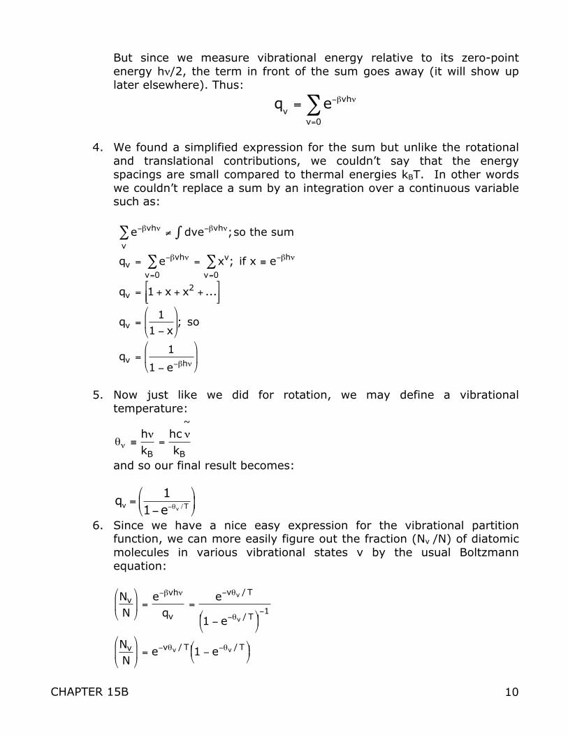
But since we measure vibrational energy relative to its zero-point energy hν/2, the term in front of the sum goes away (it will show up later elsewhere). Thus:
qv= e−βvhν
v=0
∑
4. We found a simplified expression for the sum but unlike the rotational and translational contributions, we couldn’t say that the energy spacings are small compared to thermal energies kBT. In other words we couldn’t replace a sum by an integration over a continuous variable such as:
€
e−βvhν
v∑ ≠ dve−βvhν;so the sum∫
qv = e−βvhν
v=0∑ = xv
v=0∑ ; if x ≡ e−βhν
qv = 1 + x + x2 + ...) * +
, - .
qv =1
1 − x
/
0 1
2
3 4 ; so
qv =1
1 − e−βhν
/
0 1
2
3 4
5. Now just like we did for rotation, we may define a vibrational
temperature:
€
θν ≡hνkB
=hc ν
~
kB and so our final result becomes:
€
qv =1
1−e−θv /T
$
% &
'
( )
6. Since we have a nice easy expression for the vibrational partition function, we can more easily figure out the fraction (Nv /N) of diatomic molecules in various vibrational states v by the usual Boltzmann equation:
€
Nv
N
"
# $
%
& ' =
e−βvhν
qv=
e−vθv / T
1 − e−θv / T" # $ %
& ' −1
Nv
N
"
# $
%
& ' = e−vθv / T 1 − e−θv / T"
# $ %
& '
CHAPTER 15B 11
G. Electronic Contributions to the Partition Function. 1. The individual molecule electronic state partition function for an
arbitrary molecule can be written simply as a sum of the Boltzmann factor over electronic energy levels, times the degeneracy of the levels:
qe= Ω
nn
elec levels
∑ e−βεn
2. Contrary to the text, it is usual to measure molecular electronic energy
relative to the energy of dissociated atoms, which is called the zero of energy. Here is a schematic electronic energy level diagram as a function of the internuclear distance r, showing two electronic energy surfaces:
3. The energy of the ground state is thus ε1 = -Do, and the first excited
state is:
ε2 = -Do +Δ1. 4. The electronic partition function can thus be simply written as:
€
qe =ΩoeβDo +Ω1e
β Do −Δ1( )
qe = eβDo Ωo +Ω1e−βΔ1( )
CHAPTER 15B 12
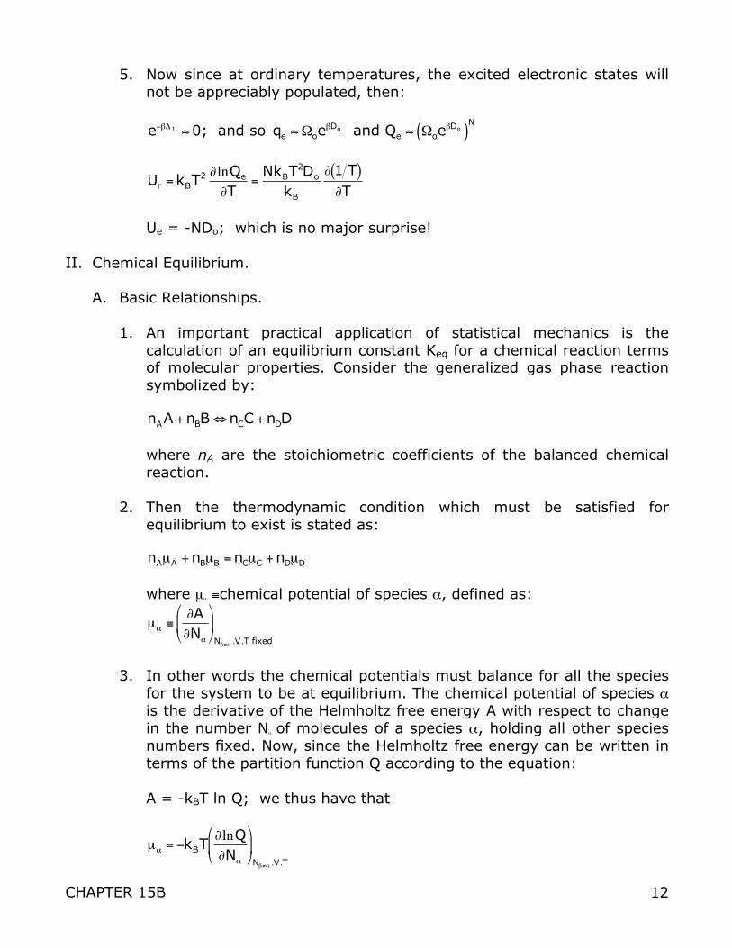
5. Now since at ordinary temperatures, the excited electronic states will not be appreciably populated, then:
€
e−βΔ1 ≈0; and so
€
qe ≈ ΩoeβDo and Qe ≈ Ωoe
βDo( )N
€
Ur = kBT2 ∂lnQe
∂T=
NkBT2Do
kB
∂ 1 T( )∂T
Ue = -NDo; which is no major surprise!
II. Chemical Equilibrium.
A. Basic Relationships.
1. An important practical application of statistical mechanics is the calculation of an equilibrium constant Keq for a chemical reaction terms of molecular properties. Consider the generalized gas phase reaction symbolized by:
€
nAA + nBB⇔nCC + nDD where nA are the stoichiometric coefficients of the balanced chemical
reaction. 2. Then the thermodynamic condition which must be satisfied for
equilibrium to exist is stated as:
€
nAµA + nBµB = nCµC + nDµD where µα ≡chemical potential of species α, defined as:
€
µα ≡∂A∂Nα
%
& '
(
) * Nβ≠α ,V ,T fixed
3. In other words the chemical potentials must balance for all the species
for the system to be at equilibrium. The chemical potential of species α is the derivative of the Helmholtz free energy A with respect to change in the number Nα of molecules of a species α, holding all other species numbers fixed. Now, since the Helmholtz free energy can be written in terms of the partition function Q according to the equation:
A = -kBT ln Q; we thus have that
€
µα = −kBT∂lnQ∂Nα
%
& '
(
) * Nβ≠α ,V ,T
CHAPTER 15B 13
4. Now, if the species A, B, C, D are independent particles and
distinguishable, the total partition function Q for the entire mixture is:
€
Q = QAQBQCQD =qA
NA
NA!qB
NB
NB!qC
NC
NC!qD
ND
ND!
∂lnQ∂Nα
= ln qα
Nα
$
% &
'
( )
or µA = −kBTqα
Nα
$
% &
'
( )
Q = QAQ
BQ
CQ
D=
qA
NA
NA!
qB
NB
NB!
qC
NC
NC!
qD
ND
ND!
∂lnQ∂N
α
= lnqα
Nα
#
$%%
&
'((
or µA= −k
BT
qα
Nα
#
$%%
&
'((
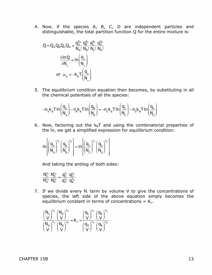
5. The equilibrium condition equation then becomes, by substituting in all
the chemical potentials of all the species:
−nAkBT ln
qA
NA
"
#$$
%
&'' −nBkBT ln
qB
NB
"
#$$
%
&'' = −nCkBT ln
qC
NC
"
#$$
%
&'' −nDkBT ln
qD
ND
"
#$$
%
&''
6. Now, factoring out the kBT and using the combinatorial properties of
the ln, we get a simplified expression for equilibrium condition:
lnqA
NA
!
"##
$
%&&
nAqB
NB
!
"##
$
%&&
nB'
(
)))
*
+
,,,= ln
qC
NC
!
"##
$
%&&
nCqD
ND
!
"##
$
%&&
nD'
(
)))
*
+
,,,
And taking the antilog of both sides:
€
NCnc
NAnA
NDnD
NBnB
=qC
nc
qAnA
qDnD
qBnB
7. If we divide every Nα term by volume V to give the concentrations of species, the left side of the above equation simply becomes the equilibrium constant in terms of concentrations = Kc.
€
NC
V"
# $
%
& ' nC
NA
V"
# $
%
& ' nA
ND
V"
# $
%
& ' nD
NB
V"
# $
%
& ' nB
= Kc =
qC
V"
# $
%
& ' nC
qA
V"
# $
%
& ' nA
qD
V"
# $
%
& ' nD
qB
V"
# $
%
& ' nB
CHAPTER 15B 14
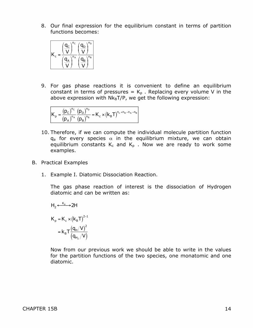
8. Our final expression for the equilibrium constant in terms of partition functions becomes:
€
Kc =
qC
V"
# $
%
& ' nC
qA
V"
# $
%
& ' nA
qD
V"
# $
%
& ' nD
qB
V"
# $
%
& ' nB
9. For gas phase reactions it is convenient to define an equilibrium
constant in terms of pressures = Kp . Replacing every volume V in the above expression with NkBT/P, we get the following expression:
€
Kp =pC( )nC
pA( )nA
pD( )nD
pB( )nB= Kc × kBT( )nc +nD−nA −nB
10. Therefore, if we can compute the individual molecule partition function
qa for every species α in the equilibrium mixture, we can obtain equilibrium constants Kc and Kp . Now we are ready to work some examples.
B. Practical Examples
1. Example I. Diatomic Dissociation Reaction. The gas phase reaction of interest is the dissociation of Hydrogen
diatomic and can be written as:
€
H2Kp← → $ 2H
€
Kp = Kc × kBT( )2−1
= kBTqH V( )2
qH2V( )
Now from our previous work we should be able to write in the values
for the partition functions of the two species, one monatomic and one diatomic.
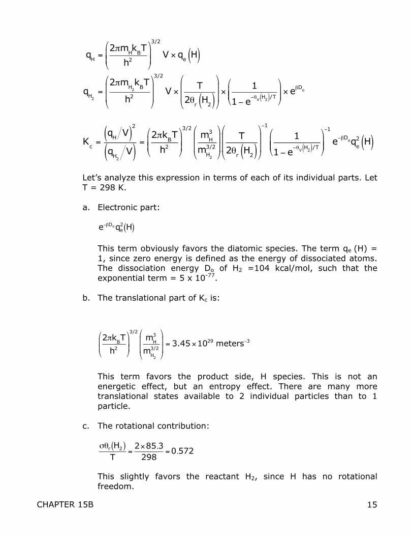
CHAPTER 15B 15
qH=2πm
HkBT
h2
"
#$$
%
&''
3/2
V × qeH( )
qH2=2πm
H2kBT
h2
"
#
$$
%
&
''
3/2
V × T
2θrH2( )
"
#
$$
%
&
'' ×
1
1− e−θV H2( )/T
"
#$$
%
&'' × e
βDo
Kc=qHV( )2
qH2V( )
=2πk
BT
h2
"
#$$
%
&''
3/2mH3
mH2
3/2
"
#
$$
%
&
''
T
2θrH2( )
"
#
$$
%
&
''
−1
1
1− e−θV H2( )/T
"
#$$
%
&''
−1
e−βDoqe2 H( )
Let’s analyze this expression in terms of each of its individual parts. Let
T = 298 K.
a. Electronic part:
€
e−βDoqe2 H( )
This term obviously favors the diatomic species. The term qe (H) = 1, since zero energy is defined as the energy of dissociated atoms. The dissociation energy Do of H2 =104 kcal/mol, such that the exponential term = 5 x 10-77.
b. The translational part of Kc is:
2πkBT
h2
"
#$$
%
&''
3/2mH3
mH2
3/2
"
#
$$
%
&
'' = 3.45 ×10
29 meters−3
This term favors the product side, H species. This is not an energetic effect, but an entropy effect. There are many more translational states available to 2 individual particles than to 1 particle.
c. The rotational contribution:
€
σθr H2( )T
=2×85.3
298= 0.572
This slightly favors the reactant H2, since H has no rotational
freedom.
CHAPTER 15B 16
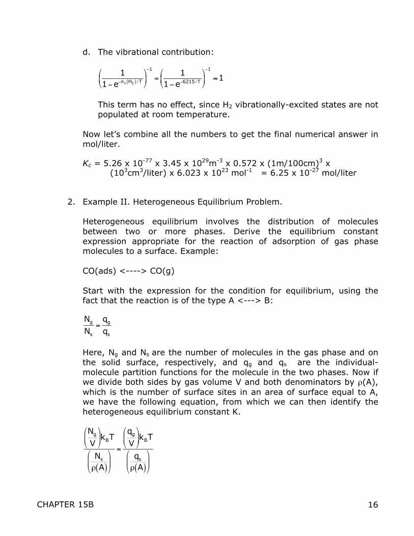
d. The vibrational contribution:
€
11−e−θv H2( ) /T
$
% &
'
( ) −1
=1
1−e−6215 /T
$
% &
'
( ) −1
≈1
This term has no effect, since H2 vibrationally-excited states are not
populated at room temperature. Now let’s combine all the numbers to get the final numerical answer in
mol/liter. Kc = 5.26 x 10-77 x 3.45 x 1029m-3 x 0.572 x (1m/100cm)3 x (103cm3/liter) x 6.023 x 10²³ mol-1 = 6.25 x 10⁻²⁷ mol/liter 2. Example II. Heterogeneous Equilibrium Problem. Heterogeneous equilibrium involves the distribution of molecules
between two or more phases. Derive the equilibrium constant expression appropriate for the reaction of adsorption of gas phase molecules to a surface. Example:
CO(ads) <----> CO(g) Start with the expression for the condition for equilibrium, using the
fact that the reaction is of the type A <---> B:
€
Ng
Ns
=qg
qs
Here, Ng and Ns are the number of molecules in the gas phase and on the solid surface, respectively, and qg and qs are the individual-molecule partition functions for the molecule in the two phases. Now if we divide both sides by gas volume V and both denominators by ρ(A), which is the number of surface sites in an area of surface equal to A, we have the following equation, from which we can then identify the heterogeneous equilibrium constant K.
€
Ng
V
"
# $
%
& ' kBT
Ns
ρ A( )
"
# $
%
& '
=
qg
V
"
# $
%
& ' kBT
qs
ρ A( )
"
# $
%
& '
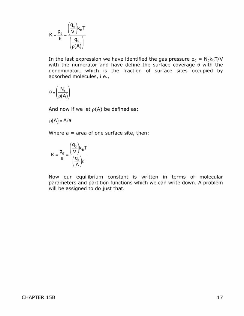
CHAPTER 15B 17
€
K =pg
θ=
qg
V
#
$ %
&
' ( kBT
qs
ρ A( )
#
$ %
&
' (
In the last expression we have identified the gas pressure pg = NgkBT/V
with the numerator and have define the surface coverage θ with the denominator, which is the fraction of surface sites occupied by adsorbed molecules, i.e.,
€
θ ≡Ns
ρ A( )
%
& '
(
) *
And now if we let ρ(A) be defined as:
€
ρ A( ) = A a
Where a = area of one surface site, then:
€
K =pg
θ=
qg
V
#
$ %
&
' ( kBT
qs
A#
$ %
&
' ( a
Now our equilibrium constant is written in terms of molecular
parameters and partition functions which we can write down. A problem will be assigned to do just that.