EPA/600/R-99/030 * Corresponding author address: Gerald L. Gipson, MD-80, Research Triangle Park, NC 27711. E-mail: [email protected]Chapter 16 PROCESS ANALYSIS Gerald L. Gipson * Human Exposure and Atmospheric Sciences Division National Exposure Research Laboratory U. S. Environmental Protection Agency Research Triangle Park, NC 27711 ABSTRACT The implementation of process analysis techniques in the Models-3 Community Multiscale Air Quality (CMAQ) modeling system is described in this chapter. These techniques can be used in Eulerian photochemical models such as the CMAQ Chemical Transport Model (CCTM) to obtain information that provides insights into how model predictions are obtained. This type of information is particularly useful when modeling nonlinear systems such as atmospheric photochemistry. The two techniques available in the CMAQ system – integrated process rate (IPR) analysis and integrated reaction rate analysis (IRR) -- are each described. The manner in which IPR analysis can be used to determine the relative contributions of individual physical and chemical processes is presented. Descriptions of how to employ IRR analysis to elucidate important chemical pathways and to identify key chemical characteristics are included. Finally, the procedures used to apply each technique in the CMAQ system are also described.
Transcript
EPA/600/R-99/030
*Corresponding author address: Gerald L. Gipson, MD-80, Research Triangle Park, NC 27711. E-mail:[email protected]
Chapter 16
PROCESS ANALYSIS
Gerald L. Gipson*
Human Exposure and Atmospheric Sciences DivisionNational Exposure Research LaboratoryU. S. Environmental Protection Agency
Research Triangle Park, NC 27711
ABSTRACT
The implementation of process analysis techniques in the Models-3 Community Multiscale AirQuality (CMAQ) modeling system is described in this chapter. These techniques can be used inEulerian photochemical models such as the CMAQ Chemical Transport Model (CCTM) to obtaininformation that provides insights into how model predictions are obtained. This type ofinformation is particularly useful when modeling nonlinear systems such as atmosphericphotochemistry. The two techniques available in the CMAQ system – integrated process rate(IPR) analysis and integrated reaction rate analysis (IRR) -- are each described. The manner inwhich IPR analysis can be used to determine the relative contributions of individual physical andchemical processes is presented. Descriptions of how to employ IRR analysis to elucidateimportant chemical pathways and to identify key chemical characteristics are included. Finally,the procedures used to apply each technique in the CMAQ system are also described.
EPA/600/R-99/030
16-1
16.0 PROCESS ANALYSIS
A major function of air pollution models is to predict the spatial and temporal distributions ofambient air pollutants and other species. For complex Eulerian grid models, output concentrationfields of these species are determined by solving systems of partial differential equations. Theseequations define the time-rate of change in species concentrations due to a series of physical andchemical processes (e.g., emissions, chemical reaction, horizontal advection, etc.). Since mostgrid models are configured to output only the concentration fields that reflect the cumulativeeffect of all processes, information about the impact of individual processes is usually notavailable. Grid models can be configured to provide quantitative information on the effects of the chemical reactions and other atmospheric processes that are being simulated, however(Pleim, 1990; Jeffries and Tonnesen, 1994; Jang et al., 1995a,b). This type of information hasbeen used to develop various process analyses that provide descriptions of how a model obtainedits predictions. This chapter provides background information on these methods and describeshow process analysis is implemented in the Models-3 Community Multiscale Air Quality(CMAQ) modeling system.
Although process analysis does not have to be included in a grid model application, it can providesupplemental information that can be quite useful in assessing a model's performance. Quantifying the contributions of individual processes to model predictions provides afundamental explanation of the reasons for a model's predictions and shows the relativeimportance of each process. This information can be useful in identifying potential sources oferror in the model formulation or its inputs. It can also be useful in interpreting model outputs,particularly with respect to understanding differences in model predictions that occur from achange to the model itself or to its input. Further, information provided from the chemicalprocess analysis can be used to determine important characteristics of different chemicalmechanisms. This is particularly useful for investigating mechanistic differences under differentchemical regimes (e.g., VOC versus NOx limiting conditions).
The inclusion of process analysis in a model application is generally carried out in two steps. First, the model itself is “instrumented” (i.e., additional code or modules are added to the model)to produce supplemental outputs about the contributions of individual processes and differentchemical reaction pathways to the model predictions. These data are then used with theconcentration fields in postprocessing operations to provide quantitative explanations of thefactors affecting a model's predictions. Although several specific postprocessing techniques havebeen developed to reveal particular model features (e.g., Jeffries and Tonnesen, 1994; Jang et al.,1995a,b), process analysis data can be extracted and analyzed in many different ways. Theimplementation of process analysis in the CMAQ system has been structured to facilitate dataextraction for subsequent model analysis. Although the main focus of this chapter is on dataextraction techniques, some example process analyses are also presented to illustrate particularapplications.
For purposes of discussion, it is convenient to separate process analysis into two parts: integratedprocess rate (IPR) analysis and integrated reaction rate (IRR) analysis. The first deals with the
EPA/600/R-99/030
16-2
effects of all the physical processes and the net effect of chemistry on model predictions. IRRanalysis deals with the details of the chemical transformations that are described in the model'schemical mechanism. In general, IPR analyses are generally much easier to apply and understandthan IRR analyses since the latter typically requires a fairly thorough understanding ofatmospheric chemistry. Thus, the discussion below describes each analysis method separately,starting with IPR analyses. Users not familiar with atmospheric chemistry details may wish toomit the sections on IRR analysis. It should be added that either analysis method can be appliedindependently of the other.
The CMAQ implementation of process analysis includes a flexible user interface that allows theuser to request only those particular outputs that are needed for model analysis. The informationgenerated for both IPR analysis and IRR analysis is controlled by the Process Analysis ControlProgram (PACP). The PACP processes user-specified commands to instrument the CMAQChemical Transport Model (hereafter referred to as the CCTM) to generate the specific outputsthat are selected by the user. As a consequence, the PACP must be invoked before configuring aCCTM and running a simulation. The details of how the PACP works and the syntax for thecommands are covered in the Models-3 User Manual (EPA, 1998), and they will not be repeatedin their entirety here. Nevertheless, some of the command syntax and some simple examples arepresented in the discussions that follow to illustrate how the PACP is used to set up a particularprocess analysis.
16.1 Integrated Process Rate Analysis
The governing equation for Eulerian models is the species continuity equation. Application ofthe continuity equation to a group of chemically reactive species results in a system of partialdifferential equations (PDEs) that gives the time-rate of change in species concentration as afunction of the rates of change due to various chemical and physical processes that determine theambient species concentrations. As noted in the introduction, the concentration fields that arethe numerical solutions to these PDEs reveal only the net effects of all processes. This section isconcerned with how the contributions of individual processes are determined and used in processanalyses. The first two subsections deal with the calculation and use of IPRs in general. The lasttwo subsections describe the CMAQ implementation of IPR analysis and the use of the PACP toset up an IPR analysis.
16.1.1 Computation of Integrated Process Rates
All Eulerian models utilize the technique of operator splitting. As a result, it is relatively easy toobtain quantitative information about the contribution of individual processes to totalconcentrations. In operator splitting, solutions to the system of PDEs are obtained by separatingthe continuity equation for each species into several simpler PDEs or ordinary differentialequations (ODEs) that give the impact of only one or two processes. These simpler PDEs orODEs are then solved separately to arrive at the final concentration. To illustrate, consider thesimple case of two-dimensional horizontal advection of a single species in the absence of anyother processes, for which the governing equation can be expressed as follows:
EPA/600/R-99/030
16-3
0c0t
�0(uc)0x
�0(vc)0y
0 , (16-1)
where c is the species concentration, and u and v are the x- and y-components of the windvelocity vector, respectively. With operator splitting, this 2-dimensional equation is split into two1-dimensional operators, one for each direction:
0c0t
�0(uc)0x
0 (16-2a)
and
0c0t
�0(vc)0y
0 . (16-2b)
These two equations are then solved sequentially, with the solution to the first being used as theinitial condition for the second. The solution to the second equation then represents the finalsolution and gives the net effect of 2-dimensional advection.
The final solution for the example presented above can also be represented as follows:
c(t ��t) c(t) � (�c)x � (�c)y, (16-3)
where c(t+�t) is the final solution, c(t) is the initial condition for the 2-dimensional problem, and(�c)x and (�c)y are the changes in concentration produced by each of the 1-dimensionaloperators. (�c)x and (�c)y give the impact of each operator in moving from the initial to the finalconcentration and are equivalent to the results obtained by integrating the process ratesindividually. Hence the term integrated process rates is used to describe them. Note that theycan be computed with little additional work since they are simply equal to the difference betweenthe final and initial concentrations for each operator.
From the above example, it should be evident that a general mathematical representation of IPRsfor individual processes can be expressed as follows:
(�c)n Pt��t
tLn dt , (16-4)
where (�c)n is the change in a species' concentration due to operator n, Ln is the differentialoperator associated with a process, and �t is the model synchronization time step (which isequivalent to �tsync in Chapter 6). Refer to Chapter 6 for a discussion of the various time stepsused in CMAQ. The integration in equation (16-4) is performed by the model regardless ofwhether it has been instrumented for process analysis. Thus, it is only necessary to save the(�c)n to obtain process analysis capabilities. In a few cases, however, models may be structuredsuch that one operator deals with two or three processes simultaneously. In those cases, the
EPA/600/R-99/030
16-4
(�c)n obtained after the integration would represent the compound effect of all of thoseprocesses and it would not be possible to discern the impacts of the individual processes. Normally, the only way that information could be obtained would be to integrate the processrates separately. In some instances, however, it may still be possible to isolate the impacts of theindividual processes without performing additional integrations. For example, the CCTM treatsvertical diffusion, emissions, and dry deposition simultaneously in one operator, but the amountof material deposited by dry deposition is tabulated and the amount of material that is emitted isknown. As a consequence, mass balance techniques can be used to compute the contribution ofeach process subsequent to the simultaneous integration of the process rates without separatelyintegrating each process rate. Thus, the IPRs that are available for process analysis are to somedegree determined by the underlying structure of the photochemical model that is being used andby the effort that is invested in separating individual components when processes are coupled ina single operator.
Analogous to equation (16-3), the concentration at the end of a time step can be expressed asfollows:
c(t��t) c(t) �MN
n1
(�c)n, (16-5)
where the model is assumed to have N operators. It should be noted that most IPRs can be eitherpositive or negative since most processes can cause concentrations to either increase or decrease. Further, it should also be evident that the IPRs in the above expression are additive. Thus, forexample, the IPRs for horizontal advection and vertical advection could be summed to give oneIPR that represents the net impact of the two advection processes. The differential operators (Ln)themselves are most often nonlinear, however. Because of these nonlinearities, the magnitude ofthe IPRs for most processes would change if the order of the model’s operators was altered oreven if only one of the operators was changed. Thus, the additive property for IPRs holds onlyfor a particular application of the model.
16.1.2 Example IPR Analyses
The tabulation and subsequent output of IPRs provide the user with quantitative information onthe effects of individual processes, and these can be examined and depicted in a number ofways. Figures 16-1 and 16-2 contain two types of displays that were developed to depict processcontribution data graphically (Jeffries, 1996). Figure 16-1 is a time series plot showing bothpredicted concentrations and integrated process rates. This type of plot shows the hourlyvariations at a cell (or group of cells if the data are aggregated) of a predicted speciesconcentration and the change in concentration caused by each process (i.e., the IPRs). Plots ofthis type illustrate the variations in process contributions during the simulation period. Figure 16-2 shows process contributions and total concentrations for different model formulations, in thiscase, different grid resolutions. Here the data have been aggregated over several cells and hours,but could be developed for a single cell or time period just as well. This figure highlights howcumulative process contributions are altered by the different model formulations. For a more
EPA/600/R-99/030
16-5
thorough discussion of how this type of data can be used to assist in the evaluation of a model'sperformance, the reader is referred to Jang et al. (1995a and 1995b) and to Pleim (1990).
16.1.3 Implementation of IPR Analysis in the CMAQ System
The previous section illustrated that instrumenting a model for process analysis involvesproviding the capability to capture IPRs. Since an IPR can be calculated for every combinationof process and species, the amount of output data that can be generated is substantial. As aconsequence, the PACP has been designed to allow substantial flexibility in selecting theparticular IPRs for output. This is accomplished primarily by allowing the user to choose onlythose particular species/process combinations that are of interest. Additional control andflexibility are provided by including the ability to produce lumped IPRs, by allowing specialspecies families to be defined, and by providing controls to limit the size of the modeling domainfor which outputs are generated. These will be illustrated in the examples presented below.
The physical processes that are simulated in the CCTM and hence are available for IPR analysisare shown in Table 16-1. As will be illustrated below, these processes are referenced in thePACP by the codes shown in the first column. The procedure for selecting specific IPRs foroutput is species oriented. Hence, a user selects a species and then indicates which processeswill be included in the IPR output. The species are referenced by their model names. Inaddition, the user may also define a family of species that is a linear combination of the modelspecies (e.g., defining NOx as the sum of NO and NO2) and extract IPRs for the family. This canbe useful in saving disk space occupied by the output IPR files when information aboutindividual members of a family is not needed.
It should be apparent from Table 16-1 that IPRs for some species will always be zero (e.g., thosespecies not emitted always have zero IPRs for that process). Thus, the size of the output file canbe minimized by not extracting those IPRs. The PACP also contains an option that allows theuser to limit the amount of output data by extracting IPR outputs for only part of the modelingdomain. Currently, the user is restricted to selecting a single, contiguous block of cells within thedomain for the IPR outputs. The block is defined relative to the modeling domain by selecting astarting and ending column, row and level. A possible future enhancement would be to provide agraphical interface to allow the user to select any particular cell or group of cells within thedomain.
The CCTM model has been instrumented to write the IPRs to an output file at the same time asthe output concentration files are written. Thus, the IPR outputs represent the cumulative impactof the process integrations over the entire output time interval. Process contributions overshorter time intervals can be obtained by increasing the frequency of writing outputs of both theconcentration fields and the IPRs. Finally, the IPR output files are standard Models-3 IO/APIgridded files, and can be viewed with the Models-3 visualization tools described in Models-3User Manual (EPA, 1998).
EPA/600/R-99/030
16-6
16.1.4 Use of the PACP to set up an IPR Analysis
This section illustrates how the PACP can be used to generate the IPR data for an analysis.Details on formatting inputs and using the PACP are contained in the Models-3 User Manual(EPA, 1998). This section borrows from that discussion to illustrate how the PACP is used. Theuser selects and controls the form of the IPR output data by means of a PACP command file. Afew predefined command files are available to set up an analysis, or users can generate their ownfiles to customize their analyses. A command file consists of a series of commands anddefinitions that contain instructions for generating IPR outputs. The commands are input in afree form format to facilitate encoding, and they contain special keywords that have specificmeaning to the PACP. The commands related to IPR analysis have been divided into twogroups: Global commands and IPR output commands. A description of the commands withineach group will be presented first, followed by an example illustrating how these commands areused. In the description that follows, the syntax for each command is given first, with bold typeused for PACP keywords and normal type used for user supplied input. Alternative inputs areseparated by vertical bars and completely optional inputs are enclosed in curly braces.
The OUTPUT_DOMAIN command provides the capability to limitthe IPR output data to only one portion of the modeling domain. The ni in brackets are numbers that define the bounds of the outputdomain relative to the number of columns, rows, and vertical levelsin the modeling domain. Thus, for example, the value for n1 mustbe greater than or equal to one and less than or equal to thenumber of columns in the domain. If this command is included, atleast one domain specifier must be present, and the end of thedomain is used for any that are missing. If the command is omittedentirely, output is generated for the entire domain.
The DEFINE FAMILY command is used to define a group ofspecies as members of a family. The user specified “familyname”must be unique, and can be referenced in subsequent commands. The ci are numerical coefficients that default to one if notspecified; “speciesi” are the names of individual model species.
EPA/600/R-99/030
16-7
ENDPA;
The ENDPA command signifies the end of the command input inthe PACP command file.
The IPR_OUTPUT command defines specific IPR outputs to begenerated during a CMAQ simulation. A species name, familyname, or the keyword ALL must follow the IRR_OUTPUTkeyword. The keyword ALL refers to all model species. IPRs are generated for the selected species or family, and they arecontrolled by the specified values of pcodei, where pcodeicorresponds to one of the process codes listed in Table 16-1. If noprocess codes are specified, IPRs will be generated for everyprocess. The output variables that are generated are named eitherspecies_pcodei or familyname_pcodei
A listing of an example PACP command file is contained in Exhibit 16-1. To facilitate thediscussion that follows, the commands have been numbered, although this is not required by thePACP. (Note that all information enclosed by curly braces in a command file is treated ascomments.) Each numbered line represents a command, and the input for each command isterminated by a semicolon. This particular set of commands causes the CCTM to generateseveral individual IPRs for a special user-defined sub-domain. Each of the commands isdescribed below.
Command 1 is used to restrict the process analysis output to a subset of the modeling domain. Asnoted above, output would be generated for the entire computational domain if theOUTPUT_DOMAIN were omitted. Since keywords for columns and rows are not present, thePACP default is to include all rows and columns in the modeling domain. The keywords“LOLEV” and “HILEV” restrict the output for the vertical level to layers 1 through 2. Thus, thenet effect of this command is to limit the IPR output to all cells within the first two vertical levelsof the modeling domain.
Commands 2 and 3 are used to define families of species. The species names to the right of theequal sign are model species. The effect of the numerical coefficients in the definition of theVOC families is to convert the units of the IPRs for individual organics from ppm to ppmC. Aswill be seen, these “defined” family names are referenced in subsequent commands.
Commands 4 through 8 actually cause IPR outputs to be generated. As described above, IPRsare generated for the species and the processes that are referenced by means of the codes listedin Table 16-1. Since no process codes are specified in commands 4 and 5, IPRs will be generated
EPA/600/R-99/030
16-8
for each of the twelve processes in Table 16-1 for the families NOX and VOC (i.e., a total of 24IPRs). Command 6 causes three IPRs to be generated for species O3, one each for totaltransport, chemistry, and clouds. Command 7 causes an IPR for vertical diffusion to begenerated for every model species. The last command signifies the end of the command inputs.
The CCTM will generate the IPR output data in a form comparable to the output concentrationfiles. Hence, the data are written to standard Models-3 IO/API gridded data files. The units ofthe IPR data are normally the same as those for the species concentration data (i.e., ppm for gas-phase species and either µg/m3 or number/m3 for aerosols). As described in the example ofcreating the family VOC with units of ppmC, however, different output units can be createdusing special family definitions.
The example just described was formulated primarily to illustrate how IPR commands arestructured to collect IPR information during a model simulation. In general, the particular datathat are collected for process analysis would be determined by the needs of the study, and thus itis difficult to define a “default” process analysis. Nevertheless, a minimal process analysis forstudying ozone formation might involve collecting the process contributions for NOx, VOC, andfor ozone. The example in Exhibit 16-1 could be used as the starting point for such an analysis. Commands 4 and 5 capture all the IPRs for NOx and VOC. Command 6 could be modified tocapture all IPRs for ozone as well. Since it would not normally be necessary to capture verticaldiffusion IPRs for all species, command 7 could be dropped. Of course, the user would still berequired to define the domain for outputs (command 1) and to define the VOC family for themechanism that is being used (command 3). Thus, commands 1 through 5 with command 6modified to collect all IPRs for ozone would provide some very basic process analysisinformation on the formatio of ozone during a simulation.
16.2 Integrated Reaction Rate Analysis
The second major component of process analysis is IRR analysis. It is applied to investigate gas-phase chemical transformations that are simulated in the model. Its primary use to date has beento help explain how ambient ozone is formed in the chemical mechanisms that are used inphotochemical models (e.g., Jeffries and Tonnesen, 1994; Tonnesen and Jeffries, 1994). Thus,the CMAQ implementation of IRR analysis currently addresses only gas-phase reactions. Nevertheless, the concepts should be adaptable to the modules simulating aerosol formation andaqueous chemistry as well, and this is an area for future enhancement in the CCTM. Theremainder of this section describes how the IRRs are calculated and generated in the CMAQsystem.
16.2.1 Computation of Integrated Reaction Rates
As described in Chapter 8, the simulation of atmospheric chemistry is a key component of aphotochemical air quality model. The operator splitting techniques that are used in Eulerianphotochemical models typically result in a set of nonlinear, coupled, ordinary differentialequations (ODEs) that describe chemical interactions in the gas-phase. Solutions to these ODEs
EPA/600/R-99/030
16-9
are obtained using numerical solvers to compute species concentrations as a function of time. Again, these computed concentrations show only the net effect of chemical transformations. Ashas been done for physical processes, a technique has been developed to provide quantitativeinformation on individual chemical transformations (Jeffries and Tonnesen, 1994). Since thetechnique involves integrating the rates of the individual chemical reaction, the method is termedintegrated reaction rate analysis.
As was noted in section 8.3.1, the mathematical expression for the rate of a chemical reactiontakes one of the forms of equation set 8-3. The reaction rate is used to compute the change inspecies concentration that is caused by the reaction. Mathematically, this can be expressed asfollows:
Ml (t��t) Ml (t) � Pt��t
tr l dt , (16-6)
where Ml refers to the integrated reaction rate (IRR) for reaction l, �t is the modelsynchronization time step used by the chemical solver, and r l is the rate of reaction lcorresponding to one of the forms of equation set 8-3. The value of Ml represents the totalthroughput of the reaction, and can be used with the appropriate stoichiometry to determine theamount of an individual species that is produced or consumed by the reaction. For example,assume the IRR for the reaction A + B � 2C is 20 ppb for a given time period. Then, the amountof A and B consumed in that time period by this reaction is 20 ppb, and correspondingly, theamount of C produced is 40 ppb. Further, the net change in a species concentration due to allchemical reactions is equivalent to the sum of all its production terms less the sum of all its lossterms. As a consequence, the contribution of each reaction to the change in concentration of anyspecies is directly available from the IRRs. With this information, it is possible to identify theimportant chemical pathways that affect species concentrations and thereby unravel the complexchemical interactions that are being simulated.
As described in Chapter 8-4, the chemistry solvers used in air quality models typically employmarching methods that compute species concentrations at the end of a time step given theconcentrations at the beginning of the step. Since the solvers adjust the time steps to maintainstability and accuracy, the reaction rates should not vary too greatly over a given time step. As aconsequence, it is possible to use a fairly simple numerical integration technique to compute theIRRs. The technique used in the CCTM is the same the one used by Jeffries and Tonnesen(1994) -- the trapezoid rule. With this method, the IRRs are computed as follows:
Ml (t��t) Ml (t) �
12
[ r l(t) � r l(t��t)] . (16-7)
Thus, the IRRs are simply computed from the values of the reaction rates at the beginning andthe end of each chemistry integration time step. As the chemistry solver marches through time,the variable Ml accumulates the IRRs over the simulation period. Although an IRR could beaccumulated for the entire simulation, more information can be gained on how the mechanisticprocesses vary with time if the accumulated IRRs are periodically output and the value of Ml isreset to zero. In the CCTM, the IRR output is synchronized with the outputs for the
EPA/600/R-99/030
16-10
concentration fields and the integrated process rates. Thus, just like the IPRs, the IRRs that areoutput represent the integral of the reaction rates over the output time interval.
16.2.2 Example IRR Analyses
Most IRR analysis performed to date has been devoted to studying mechanistic processes thataffect tropospheric ozone formation. One method that has been used involves analyzing twoimportant, interacting cycles: the OH radical cycle and the NOx oxidation cycle. This sectioncontains a brief discussion of these cycles and other important chemical parameters to illustratehow integrated reaction rate analysis can be used to understand different chemical pathways. For more comprehensive discussions, the reader is referred to Jeffries (1995), Jeffries andTonnesen (1994), and Tonnesen and Jeffries (1994).
Ozone is formed in the atmosphere via the photochemical cycle
NO2 + h� � NO + O(3P) (R1)
O(3P) + O2 � O3 (R2)
NO + O3 � NO2 . (R3)
If these were the only reactions taking place in the atmosphere, an equilibrium condition wouldbe established that would determine the ozone concentration. These levels are almost alwayslower than what is observed in the atmosphere because of other interactions (Seinfeld, 1998). The presence of free radicals can alter the ozone production rate through the following reactionsthat are competitive with R3:
HO2 + NO � NO2 + OH (R4)
RO2 + NO � NO2 + RO . (R5)
In these reactions, NO2 is produced in reactions that do not consume ozone, thereby introducinga process by which ozone can accumulate. Furthermore, these reactions are radical propagationreactions since a hydroxyl radical (OH) is produced from the hydroperoxy radical (HO2) and analkoxy radical (RO) is produced from an alkylperoxy radical (RO2). These product radicals arethen available to participate in other reactions, some of which lead to the regeneration of theperoxy radicals. Thus, the production of ozone can be viewed as an autocatalytic process sinceO3 can be produced without the loss of its precursor NO2. In the atmosphere, however, ozoneproduction is limited by termination reactions that remove either radicals or NO2 from thesystem.
The ozone formation process has been represented by means of a schematic diagram, shown inFigure 16-3a, that consists of two interacting cycles (Jeffries, 1995). The top portion of thefigure is the OH reaction cycle which consists of the three principal categories of reactions
EPA/600/R-99/030
16-11
involving radicals: initiation, propagation, and termination. Radical initiation reactions are almostalways photolytic reactions that generate “new” radicals. Examples include the photolysis offormaldehyde, hydrogen peroxide and ozone . Radical propagation reactions include reactionssuch as R4 and R5 in which NO is converted to NO2 but no radicals are lost. Many reactions inwhich organic compounds are oxidized also propagate radicals. The termination reactionsremove radicals through the formation of stable products. The bottom portion of Figure 16-3arepresents the NOx oxidation cycle. As with the radical cycle, processes in this cycle areclassified as either initiation, propagation, or termination. The initiation process for NOx
corresponds to emissions of NOx, and the termination process corresponds to reactions in whichNOx is converted to stable products. The NOx cycle is connected to the radical cycle by meansof the propagation steps that convert NO to NO2.
One form of an IRR analysis that can be conducted involves using the IRRs to developquantitative information about the various initiation, propagation, and termination processes. Figure 16-3b shows a cycle diagram similar to Figure 16-3a in which the IRRs have been used tocompute the numerical values that are shown. These values include net throughput for severalparameters that serve to further characterize the state of the reacting system. For example, thefraction of OH that is regenerated by the chemical reactions (0.776 in Figure 16-3b) can bedetermined from the amount of OH that reacts (142.7 ppb) and the amount that is re-created(110.8 ppb). This is directly related to the OH chain length parameter (4.46) which correspondsto the average number of times each new OH is cycled until it is removed from the system. Ananalogous chain length parameter (5.13) can be calculated for the NOx oxidation cycle in theform of the NO chain length. The longer these chain lengths, the greater the potential for O3
formation per unit of NOx emissions. Other parameters such as the “NO oxidations per VOCconsumed” [(NO�NO2)/VOC = 1.71] and “O3 produced per O3P generated by NO2 photolysis”([O3]p/[O3P] = 0.951) further quantify the relative efficiency of ozone production, the formerbeing particularly useful in providing a measure of the reactivity of the organic compounds.
These types of analyses are particularly useful for comparing model results that are obtainedusing different chemical mechanisms or that are obtained at different locations with the samechemical mechanism. Other types of IRR analyses can provide other information as well. Forexample, IRRs have been used to allocate the total production of O3 to the individual VOCs, toexamine individual characteristics of various chemical mechanisms such as yields of radicalsfrom different organics, and to quantify other entities such as the production and loss of odd-oxygen (Ox), which can serve as surrogate for tracking the formation of ozone (Jeffries andTonnesen, 1994; Tonnesen and Jeffries, 1994). It can be expected that many other types of IRRanalyses will be developed, especially as newer and possibly more complex chemicalmechanisms are developed and used in models.
16.2.3 Implementation of IRR Analysis the CMAQ system
As described in Chapter 8, the CMAQ system is designed to treat chemical mechanisms in ageneralized manner. Since a specific chemical mechanism is not embedded in the CCTM, acomparable generalized method is needed to link IRR analysis with the chemical mechanism.
EPA/600/R-99/030
16-12
The technique that has been incorporated in the CMAQ system is one that provides the user withthe capability to formulate and then generate particular chemical parameters of interest. Presumably, these parameters would be chosen to reveal special properties of the mechanismand/or to be used in generating photochemical cycle diagrams such as Figure 16-3b. Toillustrate, a special PACP command file has been prepared for the RADM2 mechanism. Forreference, a listing of the RADM2 mechanism is contained in Exhibit 16-2, and the reader isreferred to the Models-3 User Manual for a detailed explanation of the mechanism format. Forpurposes of the discussion that follows, it is sufficient to note that reaction labels are enclosed in“<” and “>” and precede each reaction, and that the reactants and products in each reaction aremodel species. Both the reaction labels and the species names will be referenced in PACPcommands.
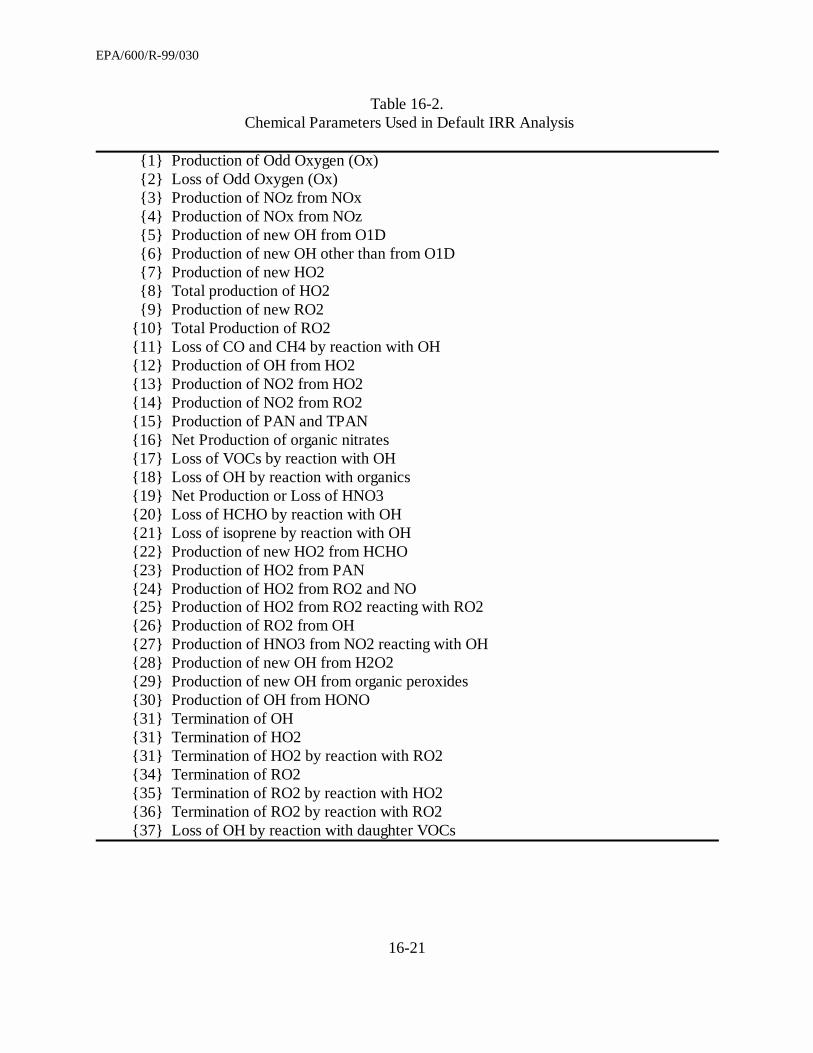
Table 16-2 lists the chemical parameters that are produced in this example IRR analysis for theRADM2 mechanism. Most of these parameters could also be generated for other chemicalmechanisms, although the specific calculations that would have to be performed wouldnecessarily differ because of differences in the mechanisms. The parameters in Table 16-2 arecomputed as simple, linear combinations of the IRRs that are calculated for each chemicalreaction. The domain controls that are specified for the integrated process rate outputs apply toIRR outputs as well. Thus, both the IPR and IRR data will be generated for the same domainand written to output files at the same time intervals. Similarly, the IRR output files are standardModels-3 IO/API gridded files, and can be used with the standard Models-3 visualization tools. In addition, a special visualization tool that can generate “default” cycle diagrams similar toFigure 16-3b is available and is described in Models-3 User Manual (EPA, 1998). Note,however, that the IPR and IRR outputs are written to separate files.
One of the advantages of generating IRR data in the form of chemical parameters is that theoutput file storage requirements can often be minimized. Note that there are fewer IRRparameters in Table 16-2 than there are species in most mechanisms. The major disadvantage tothis approach is that new or different parameters cannot be computed without rerunning a modelsimulation. As a consequence, the CMAQ implementation of IRR analysis also contains theoption to capture the complete set of IRRs rather than chemical parameters when a model is run. With this option, one IRR is generated for each chemical reaction, and these IRRs can then bemanipulated in postprocessing routines to form any particular chemical parameter of interest. Thus, it would be anticipated that the chemical parameters such as those in Table 16-2 would begenerated in fairly routine model applications, whereas IRRs for each reaction would begenerated for exploratory analyses. The form of the outputs is controlled by the PACPcommands that are described next.
16.2.4 Use of the PACP to set up an IRR Analysis
As with IPR analysis, the IRR outputs that are generated by the CCTM are controlled bycommands and special operators that are processed by the PACP. The global commands thatwere described in the IPR section also apply to the IRR output. Thus, family names created withthe DEFINE FAMILY may also be used with several of the IRR commands and operators.
EPA/600/R-99/030
16-13
Before describing how the commands are used to construct an IRR analysis, a brief descriptionof each IRR command and operator is first presented. These are divided into three groups: IRRglobal definitions, IRR operators and IRR output commands. Again, the same syntaxconventions are used, i.e., PACP keywords and symbols are in bold type, user supplied valuesare in normal type, alternative inputs are separated by vertical bars, and completely optionalinputs are enclosed in braces.
IRR Global Definitions:
IRR_TYPE = FULL |PARTIAL |NONE;
The IRR_TYPE command defines the type of IRR analysis. Withthe type set to FULL, IRRs for each reaction will be calculated andwritten to the IRR output file, and all other IRR commands will beignored. IRR_TYPE set to PARTIAL indicates that the IRRcommands following this command are to be processed toproduced user defined IRR outputs. Type set to NONE causes allother IRR commands to be ignored and no IRR output to begenerated. If the command is omitted, type PARTIAL is assumed.
DEFINE CYCLE cyclename = species1;
The DEFINE CYCLE command is used to compute the net of allchemical production and loss of a species involved in more thanone cyclical reaction set. Thus, this quantity is computed bysumming the IRRs for all reactions in which a species is consumed,and then subtracting that sum from the sum of the IRRs for allreactions in which the species is produced. The “cyclename” is auser defined name that must be unique, and can be referenced insubsequent IRR_OUTPUT commands.
The RXSUM command is used to compute a linear combination of IRRs for individual reactions that can then be referenced in asubsequent IRR_OUTPUT command; “sumname” is user definedand must be unique. The linear combination of IRRs is definedaccording to the expressions following the equal signs that specifythe reaction IRRs to sum. The “rxlabli” is the reaction label that isused by the generalized mechanism to identify each reaction and isenclosed in “<” and “>”. The “ci” are optional numericalcoefficients that default to one if not specified.
The production operator (PROD) is used to compute the totalproduction of a species by summing the IRRs of all reactions inwhich species1 appears as a product. The optional qualifiersFROM, AND, and OR restrict the sum to include only thosereactions in which species2 and/or species3 are reactants; “species1"can be any gas-phase mechanism species or a family of gas-phasespecies that was defined using the DEFINE FAMILY command asdescribed in the IPR section; “species2" or species3" may also bethe keyword HV to restrict the selection to photolytic reactions.
The net production operator (NETP) is very similar to theproduction operator PROD since it is used to compute theproduction of a species. Whereas the PROD operator includesevery reaction in which species occurs as a product, the NETPoperator includes only those reactions in which the net productionof species1 is greater than zero. Thus, if species1 appears as both areactant and a product with equal stoichiometry in a reaction, thePROD operator will include it but the NETP operator will not. This operator is useful for getting the net production of a family,for example, by eliminating those reactions in which the net effectof the reaction on the family concentration is zero. The qualifiersFROM, AND and OR restrict the inclusion of reactions to those inwhich species2 and/or species3 are reactants.
LOSS[species1] {AND|OR [species2] }
The loss operator (LOSS) is used to compute the total loss of aspecies by summing the IRRs of all reactions in which species1
appears as a reactant. The optional qualifier AND restricts the sumto include only those reactions in which both species1 and species2
are reactants. Similarly, the OR qualifier includes all reactions inwhich either “species1" or “species2" appears as a reactant. The“species1" or “species2" can be any gas-phase species in themechanism, a family name that includes only gas-phase mechanismspecies, or the keyword HV to restrict the selection of reactions tothose that are photolytic.
NETL[ species1] {AND|OR [species2] }}
EPA/600/R-99/030
16-15
The net loss operator (NETL) is very similar to the loss operatorsince it is used to compute the loss of a species. However, itincludes only those reactions in which there is a net loss of“species1" and/or “species2" . Thus, if species1 appears as both areactant and a product with equal stoichiometry in the reaction, theNETL operator will not include it in summing the loss of thatspecies, whereas the LOSS operator will include the IRR for thatreaction. This operator is useful for getting the net loss of a familyof species.
NET[species1]
The net operator (NET) is very similar to the CYCLE definitionsince it gives the net of the production and the loss of a species forall reactions in which “species1" appears either as reactant or aproduct; “species1" may be any gas-phase, mechanism species orany family consisting wholly of gas-phase mechanism species.
The IRR_OUTPUT command defines a specific IRR output to begenerated during a CCTM simulation. It is constructed byspecifying a linear combination of IRR operators, IRR globaldefinitions, or IRRs for specified reactions. Each individual termin the combination must include either one of the five IRRoperators just described (i.e., opi), a cycle name, a reaction sumname, or a reaction label enclosed in “greater than” and “lessthan” signs. The optional qualifiers (quali) for cyclename orreaction sum name can be either POSONLY or NEGONLY. Withthese qualifiers, the defined quantity is included as a term onlywhen it is positive or negative, respectively. If the name is notqualified, the quantity is included regardless of sign. Thenumerical coefficients for each term (ci) are assumed to be oneunless they are explicitly included. The irrname that is supplied bythe user will be assigned as the variable name in the IO/API IRRoutput file.
DESCRIPTION = ' description';
The description command is provided to allow the user to specify along description of the output variable that will be included on the
EPA/600/R-99/030
16-16
IO/API IRR output name. If a description is not specified for anIRR_OUTPUT variable, the irrname (or short name) will be used inthe output file. If the description command is used, it should belocated immediately following the IRR_OUTPUT command towhich it applies.
Before describing how these commands are actually used, some additional comments arewarranted. First, the specification of any particular IRR output might be accomplished in severaldifferent ways. For example, the net production of a species could be obtained using a CYCLEdefinition, a RXNSUM definition, a NET operator, or simply specifying the appropriate sum ofIRRs directly in the IRR_OUTPUT command (i.e., via reaction labels). Although the user is freeto choose any particular approach, some computational efficiencies may be achieved by usingthe CYCLE and RXNSUM definitions. The CCTM has been constructed to compute thesequantities just once, and then use them whenever they are referenced in an output command. Conversely, operator quantities are recomputed every time they are referenced. Thus, it is moreefficient to use the RXNSUM and CYCLE commands when they can be referenced severaldifferent times in IRR_OUTPUT commands. Second, the NETP and NETL operators areprobably most useful for computing the production and loss of species families. When theseoperators are used, a reaction is not included in the sum if there is no net loss or production of afamily member in the reaction. Thus, all reactions are eliminated from the computations when amember of a family is formed from another member of the same family and there is no netimpact on the family concentration. Finally, the sign conventions employed in the CMAQprocess analysis need to be defined. IRRs for individual chemical reactions are always positive. Since IRRs can be subtracted when computing CYCLE, RXNSUM, and NET quantities, theresult can be either positive or negative. The production and loss operators always producepositive values, however, since individual IRRs are always summed in their computation.
To illustrate how these PACP commands are used to generate IRR output data, two examples arepresented. The first illustrates how to capture IRRs for each reaction. The second demonstrateshow PACP commands are used to compute the special chemical parameters in Table 16-2 for theRADM2 chemical mechanism.
Exhibit 16-3 contains the PACP commands for the first example that corresponds to a full IRRanalysis since IRRs will be calculated for each and every reaction. This option is invoked by thefirst command that specifies that the IRR analysis type is FULL . Since no OUTPUT_DOMAINcommand is present, the IRR outputs will be generated for every cell in the modeling domain.
Exhibit 16-4 shows the PACP commands for the example IRR analysis that has been set up forthe RADM2 chemical mechanism. In a PACP command file, all lines that start with anexclamation point (!) in the first column are comments. To facilitate the discussion below,comment lines have been used to block the IRR commands into special groups. The first fourgroups contain global commands or definitions. All blocks after the first four contain the IRRcommands that generate the particular parameters listed in Table 16-2.
EPA/600/R-99/030
16-17
The commands in the first group simply define the type of IRR analysis and the domain forwhich the IRR outputs are to be generated. The second group includes family definitions. Thesecommands are of the same form as described for IPRs. The remaining two groups of commandsdefine chemical cycles and reaction sums that are subsequently referenced in IRR_OUTPUTcommands. As noted above, the cycle commands give the net production or loss of a species byall chemical reactions. Several of the reaction sums that are defined here are also cycles in thatthey generate the net effect of a few reactions on the production or loss of a few particularspecies. Most of the others are used to define special quantities. For example, the definedRXNSUM newMO2 in Exhibit 16-4 corresponds to the production of new MO2, where newrefers to an initiation reaction for the radical MO2. As is apparent from the IRR_OUTPUTcommands in the subsequent blocks, the cycle and reaction-sum names are referenced fairlyfrequently.
All of the remaining blocks of commands in Exhibit 16-4 contain the commands for IRR outputs. Again, one IRR output is generated for each IRR_OUTPUT command, and the outputs that areproduced correspond to the chemical parameters listed in Table 16-2. As indicated above, eachoutput is generated by the defined linear combination of predefined cycles, reaction sums, specialIRR operators, and/or specified reaction IRRs referenced by reaction label. It should be evidentthat these commands are mechanism specific and require analysis of the mechanism itself toformulate. Thus, this particular PACP command file would not be applicable to any mechanismother than the RADM2. It should also be apparent that other important chemical parameterscould be formulated and generated in an analogous manner. In fact, this command file can beused as the starting point for adding to or modifying some of the selected chemical parameters.
As with IPR outputs, the CCTM will generate the IRR output data in a form comparable to theoutput concentration files. That is, the data are contained in standard Models-3 IO/API griddeddata files. The IRR outputs are linear combinations of individual reaction throughput, and thushave the same units as the gas-phase species concentrations (i.e., ppms). However, it should beremembered that these are throughputs calculated by integrating reaction rates over the outputtime interval, and not simply abundances at a particular time.
16.3 Conclusion
Process Analysis is a diagnostic method for evaluating the inner workings of a model. Althoughspecific types of techniques have been performed and used in the past, new ways of examiningand analyzing process data are likely to be developed and used in the future. As a consequence,the emphasis in the CMAQ implementation of process analysis has been placed on providingeasy methods of extracting key process data from the CCTM simulations. The CMAQimplementation also provides tools to allow users to customize their analyses. These tools aredesigned to be easy to use and not require coding changes to the model.
As noted previously, a process analysis is set up by using the PACP before constructing andrunning a CCTM simulation. Both IPR and IRR data can be gathered during a simulation, buteach are written to separate output files. To collect both sets of output during a single simulation
EPA/600/R-99/030
16-18
requires that the PACP command file contain both the IPR commands and the IRR commands. Although the IPR and IRR examples have been presented separately, both sets of outputs can beproduced with a single file containing both sets of commands. Recall, however, that theOUTPUT_DOMAIN applies to both the IPR outputs and the IRR outputs. Thus, IPR and IRRdata cannot be generated for different parts of the domain in the same simulation.
The PACP program performs a substantial amount of error checking. The program will checkfor the proper syntax of the input commands and perform some logic checking. For example, itchecks to make sure that all species referenced in IRR commands are gas-phase mechanismspecies and that the members of defined families are either all gas-phase species or all aerosolspecies. As is apparent from Exhibit 16-4, however, the inputs for a comprehensive IRR analysiscan be fairly extensive. As a consequence, the PACP produces an output report that summarizeswhat IRR and IPR outputs are being requested. One of its major functions is to report on theeffects of the special IRR operators that are used in the PACP command file. A user may wishto review this report before proceeding to run the CCTM to insure that the desired outputs willbe generated. The reader is referred to the Models-3 User Manual (EPA, 1998) for an exampleoutput report.
Finally, the default configuration for the CCTM is to omit process analysis outputs entirely. Thus,no process analysis will be generated in this configuration. Any process analysis must be set upin the Science Manager of the Models-3 framework. The reader is referred to the Models-3 UserManual (EPA, 1998) for details on how this is done.
16.4 References
Jang, J. C., H. E. Jeffries, D. Byun, and J. E. Pleim, 1995a. “Sensitivity of Ozone to Model GridResolution - I. Application of High-resolution Regional Acid Deposition Model”, AtmosphericEnvironment, Volume 29, No. 21, 3085-3100.
Jang, J. C., H. E. Jeffries, and S. Tonnesen, 1995b. “Sensitivity of Ozone to Model GridResolution - II. Detailed Process Analysis for Ozone Chemistry”, Atmospheric Environment,Volume 29, No. 21, 3101-3114..
Jeffries, H. E., 1995. “Photochemical Air Pollution,” Chapter 9 in Composition, Chemistry, andClimate of the Atmosphere, Ed. H. B. Singh, Van Nostand-Reinhold, New York, N.Y.
Jeffries, H.E., 1996. “Ozone Chemistry and Transport”, presentation to the FACA subcommitteefor Ozone, Particulate Matter and Regional Haze Implementation, March 21, Alexandria, Va.
Jeffries, H. E. and S. Tonnesen, 1994. “A Comparison of Two Photochemical ReactionMechanisms Using Mass Balance and Process Analysis”, Atmospheric Environment, Volume 28,No. 18, 2991-3003.
EPA/600/R-99/030
16-19
Pleim, J.E., 1990. Development and Application of New Modeling Techniques for MesoscaleAtmospheric Chemistry, Ph.D. Thesis, State University of new York at Albany, Albany, NewYork.
Seinfeld, J. H. and S. N. Pandis, 1998. Atmospheric Chemistry and Physics, From Air Pollutionto Climate Change, John Wiley and Sons, New York, New York.
Tonnesen, S. and H. E. Jeffries, 1994. “Inhibition of Odd Oxygen Production in the CarbonBond Four and Generic Reaction Set Mechanisms”, Atmospheric Environment, Volume 28, No.7, 1339-1349.
This chapter is taken from Science Algorithms of the EPA Models-3 CommunityMultiscale Air Quality (CMAQ) Modeling System, edited by D. W. Byun and J. K. S.Ching, 1999.
EPA/600/R-99/030
16-20
Table 16-1. CCTM Processes and PACP Codes
PACP Code Process Description
XADV Adv ection in the E-W directionYADV Adv ection in the N-S directionZADV Vertical advectionADJC Mass adjustment for advectionHDIF Horizontal diffusionVDIF Vertical diffusionEMIS EmissionsDDEP Dry depositionCHEMChemistryAERO AerosolsCLDS Cloud processes and aqueous chemistryPING Plume-in-grid
Note: The following process codes can also be used in the PACP. XYADV Sum of XADV and YADVXYZADV Sum of XADV, YADV, and ZADVTOTADV Sum of XADV, YADV, ZADV, and ADJCTOTDIF Sum of HDIF and VDIFTOTTRAN Sum of XADV, YADV, ZADV, ADJC, HDIF and VDIF
EPA/600/R-99/030
16-21
Table 16-2. Chemical Parameters Used in Default IRR Analysis
{1} Production of Odd Oxygen (Ox) {2} Loss of Odd Oxygen (Ox) {3} Production of NOz from NOx {4} Production of NOx from NOz {5} Production of new OH from O1D {6} Production of new OH other than from O1D {7} Production of new HO2 {8} Total production of HO2 {9} Production of new RO2 {10} Total Production of RO2 {11} Loss of CO and CH4 by reaction with OH {12} Production of OH from HO2 {13} Production of NO2 from HO2 {14} Production of NO2 from RO2 {15} Production of PAN and TPAN {16} Net Production of organic nitrates {17} Loss of VOCs by reaction with OH {18} Loss of OH by reaction with organics {19} Net Production or Loss of HNO3 {20} Loss of HCHO by reaction with OH {21} Loss of isoprene by reaction with OH {22} Production of new HO2 from HCHO {23} Production of HO2 from PAN {24} Production of HO2 from RO2 and NO {25} Production of HO2 from RO2 reacting with RO2 {26} Production of RO2 from OH {27} Production of HNO3 from NO2 reacting with OH {28} Production of new OH from H2O2 {29} Production of new OH from organic peroxides {30} Production of OH from HONO {31} Termination of OH {31} Termination of HO2 {31} Termination of HO2 by reaction with RO2 {34} Termination of RO2 {35} Termination of RO2 by reaction with HO2 {36} Termination of RO2 by reaction with RO2 {37} Loss of OH by reaction with daughter VOCs
EPA/600/R-99/030
16-22
Exhibit 16-1.Example PACP Command File for IPR Analysis
Exhibit 16-3. Example PACP Command File for a Full IRR Analysis
IRR_TYPE = FULL;
ENDPA;
EPA/600/R-99/030
16-27
Exhibit 16-4. Example PACP Commands for a Partial IRR Analysis
!***********************************************************************! Example PACP Command File illustrating Partial IRR Analysis!***********************************************************************
!=======================================================================! IRR type and domain commands !=======================================================================
IRRTYPE = PARTIAL;
OUTPUT_DOMAIN = LOLEV[1] + HILEV[2];
!=======================================================================! Family Definitions !=======================================================================DEFINE FAMILY OX = O3 + NO2 + 2*NO3 + O3P +O1D + PAN + HNO4 + 3*N2O5 + TPAN + OLN + HNO3 + ONIT;DEFINE FAMILY NOZ = PAN + TPAN + HONO + HNO4 + NO3 + N2O5 + ONIT + OLN + HNO3;DEFINE FAMILY NOX = NO + NO2;DEFINE FAMILY VOCA = OL2 + OLI + OLT + ISO;DEFINE FAMILY RO2 = MO2 + ETHP + HC3P + HC5P + HC8P + OL2P + OLTP + OLIP + TOLP + XYLP + ACO3 + KETP + TCO3 + XO2 + XNO2;DEFINE FAMILY VOC = {CH4 +} CO + ETH + HC3 + HC5 + HC8 + OL2 + OLT + OLI + ISO + TOL + CSL + XYL + HCHO + ALD + KET + GLY + MGLY + DCB;DEFINE FAMILY dauHC = CSL + KET + GLY + MGLY + DCB + OP1 + OP2 + PAA + PAN + ONIT;
!=======================================================================! IRR_OUTPUT 5: Production of new OH from O1D!=======================================================================IRR_OUTPUT OHfromO1D = PROD [HO] FROM [O1D];
DESCRIPTION = 'OH produced from O1D';
!=======================================================================! IRR_OUTPUT 6: Production of new OH other than from O1D!=======================================================================IRR_OUTPUT newOH = 0.1*< 85> + 0.14*< 86> + 0.1*< 87> + 2*H2O2_OHcyc[POSONLY] + HNO3_OHcyc[POSONLY] + HONOcyc[NEGONLY] + OP1_OHcyc[POSONLY] + OP2_OHcyc[POSONLY] + PAA_OHcyc[POSONLY];
!=======================================================================! IRR_OUTPUT 8: Total Production of HO2!=======================================================================IRR_OUTPUT totalHO2 = 2.0*<P11> + <P12> + 0.8*<P18> + <P19> + 0.98*<P20> + <P21> + < 74> + < 76> + 0.12*< 84> + {HO2new} 0.23*< 85> + 0.26*< 86> + 0.23*< 87> + OP1_OHcyc[POSONLY] + OP2_HO2cyc[POSONLY] + HNO4_HO2cyc[POSONLY] + {HO2propbyOH} PROD[HO2] FROM [HO] AND [VOC] + {HO2viaRO2_NO} PROD[HO2] FROM [NO] AND [RO2] + {HO2byRO2_RO2} PROD[HO2] FROM [RO2] AND [RO2] + {otherOH} HOXcyc[POSONLY]; DESCRIPTION = 'total HO2';
!=======================================================================! IRR_OUTPUT 9: Production of new RO2!=======================================================================IRR_OUTPUT newRO2 = newMO2 + newACO3 + newETHP + newTCO3 + PAN_ACO3cyc[POSONLY] + TPAN_TCO3cyc[POSONLY];
DESCRIPTION = 'new RO2';
!=======================================================================! IRR_OUTPUT 10: Total Production of RO2!=======================================================================IRR_OUTPUT TotalRO2 = newMO2 + newACO3 + {newRO2} newETHP + newTCO3 + PAN_ACO3cyc[POSONLY] + TPAN_TCO3cyc[POSONLY] + {propRO2_OH} PROD[RO2] FROM [HO] AND [VOC] + < 30> + 0.5*< 47> + 0.5*<48> + < 50> + < 51> + {propRO2_NO} PROD[RO2] FROM [NO];
DESCRIPTION = 'Total RO2';
!=======================================================================! IRR_OUTPUT 11: Loss of CO & CH4 by reaction with OH!=======================================================================IRR_OUTPUT Loss_CO_CH4 = < 30> + LOSS [CO];
DESCRIPTION = 'Loss of CO & CH4';
!=======================================================================! IRR_OUTPUT 12: Production of OH from HO2
EPA/600/R-99/030
Exhibit 16-4. Example PACP Commands for a Partial IRR Analysis
!=======================================================================! IRR_OUTPUT 13: Production of NO2 from HO2!=======================================================================IRR_OUTPUT NO2fromHO2 = < 9>;
!=======================================================================! IRR_OUTPUT 15: Production of PAN and TPAN!=======================================================================IRR_OUTPUT prodPAN_TPAN = PANcyc + TPANcyc;
DESCRIPTION = 'Production of PAN and TPAN';
!=======================================================================! IRR_OUTPUT 16: Net Production of organic nitrates!=======================================================================IRR_OUTPUT netONIT = NET[ONIT];
DESCRIPTION = 'Net production of ONIT';
!=======================================================================! IRR_OUTPUT 17: Loss of VOCs by reaction with OH!=======================================================================IRR_OUTPUT lossOH_HC = LOSS[VOC] AND [HO] + < 30> + < 47> + < 48> + < 49> + < 50> + < 51>;
DESCRIPTION = 'Loss of HC plus OH';
!=======================================================================! IRR_OUTPUT 18: Loss of OH by reaction with inorganics!=======================================================================IRR_OUTPUT lossOH_INORG = < 7> + < 14> + < 15> + < 24> + < 25> + < 26> + < 27>;
DESCRIPTION = 'Loss of OH with iorganics';
!=======================================================================! IRR_OUTPUT 19: Net production or loss of HNO3!=======================================================================IRR_OUTPUT netHNO3 = NET[HNO3];
DESCRIPTION = 'Net change in HNO3';
EPA/600/R-99/030
Exhibit 16-4. Example PACP Commands for a Partial IRR Analysis
16-31
!=======================================================================! IRR_OUTPUT 20: Loss of HCHO by reaction with OH!=======================================================================IRR_OUTPUT lossHCHO_OH = LOSS[HCHO] AND [HO];
DESCRIPTION = 'Reaction OH HCHO with OH';
!=======================================================================! IRR_OUTPUT 21: Loss of isoprene by reaction with OH!=======================================================================IRR_OUTPUT lossISO_OH = LOSS[ISO] AND [HO];
DESCRIPTION = 'Reaction of ISO with OH';
!=======================================================================! IRR_OUTPUT 22: Production of new HO2 from HCHO!=======================================================================IRR_OUTPUT newHO2fromHCHO = PROD[HO2] FROM [HCHO] AND [hv];
DESCRIPTION = 'New HO2 from HCHO';
!=======================================================================! IRR_OUTPUT 23: Production of HO2 from PAN!=======================================================================IRR_OUTPUT HO2fromPAN = PAN_ACO3cyc[POSONLY];
DESCRIPTION = 'HO2 from PAN';
!=======================================================================! IRR_OUTPUT 24: Production of HO2 from RO2 and NO!=======================================================================IRR_OUTPUT HO2fromRO2_NO = PROD[HO2] FROM [NO] AND [RO2];
DESCRIPTION = 'HO2 from RO2 and NO';
!=======================================================================! IRR_OUTPUT 25: Production of HO2 from RO2 and RO2!=======================================================================IRR_OUTPUT HO2fromRO2_RO2 = PROD[HO2] FROM [RO2] AND [RO2];
DESCRIPTION = 'HO2 from RO2 and RO2';
!=======================================================================! IRR_OUTPUT 26: Production of RO2 from OH!=======================================================================IRR_OUTPUT RO2fromOH = PROD[RO2] FROM [HO];
DESCRIPTION = 'RO2 from OH';
!=======================================================================! IRR_OUTPUT 27: Production of HNO3 from OH + NO2!=======================================================================IRR_OUTPUT HNO3fromOH_NO2 = < 24>;
DESCRIPTION = 'HNO3 from OH + NO2';
!=======================================================================! IRR_OUTPUT 28: Production of new OH from H2O2!=======================================================================IRR_OUTPUT newOH_H2O2 = 2*H2O2_OHcyc[POSONLY];
DESCRIPTION = 'new OH from H2O2';
EPA/600/R-99/030
Exhibit 16-4. Example PACP Commands for a Partial IRR Analysis
16-32
!=======================================================================! IRR_OUTPUT 29: Production of new OH from organic peroxides!=======================================================================IRR_OUTPUT newOH_OP1 = OP1_OHcyc[POSONLY] + OP2_OHcyc[POSONLY] + PAA_OHcyc[POSONLY];
DESCRIPTION = 'new OH from OP1 OP2 PAA';
!=======================================================================! IRR_OUTPUT 30: Production of OH from HONO!=======================================================================IRR_OUTPUT newOHfromHONO = HONOcyc[NEGONLY];
!=======================================================================! IRR_OUTPUT 35: Termination of RO2 by reaction with with HO2!=======================================================================IRR_OUTPUT termRO2_HO2 = OP1_OHcyc[NEGONLY] + OP2_OHcyc[NEGONLY] + PAA_OHcyc[NEGONLY];
DESCRIPTION = 'RO2 Termination with HO2';
EPA/600/R-99/030
Exhibit 16-4. Example PACP Commands for a Partial IRR Analysis
!=======================================================================! IRR_OUTPUTs 37: Loss of OH by reaction with daughter VOCs!=======================================================================IRR_OUTPUT dauHC_OH = LOSS [HO] AND [dauHC];
DESCRIPTION = 'OH + daughter HC';
ENDPA;
EPA/600/R-99/030
16-34
Figure 16-1. Example process analyses showing contributions of individual processes to modelpredicted concentrations (Source: Jeffries, 1996).
EPA/600/R-99/030
16-35
Figure 16-2. Example Process Analyses showing model predicted concentrations and processcontributions for different model configurations (Source: Jeffries, 1996).
EPA/600/R-99/030
16-36
Figure 16-3a. Schematic of OH reaction with NO oxidation cycles (Source: Jeffries, 1996).
Figure 16-3b. Example photochemical cycle throughputs derived from integrated reaction rates(Source: Jeffries, 1995).