CHAPTER 2CHAPTER 2 DDIRECT IRECT MMETHODS FOR ETHODS FOR

SSTOCHASTIC TOCHASTIC SSEARCHEARCH

•Organization of chapter in ISSO–Introductory material

–Random search methods•Attributes of random search•Blind random search (algorithm A)•Two localized random search methods (algorithms B and C)

–Random search with noisy measurements

–Nonlinear simplex (Nelder-Mead) algorithm•Noise-free and noisy measurements

Slides for Introduction to Stochastic Search and Optimization (ISSO) by J. C. Spall

2-2

Some Attributes of Direct Random Search Some Attributes of Direct Random Search with Noise-Free Loss Measurementswith Noise-Free Loss Measurements

• Ease of programming

• Use of only L values (vs. gradient values) – Avoid “artful contrivance” of more complex methods

• Reasonable computational efficiency

• Generality – Algorithms apply to virtually any function

• Theoretical foundation – Performance guarantees, sometimes in finite samples

– Global convergence in some cases

2-3

Algorithm A: Algorithm A: Simple Random (“Blind”) SearchSimple Random (“Blind”) Search

Step 0 (initialization) Step 0 (initialization) Choose an initial value of = inside of . Set k = 0.

Step 1 (candidate value)Step 1 (candidate value) Generate a new

independent value new(k+1) , according to the

chosen probability distribution. If L(new(k+1)) <

set = new(k+1). Else take = .

Step 2 (return or stop) Step 2 (return or stop) Stop if maximum number of L evaluations has been reached or user is otherwise satisfied with the current estimate for ; else, return to step 1 with the new k set to the former k+1.

0

( ),kL

1ˆ

k 1ˆ

k k

2-4

First Several Iterations of Algorithm A First Several Iterations of Algorithm A on Problem with Solution on Problem with Solution = [1.0, 1.0] = [1.0, 1.0]T T

(Example 2.1 in (Example 2.1 in ISSOISSO))

Iteration k new(k)T

L(new(k)) Tk ˆ( )kL

0 [2.00, 2.00] 8.00

1 [2.25, 1.62] 7.69 [2.25, 1.62] 7.69

2 [2.81, 2.58] 14.55 [2.25, 1.62] 7.69

3 [1.93, 1.19] 5.14 [1.93, 1.19] 5.14

4 [2.60, 1.92] 10.45 [1.93, 1.19] 5.14

5 [2.23, 2.58] 11.63 [1.93, 1.19] 5.14

6 [1.34, 1.76] 4.89 [1.34, 1.76] 4.89

2-5

(a) Continuous L(); probability density for new is > 0 on = [0, )

(b) Discrete L(); discrete sampling for new with

P(new = i ) > 0 for i = 0, 1, 2,...

(c) Noncontinuous L(); probability density for new

is > 0 on = [0, )

Functions for Convergence (Parts (a) Functions for Convergence (Parts (a) and(b)) and Nonconvergence (Part (c)) of and(b)) and Nonconvergence (Part (c)) of

Blind Random SearchBlind Random Search

2-6

Algorithm B: Algorithm B: Localized Random SearchLocalized Random Search

Step 0 (initialization) Step 0 (initialization) Choose an initial value of = inside of . Set k = 0.

Step 1 (candidate value)Step 1 (candidate value) Generate a random dk. Check if

. If not, generate new dk or move to nearest valid

point. Let new(k+1) be or the modified point.

Step 2 (check for improvement) Step 2 (check for improvement) If L(new(k+1)) < set

= new(k+1). Else take = .

Step 3 (return or stop) Step 3 (return or stop) Stop if maximum number of L evaluations has been reached or if user satisfied with current estimate; else, return to step 1 with new k set to former k+1.

0

( ),kL

1ˆ

k

k kd k kdk kd

1ˆ

k k

2-7

Algorithm C: Algorithm C: Enhanced Localized Random SearchEnhanced Localized Random Search

• Similar to algorithm B

• Exploits knowledge of good/bad directions

• If move in one direction produces decreasedecrease in loss, add bias to next iteration to continuecontinue algorithm moving in “good” direction

• If move in one direction produces increaseincrease in loss, add bias to next iteration to move algorithm in oppositeopposite way

• Slightly more complex implementation than algorithm B

2-8

Formal Convergence of Random Formal Convergence of Random Search AlgorithmsSearch Algorithms

• Well-known results on convergence of random search

– Applies to convergence of and/or L values

– Applies when noise-freenoise-free L measurements used in algorithms

• Algorithm A (blind random search) converges under very general conditions

– Applies to continuous or discrete functions

• Conditions for convergence of algorithms B and C somewhat more restrictive, but still quite general

– ISSO presents theorem for continuous functions

– Other convergence results exist

• Convergence raterate theory also exists: how fast to converge?

– Algorithm A generally slow in high-dimensional problems

2-9

Example Comparison of Algorithms Example Comparison of Algorithms A, B, and C A, B, and C

• Relatively simple p = 2 problem (Examples 2.3 and 2.4 in ISSO)

– Quartic loss function (plot on next slide)

• One global solution; several local minima/maxima

• Started all algorithms at common initial condition and compared based on common number of loss evaluations

– Algorithm A needed no tuning

– Algorithms B and C required “trial runs” to tune algorithm coefficients

2-10

Multimodal Quartic Loss Function for Multimodal Quartic Loss Function for pp = 2 Problem (Example 2.3 in = 2 Problem (Example 2.3 in ISSOISSO))

2-11

Example 2.3 in Example 2.3 in ISSO ISSO (cont’d): (cont’d): Sample Means of Terminal Values Sample Means of Terminal Values

– – LL(()) in Multimodal Loss Functionin Multimodal Loss Function

(with Approximate 95% Confidence Intervals)(with Approximate 95% Confidence Intervals)

Algorithm A

Algorithm B Algorithm C

2.51 [1.94, 3.08]

0.78 [ 0.51, 1.04]

0.49 [ 0.32, 0.67]

Notes:

Sample means from 40 independent runs.

Confidence intervals for algorithms B and C overlap slightly since 0.51 < 0.67

ˆ( )kL

2-12

Examples 2.3 and 2.4 in Examples 2.3 and 2.4 in ISSO ISSO (cont’d):(cont’d):Typical Adjusted Loss Values ( Typical Adjusted Loss Values ( – – LL(())) )

and and Estimates in Multimodal Estimates in Multimodal Loss Function (One Run)Loss Function (One Run)

Algorithm A

Algorithm B

Algorithm C

Adjusted L value 2.60

0.80

0.49

estimate for above L value

093

552

.

.

902

682

.

.

962

742

.

.

Note: = [2.904, 2.904]T

( )kL

2-13

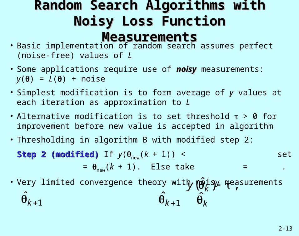
Random Search Algorithms with Noisy Random Search Algorithms with Noisy Loss Function MeasurementsLoss Function Measurements

• Basic implementation of random search assumes perfect (noise-free) values of L

• Some applications require use of noisynoisy measurements: y() = L() + noise

• Simplest modification is to form average of y values at each iteration as approximation to L

• Alternative modification is to set threshold > 0 for improvement before new value is accepted in algorithm

• Thresholding in algorithm B with modified step 2:

Step 2 (modified) Step 2 (modified) If y(new(k+1)) < set =

new(k+1). Else take = .

• Very limited convergence theory with noisy measurements ˆ( ) ,ky

1ˆ

k 1ˆ

kˆ

k

2-14

Nonlinear Simplex (Nelder-Mead) AlgorithmNonlinear Simplex (Nelder-Mead) Algorithm

• Nonlinear simplex method is popular search method (e.g., fminsearch in MATLAB)

• Simplex is convex hull of p + 1 points in p

– Convex hull is smallest convex set enclosing the p + 1 points

– For p = 2 convex hull is triangle

– For p = 3 convex hull is pyramid

• Algorithm searches for by moving convex hull within • If algorithm works properly, convex hull shrinks/collapses

onto

• No injected randomness (contrast with algorithms A, B, and C), but allowance for noisy loss measurements

• Frequently effective, but no general convergence theory and many numerical counterexamples to convergence

2-15

Steps of Nonlinear Simplex AlgorithmSteps of Nonlinear Simplex Algorithm

Step 0 (Initialization)Step 0 (Initialization) Generate initial set of p + 1 extreme points in p, i (i = 1, 2, …, p + 1), vertices of initial simplex

Step 1 (Reflection)Step 1 (Reflection) Identify where max, second highest, and min loss values occur; denote them by max, 2max, and min,

respectively. Let cent = centroid (mean) of all i except for max.

Generate candidate vertex refl by reflecting max through cent

using refl = (1 + )cent max ( > 0).

Step 2a (Accept reflection) Step 2a (Accept reflection) If L(min) L(refl) < L(2max), then

refl replaces max; proceed to step 3; else go to step 2b.

Step 2b (Expansion) Step 2b (Expansion) If L(refl) < L(min), then expand reflection

using exp = refl + (1 )cent, > 1; else go to step 2c. If

L(exp) < L(refl), then exp replaces max; otherwise reject

expansion and replace max by refl. Go to step 3.

2-16

Steps of Nonlinear Simplex Algorithm (cont’d)Steps of Nonlinear Simplex Algorithm (cont’d)

Step 2c (Contraction) Step 2c (Contraction) If L(refl) L(2max), then contract

simplex: Either case (i) L(refl) < L(max), or case (ii) L(max)

L(refl). Contraction point is cont = max/refl + (1 )cent, 0

1, where max/refl = refl if case (i), otherwise max/refl = max. In

case (i), accept contraction if L(cont) L(refl); in case (ii),

accept contraction if L(cont) < L(max). If accepted, replace max

by cont and go to step 3; otherwise go to step 2d.

Step 2d (Shrink) Step 2d (Shrink) If L(cont) L(max), shrink entire simplex

using a factor 0 < < 1, retaining only min. Go to step 3.

Step 3 (Termination)Step 3 (Termination) Stop if convergence criterion or maximum number of function evaluations is met; else return to step 1.

2-17

Illustration of Steps of Nonlinear Simplex Illustration of Steps of Nonlinear Simplex Algorithm with Algorithm with pp = 2 = 2

max min

cent

2max refl

Reflection

exp

Expansion whenL(refl) < L(min)

max min

cent

refl

cont

max min

refl

cont

cent

2max

Contraction whenL(refl) L(max)

(“inside”)

Shrink after failed contraction when L(refl) < L(max)

cont

max min

cent

refl

Contraction whenL(refl) < L(max)

(“outside”)

2max 2max

max min

cent

2maxrefl