CHAPTER 2 GENERIC METHODOLOGIES APPLICABLE TO MULTIPLE ... · Chapter 2: Generic Methodologies...

Chapter 2: Generic Methodologies Applicable to Multiple Land-Use Categories

2006 IPCC Guidelines for National Greenhouse Gas Inventories 2.1

C H A P T E R 2

GENERIC METHODOLOGIES APPLICABLE TO MULTIPLE LAND-USE CATEGORIES

Volume 4: Agriculture, Forestry and Other Land Use

2.2 2006 IPCC Guidelines for National Greenhouse Gas Inventories

Authors Harald Aalde (Norway), Patrick Gonzalez (USA), Michael Gytarsky (Russian Federation), Thelma Krug (Brazil), Werner A. Kurz (Canada), Rodel D. Lasco (Philippines), Daniel L. Martino (Uruguay), Brian G. McConkey (Canada), Stephen Ogle (USA), Keith Paustian (USA), John Raison (Australia), N.H. Ravindranath (India), Dieter Schoene (FAO), Pete Smith (UK), Zoltan Somogyi (European Commission/Hungary), Andre van Amstel (Netherlands), and Louis Verchot (ICRAF/USA)



Contents

2 Generic Methodologies Applicable to Multiple Land-use Categories 2.1 Introduction ...........................................................................................................................................2.6 2.2 Inventory framework.............................................................................................................................2.6

2.2.1 Overview of carbon stock change estimation................................................................................2.6 2.2.2 Overview of non-CO2 emission estimation .................................................................................2.10 2.2.3 Conversion of C stock changes to CO2 emissions.......................................................................2.11

2.3 Generic methods for CO2 emissions and removals .............................................................................2.11 2.3.1 Change in biomass carbon stocks (above-ground biomass and below-ground biomass) ............2.11

2.3.1.1 Land remaining in a land-use category ..................................................................................2.12 2.3.1.2 Land converted to a new land-use category...........................................................................2.19

2.3.2 Change in carbon stocks in dead organic matter .........................................................................2.21 2.3.2.1 Land remaining in a land-use category ..................................................................................2.21 2.3.2.2 Land conversion to a new land-use category .........................................................................2.25

2.3.3 Change in carbon stocks in soils .................................................................................................2.28 2.3.3.1 Soil C estimation methods (land remaining in a land-use category and

land conversion to a new land use) ........................................................................................2.29 2.4 Non-CO2 emissions .............................................................................................................................2.40 2.5 Additional generic guidance for Tier 3 methods .................................................................................2.50

2.5.1 Measurement-based Tier 3 inventories........................................................................................2.50 2.5.2 Model-based Tier 3 inventories...................................................................................................2.52

References .....................................................................................................................................................2.54

Equations

Equation 2.1 Annual carbon stock changes for the entire AFOLU Sector estimated as the sum of changes in all land-use categories..............................................................................2.6

Equation 2.2 Annual carbon stock changes for a land-use category as a sum of changes in each stratum within the category .......................................................................................2.7

Equation 2.3 Annual carbon stock changes for a stratum of a land-use category as a sum of changes in all pools ...........................................................................................................2.7

Equation 2.4 Annual carbon stock change in a given pool as a function of gains and losses (Gain-Loss Method)....................................................................................................2.9

Equation 2.5 Carbon stock change in a given pool as an annual average difference between estimates at two points in time (Stock-Difference Method) ..................................2.10

Equation 2.6 Non-CO2 emissions to the atmosphere ................................................................................2.10

Equation 2.7 Annual change in carbon stocks in biomass in land remaining in a particular land-use category (Gain-Loss Method) ...............................................................2.12



Equation 2.8 Annual change in carbon stocks in biomass in land remaining in the same land-use category (Stock-Difference Method) ...........................................................2.12

Equation 2.9 Annual increase in biomass carbon stocks due to biomass increment in land remaining in same category .....................................................................................2.15

Equation 2.10 Average annual increment in biomass .................................................................................2.15

Equation 2.11 Annual decrease in carbon stocks due to biomass losses in land remaining in same category ..................................................................................................................2.16

Equation 2.12 Annual carbon loss in biomass of wood removals...............................................................2.17

Equation 2.13 Annual carbon loss in biomass of fuelwood removal..........................................................2.17

Equation 2.14 Annual carbon losses in biomass due to disturbances .........................................................2.18

Equation 2.15 Annual change in biomass carbon stocks on land converted to other land-use category (Tier 2)....................................................................................................2.20

Equation 2.16 Initial change in biomass carbon stocks on land converted to another land category..........2.20

Equation 2.17 Annual change in carbon stocks in dead organic matter......................................................2.21

Equation 2.18 Annual change in carbon stocks in dead wood or litter (Gain-Loss Method)......................2.23

Equation 2.19 Annual change in carbon stocks in dead wood or litter (Stock-Difference Method)...........2.23

Equation 2.20 Annual carbon in biomass transferred to dead organic matter.............................................2.24

Equation 2.21 Annual biomass carbon loss due to mortality ......................................................................2.24

Equation 2.22 Annual carbon transfer to slash ...........................................................................................2.25

Equation 2.23 Annual change in carbon stocks in dead wood and litter due to land conversion................2.26

Equation 2.24 Annual change in carbon stocks in soils..............................................................................2.29

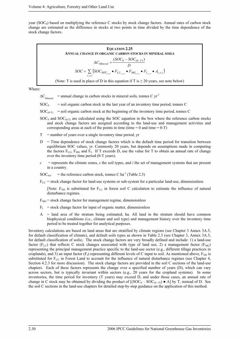
Equation 2.25 Annual change in organic carbon stocks in mineral soils....................................................2.30

Equation 2.26 Annual Carbon loss from drained organic soils (CO2) ........................................................2.35

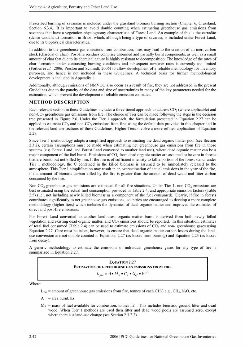
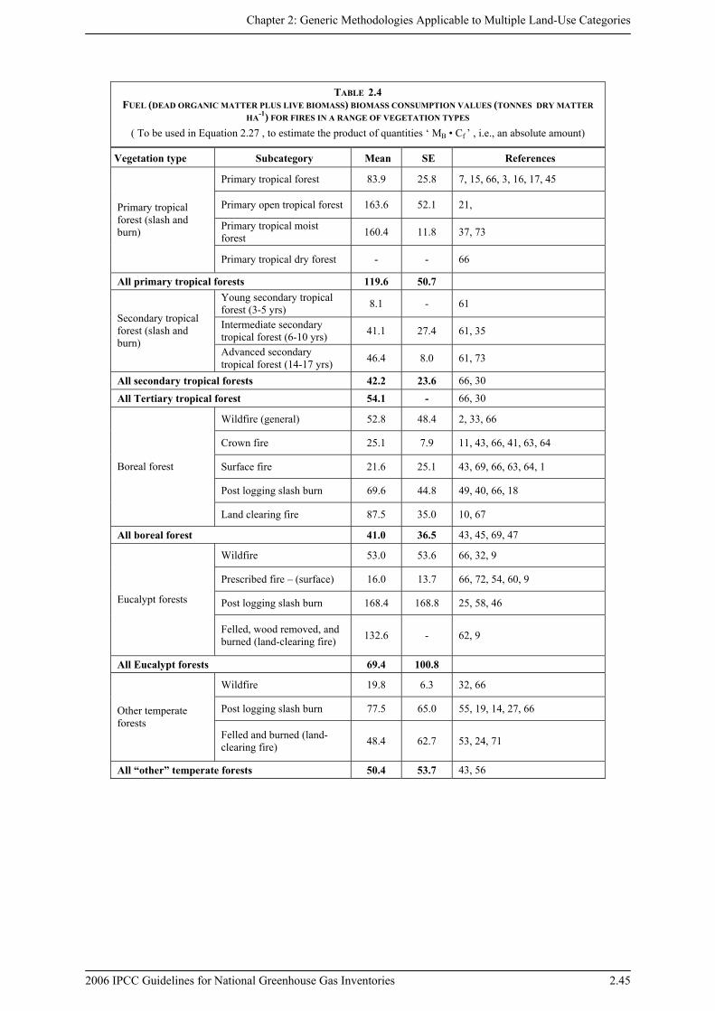
Equation 2.27 Estimation of greenhouse gas emissions from fire ..............................................................2.42

Figures

Figure 2.1 Generalized carbon cycle of terrestrial AFOLU ecosystems showing the flows of carbon into and out of the system as well as between the five C pools within the system.........................................................................................2.8

Figure 2.2 Generic decision tree for identification of appropriate tier to estimate changes in carbon stocks in biomass in a land-use category. ..............................................2.14

Figure 2.3 Generic decision tree for identification of appropriate tier to estimate changes in carbon stocks in dead organic matter for a land-use category ...........................2.22

Figure 2.4 Generic decision tree for identification of appropriate tier to estimate changes in carbon stocks in mineral soils by land-use category..........................................2.32

Figure 2.5 Generic decision tree for identification of appropriate tier to estimate changes in carbon stocks in organic soils by land-use category ..........................................2.33

Figure 2.6 Generic decision tree for identification of appropriate tier to estimate greenhouse gas emissions from fire in a land-use category....................................................................2.44

Figure 2.7 Steps to develop a Tier 3 model-based inventory estimation system. .................................2.52



Tables

Table 2.1 Example of a simple matrix (Tier 2) for the impacts of disturbances on carbon pools .......2.19 Table 2.2 Tier 1 default values for litter and dead wood carbon stocks ..............................................2.27 Table 2.3 Default reference (under native vegetation) soil organic C stocks (SOCREF) for

Mineral Soils .......................................................................................................................2.31 Table 2.4 Fuel (dead organic matter plus live biomass) biomass consumption values

for fires in a range of vegetation types ................................................................................2.45 Table 2.5 Emission factors for various types of burning .....................................................................2.47 Table 2.6 Combustion factor values (proportion of prefire fuel biomass consumed) for fires

in a range of vegetation types ..............................................................................................2.48

Boxes

Box 2.1 Alternative formulations of Equation 2.25 for Approach 1 activity data versus Approach 2 or 3 activity data with transition matrices.............................................2.34

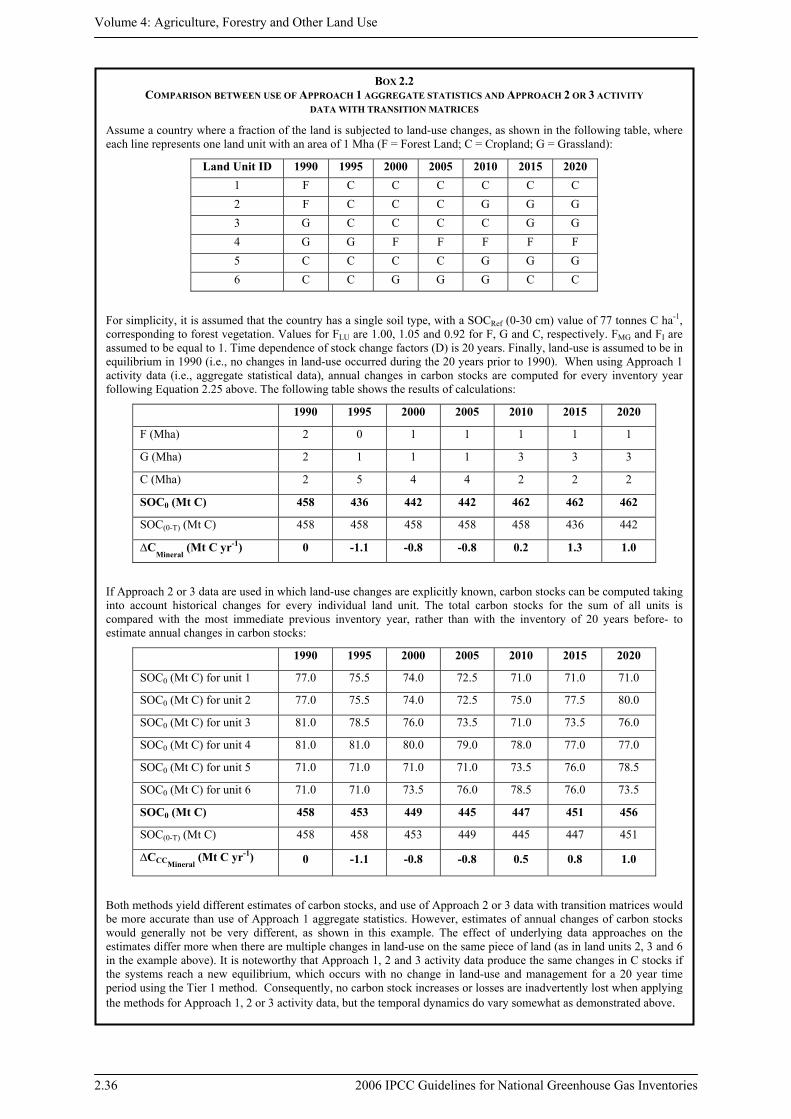
Box 2.2 Comparison between use of Approach 1 aggregate statistics and Approach 2 or 3 activity data with transition matrices ...........................................................................2.36



2 GENERIC METHODOLOGIES APPLICABLE TO MULTIPLE LAND-USE CATEGORIES

2.1 INTRODUCTION Methods to estimate greenhouse gas emissions and removals in the Agriculture, Forestry and Other Land Use (AFOLU) Sector can be divided into two broad categories: 1) methods that can be applied in a similar way for any of the types of land use (i.e., generic methods for Forest Land, Cropland, Grassland, Wetlands, Settlements and Other Land); and 2) methods that only apply to a single land use or that are applied to aggregate data on a national-level, without specifying land use. Chapter 2 provides mainly descriptions of generic methodologies under category (1) for estimating ecosystem carbon stock changes as well as for estimating non-CO2 fluxes from fire. These methods can be applied for any of the six land-use categories. Generic information on methods includes:

• general framework for applying the methods within specific land-use categories;

• choice of methods, including equations and default values for Tier 1 methods for estimating C stock changes and non-CO2 emissions;

• general guidance on use of higher Tier methods;

• use of the IPCC Emission Factor Data Base (EFDB); and

• uncertainty estimation.

Specific details and guidance on implementing the methods for each of the land-use and land-use conversion categories, including choosing emission factors, compiling activity data and assessing uncertainty, are given in the chapters on specific land-use categories (see Chapters 4 to 9). Guidance on inventory calculations for each specific land use refers back to this chapter for description of methods where they are generic.

2.2 INVENTORY FRAMEWORK This section outlines a systematic approach for estimating carbon stock changes (and associated emissions and removals of CO2) from biomass, dead organic matter, and soils, as well as for estimating non-CO2 greenhouse gas emissions from fire. General equations representing the level of land-use categories and strata are followed by a short description of processes with more detailed equations for carbon stock changes in specific pools by land-use category. Principles for estimating non-CO2 emissions and common equations are then given. Specific, operational equations to estimate emissions and removals by processes within a pool and by category, which directly correspond to worksheet calculations, are provided in Sections 2.3 and 2.4.

2.2.1 Overview of carbon stock change estimation The emissions and removals of CO2 for the AFOLU Sector, based on changes in ecosystem C stocks, are estimated for each land-use category (including both land remaining in a land-use category as well as land converted to another land use). Carbon stock changes are summarized by Equation 2.1.

EQUATION 2.1 ANNUAL CARBON STOCK CHANGES FOR THE ENTIRE AFOLU SECTOR ESTIMATED AS THE SUM

OF CHANGES IN ALL LAND-USE CATEGORIES

OLSLWLGLCLFLAFOLU CCCCCCC Δ+Δ+Δ+Δ+Δ+Δ=Δ

Where:

ΔC = carbon stock change

Indices denote the following land-use categories:

AFOLU = Agriculture, Forestry and Other Land Use

FL = Forest Land



CL = Cropland

GL = Grassland

WL = Wetlands

SL = Settlements

OL = Other Land

For each land-use category, carbon stock changes are estimated for all strata or subdivisions of land area (e.g., climate zone, ecotype, soil type, management regime etc., see Chapter 3) chosen for a land-use category (Equation 2.2). Carbon stock changes within a stratum are estimated by considering carbon cycle processes between the five carbon pools, as defined in Table 1.1 in Chapter 1. The generalized flowchart of the carbon cycle (Figure 2.1) shows all five pools and associated fluxes including inputs to and outputs from the system, as well as all possible transfers between the pools. Overall, carbon stock changes within a stratum are estimated by adding up changes in all pools as in Equation 2.3. Further, carbon stock changes in soil may be disaggregated as to changes in C stocks in mineral soils and emissions from organic soils. Harvested wood products (HWP) are also included as an additional pool.

EQUATION 2.2 ANNUAL CARBON STOCK CHANGES FOR A LAND-USE CATEGORY AS A SUM OF CHANGES IN EACH

STRATUM WITHIN THE CATEGORY ∑Δ=Δi

LULU ICC

Where:

ΔCLU = carbon stock changes for a land-use (LU) category as defined in Equation 2.1.

i = denotes a specific stratum or subdivision within the land-use category (by any combination of species, climatic zone, ecotype, management regime etc., see Chapter 3), i = 1 to n.

EQUATION 2.3 ANNUAL CARBON STOCK CHANGES FOR A STRATUM OF A LAND-USE CATEGORY AS A SUM OF

CHANGES IN ALL POOLS

HWPSOLIDWBBABLU CCCCCCCi

Δ+Δ+Δ+Δ+Δ+Δ=Δ

Where:

ΔCLUi = carbon stock changes for a stratum of a land-use category

Subscripts denote the following carbon pools:

AB = above-ground biomass

BB = below-ground biomass

DW = deadwood

LI = litter

SO = soils

HWP = harvested wood products

Estimating changes in carbon pools and fluxes depends on data and model availability, as well as resources and capacity to collect and analyze additional information (See Chapter 1, Section 1.3.3 on key category analysis). Table 1.1 in Chapter 1 outlines which pools are relevant for each land-use category for Tier 1 methods, including cross references to reporting tables. Depending on country circumstances and which tiers are chosen, stock changes may not be estimated for all pools shown in Equation 2.3. Because of limitations to deriving default data sets to support estimation of some stock changes, Tier 1 methods include several simplifying assumptions:



Figure 2.1 Generalized carbon cycle of terrestrial AFOLU ecosystems showing the flows of carbon into and out of the system as well as between the five C pools within the system.

Litter

Dead wood

Above-groundbiomass

Below-groundbiomass

Soil organicmatter

Harvestedwood products

Increase of carbonstocks due to growth

Carbon fluxes due todiscrete events, i.e., from harvest residues and natural disturbance

Carbon fluxes dueto continuous processes, i.e.decomposition

Transfer of carbonbetween pools



• change in below-ground biomass C stocks are assumed to be zero under Tier 1 (under Tier 2, country-specific data on ratios of below-ground to above-ground biomass can be used to estimate below-ground stock changes);

• under Tier 1, dead wood and litter pools are often lumped together as ‘dead organic matter’ (see discussion below); and

• dead organic matter stocks are assumed to be zero for non-forest land-use categories under Tier 1. For Forest Land converted to another land use, default values for estimating dead organic matter carbon stocks are provided in Tier 1.

The carbon cycle includes changes in carbon stocks due to both continuous processes (i.e., growth, decay) and discrete events (i.e., disturbances like harvest, fire, insect outbreaks, land-use change and other events). Continuous processes can affect carbon stocks in all areas in each year, while discrete events (i.e., disturbances) cause emissions and redistribute ecosystem carbon in specific areas (i.e., where the disturbance occurs) and in the year of the event.

Disturbances may also have long-lasting effects, such as decay of wind-blown or burnt trees. For practicality, Tier 1 methods assume that all post-disturbance emissions (less removal of harvested wood products) are estimated as part of the disturbance event, i.e., in the year of the disturbance. For example, rather than estimating the decay of dead organic matter left after a disturbance over a period of several years, all post-disturbance emissions are estimated in the year of the event.

Under Tier 1, it is assumed that the average transfer rate into dead organic matter (dead wood and litter) is equal to the average transfer rate out of dead organic matter, so that the net stock change is zero. This assumption means that dead organic matter (dead wood and litter) carbon stocks need not be quantified under Tier 1 for land areas that remain in a land-use category1. The rationale for this approach is that dead organic matter stocks, particularly dead wood, are highly variable and site-specific, depending on forest type and age, disturbance history and management. In addition, data on coarse woody debris decomposition rates are scarce and thus it was deemed that globally applicable default factors and uncertainty estimates can not be developed. Countries experiencing significant changes in forest types or disturbance or management regimes in their forests are encouraged to develop domestic data to estimate the impact from these changes using Tier 2 or 3 methodologies and to report the resulting carbon stock changes and non-CO2 emissions and removals.

All estimates of changes in carbon stocks, i.e., growth, internal transfers and emissions, are in units of carbon to make all calculations consistent. Data on biomass stocks, increments, harvests, etc. can initially be in units of dry matter that need to be converted to tonnes of carbon for all subsequent calculations. There are two fundamentally different and equally valid approaches to estimating stock changes: 1) the process-based approach, which estimates the net balance of additions to and removals from a carbon stock; and 2) the stock-based approach, which estimates the difference in carbon stocks at two points in time.

Annual carbon stock changes in any pool can be estimated using the process-based approach in Equation 2.4 which sets out the Gain-Loss Method that can be applied to all carbon gains or losses. Gains can be attributed to growth (increase of biomass) and to transfer of carbon from another pool (e.g., transfer of carbon from the live biomass carbon pool to the dead organic matter pool due to harvest or natural disturbances). Gains are always marked with a positive (+) sign. Losses can be attributed to transfers of carbon from one pool to another (e.g., the carbon in the slash during a harvesting operation is a loss from the above-ground biomass pool), or emissions due to decay, harvest, burning, etc. Losses are always marked with a negative (-) sign.

EQUATION 2.4 ANNUAL CARBON STOCK CHANGE IN A GIVEN POOL AS A FUNCTION OF GAINS AND LOSSES

(GAIN-LOSS METHOD)

LG CCC Δ−Δ=Δ

Where:

ΔC = annual carbon stock change in the pool, tonnes C yr-1

ΔCG = annual gain of carbon, tonnes C yr-1

1 Emissions from litter C stocks are accounted for under Tier 1 for forest conversion to other land-use.



ΔCL = annual loss of carbon, tonnes C yr-1

Note that CO2 removals are transfers from the atmosphere to a pool, whereas CO2 emissions are transfers from a pool to the atmosphere. Not all transfers involve emissions or removals, since any transfer from one pool to another is a loss from the donor pool, but is a gain of equal amount to the receiving pool. For example, a transfer from the above-ground biomass pool to the dead wood pool is a loss from the above-ground biomass pool and a gain of equal size for the dead wood pool, which does not necessarily result in immediate CO2 emission to the atmosphere (depending on the Tier used).

The method used in Equation 2.4 is called the Gain-Loss Method, because it includes all processes that bring about changes in a pool. An alternative stock-based approach is termed the Stock-Difference Method, which can be used where carbon stocks in relevant pools are measured at two points in time to assess carbon stock changes, as represented in Equation 2.5.

EQUATION 2.5 CARBON STOCK CHANGE IN A GIVEN POOL AS AN ANNUAL AVERAGE DIFFERENCE BETWEEN

ESTIMATES AT TWO POINTS IN TIME (STOCK-DIFFERENCE METHOD)

)()(

12

12

ttCC

C tt

−

−=Δ

Where:

ΔC = annual carbon stock change in the pool, tonnes C yr-1

Ct1 = carbon stock in the pool at time t1, tonnes C

Ct2 = carbon stock in the pool at time t2, tonnes C

If the C stock changes are estimated on a per hectare basis, then the value is multiplied by the total area within each stratum to obtain the total stock change estimate for the pool. In some cases, the activity data may be in the form of country totals (e.g., harvested wood) in which case the stock change estimates for that pool are estimated directly from the activity data after applying appropriate factors to convert to units of C mass. When using the Stock-Difference Method for a specific land-use category, it is important to ensure that the area of land in that category at times t1 and t2 is identical, to avoid confounding stock change estimates with area changes.

The process method lends itself to modelling approaches using coefficients derived from empirical research data. These will smooth out inter-annual variability to a greater extent than the stock change method which relies on the difference of stock estimates at two points in time. Both methods are valid so long as they are capable of representing actual disturbances as well as continuously varying trends, and can be verified by comparison with actual measurements.

2.2.2 Overview of non-CO2 emission estimation Non-CO2 emissions are derived from a variety of sources, including emissions from soils, livestock and manure, and from combustion of biomass, dead wood and litter. In contrast to the way CO2 emissions are estimated from biomass stock changes, the estimate of non-CO2 greenhouse gases usually involves an emission rate from a source directly to the atmosphere. The rate (Equation 2.6) is generally determined by an emission factor for a specific gas (e.g., CH4, N2O) and source category and an area (e.g., for soil or area burnt), population (e.g., for livestock) or mass (e.g., for biomass or manure) that defines the emission source.

EQUATION 2.6 NON-CO2 EMISSIONS TO THE ATMOSPHERE

EFAEmission •=

Where:

Emission = non-CO2 emissions, tonnes of the non-CO2 gas

A = activity data relating to the emission source (can be area, animal numbers or mass unit, depending on the source type)

EF = emission factor for a specific gas and source category, tonnes per unit of A



Many of the emissions of non-CO2 greenhouse gases are either associated with a specific land use (e.g., CH4 emissions from rice) or are typically estimated from national-level aggregate data (e.g., CH4 emissions from livestock and N2O emissions from managed soils). Where an emission source is associated with a single land use, the methodology for that emission is described in the chapter for that specific land-use category (e.g., methane from rice in Chapter 5 on Cropland). Emissions that are generally based on aggregated data are dealt with in separate chapters (e.g., Chapter 10 on livestock-related emissions, and Chapter 11 on N2O emissions from managed soils and CO2 emissions from liming and urea applications). This chapter describes only methods to estimate non-CO2 (and CO2) emissions from biomass combustion, which can occur in several different land-use categories.

2.2.3 Conversion of C stock changes to CO2 emissions For reporting purposes, changes in C stock categories (that involve transfers to the atmosphere) can be converted to units of CO2 emissions by multiplying the C stock change by -44/12. In cases where a significant amount of the carbon stock change is through emissions of CO and CH4, then these non-CO2 carbon emissions should be subtracted from the estimated CO2 emissions or removals using methods provided for the estimation of these gases. In making these estimates, inventory compilers should assess each category to ensure that this carbon is not already covered by the assumptions and approximations made in estimating CO2 emissions.

It should also be noted that not every stock change corresponds to an emission. The conversion to CO2 from C, is based on the ratio of molecular weights (44/12). The change of sign (-) is due to the convention that increases in C stocks, i.e. positive (+) stock changes, represent a removal (or ‘negative’ emission) from the atmosphere, while decreases in C stocks, i.e. negative (-) stock changes, represent a positive emission to the atmosphere.

2.3 GENERIC METHODS FOR CO2 EMISSIONS AND REMOVALS

As outlined in Section 2.2, emissions and removals of CO2 within the AFOLU Sector are generally estimated on the basis of changes in ecosystem carbon stocks. These consist of above-ground and below-ground biomass, dead organic matter (i.e., dead wood and litter), and soil organic matter. Net losses in total ecosystem carbon stocks are used to estimate CO2 emissions to the atmosphere, and net gains in total ecosystem carbon stocks are used to estimate removal of CO2 from the atmosphere. Inter-pool transfers may be taken into account where appropriate. Changes in carbon stocks may be estimated by direct inventory methods or by process models. Each of the C stocks or pools can occur in any of land-use categories, hence general attributes of the methods that apply to any land-use category are described here. In particular cases, losses in carbon stocks or pools may imply emissions of non-CO2 gases such as methane, carbon monoxide, non-methane volatile organic carbon and others. The methods for estimating emissions of these gases are provided in Section 2.4. It is good practice to check for complete coverage of CO2 and non-CO2 emissions due to losses in carbon stocks or pools to avoid omissions or double counting. Specific details regarding the application of these methods within a particular land-use category are provided under the relevant land uses in Chapters 4 to 9.

2.3.1 Change in biomass carbon stocks (above-ground biomass and below-ground biomass)

Plant biomass constitutes a significant carbon stock in many ecosystems. Biomass is present in both above-ground and below-ground parts of annual and perennial plants. Biomass associated with annual and perennial herbaceous (i.e., non-woody) plants is relatively ephemeral, i.e., it decays and regenerates annually or every few years. So emissions from decay are balanced by removals due to re-growth making overall net C stocks in biomass rather stable in the long term. Thus, the methods focus on stock changes in biomass associated with woody plants and trees, which can accumulate large amounts of carbon (up to hundreds of tonnes per ha) over their lifespan. Carbon stock change in biomass on Forest Land is likely to be an important sub-category because of substantial fluxes owing to management and harvest, natural disturbances, natural mortality and forest re-growth. In addition, land-use conversions from Forest Land to other land uses often result in substantial loss of carbon from the biomass pool. Trees and woody plants can occur in any of the six land-use categories although biomass stocks are generally largest on Forest Land. For inventory purposes, changes in C stock in biomass are estimated for (i) land remaining in the same land-use category and (ii) land converted to a new land-use category. The reporting convention is that all emissions and removals associated with a land-use change are reported in the new land-use category.



2.3.1.1 LAND REMAINING IN A LAND-USE CATEGORY Equation 2.3 includes the five carbon pools for which stock change estimates are required. This section presents methods for estimating biomass carbon gains, losses and net changes. Gains include biomass growth in above-ground and below-ground components. Losses are categorized into wood fellings or harvest, fuelwood gathering, and losses from natural disturbances on managed land such as fire, insect outbreaks and extreme weather events (e.g., hurricanes, flooding). Two methods are provided for estimating carbon stock changes in biomass.

The Gain-Loss Method requires the biomass carbon loss to be subtracted from the biomass carbon gain (Equation 2.7). This underpins the Tier 1 method, for which default values for calculation of increment and losses are provided in this Volume to estimate stock changes in biomass. Higher tier methods use country-specific data to estimate gain and loss rates. For all tiers, these estimates require country-specific activity data, although for Tier 1, these data can be obtained from globally-compiled databases (e.g., FAO statistics).

EQUATION 2.7 ANNUAL CHANGE IN CARBON STOCKS IN BIOMASS

IN LAND REMAINING IN A PARTICULAR LAND-USE CATEGORY (GAIN-LOSS METHOD)

LGB CCC Δ−Δ=Δ

Where:

∆CB = annual change in carbon stocks in biomass (the sum of above-ground and below-ground biomass terms in Equation 2.3) for each land sub-category, considering the total area, tonnes C yr-1

∆CG = annual increase in carbon stocks due to biomass growth for each land sub-category, considering the total area, tonnes C yr-1

∆CL = annual decrease in carbon stocks due to biomass loss for each land sub-category, considering the total area, tonnes C yr-1

The changes in C stock in biomass for land remaining in the same land-use category (e.g., Forest Land Remaining Forest Land) are based on estimates of annual gain and loss in biomass stocks. Countries using any of the three tiers can adopt this method. This method can be used by countries that do not have national inventory systems designed for estimating woody biomass stocks. Default data are provided in land-use category chapters for inventory compilers who do not have access to country-specific data. Worksheets have also been developed using the methods and equations (Annex 1).

The Stock-Difference Method requires biomass carbon stock inventories for a given land area, at two points in time. Annual biomass change is the difference between the biomass stock at time t

2 and time t

1, divided by the

number of years between the inventories (Equation 2.8). In some cases, primary data on biomass may be in the form of wood volume data, for example, from forest surveys, in which case factors are provided to convert wood volume to carbon mass units, as shown in Equation 2.8.b.

EQUATION 2.8 ANNUAL CHANGE IN CARBON STOCKS IN BIOMASS

IN LAND REMAINING IN THE SAME LAND-USE CATEGORY (STOCK-DIFFERENCE METHOD)

)()(

12

12

ttCC

C ttB −

−=Δ (a)

where ∑ •+•••=

jijijiSjiji CFRBCEFVAC

ji,

,,,, })1({,

(b)

Where:

∆CB

= annual change in carbon stocks in biomass (the sum of above-ground and below-ground biomass terms in Equation 2.3 ) in land remaining in the same category (e.g., Forest Land Remaining Forest Land), tonnes C yr-1

C t2

= total carbon in biomass for each land sub-category at time t2, tonnes C



C t1 = total carbon in biomass for each land sub-category at time t

1, tonnes C

C = total carbon in biomass for time t1 to t2

A = area of land remaining in the same land-use category, ha (see note below)

V = merchantable growing stock volume, m3 ha-1

i = ecological zone i (i = 1 to n)

j = climate domain j (j = 1 to m)

R = ratio of below-ground biomass to above-ground biomass, tonne d.m. below-ground biomass (tonne d.m. above-ground biomass)-1

CF = carbon fraction of dry matter, tonne C (tonne d.m.)-1

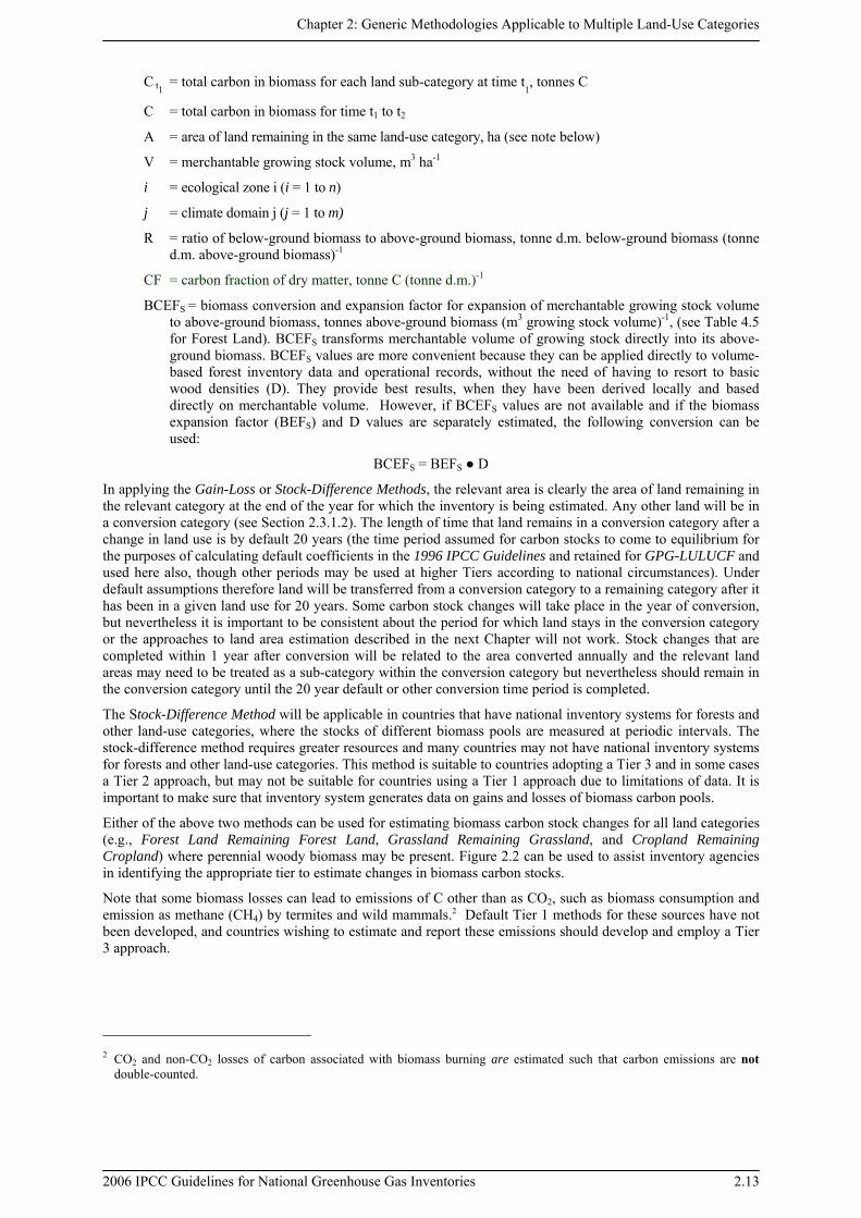
BCEFS = biomass conversion and expansion factor for expansion of merchantable growing stock volume to above-ground biomass, tonnes above-ground biomass (m3 growing stock volume)-1, (see Table 4.5 for Forest Land). BCEFS transforms merchantable volume of growing stock directly into its above-ground biomass. BCEFS values are more convenient because they can be applied directly to volume-based forest inventory data and operational records, without the need of having to resort to basic wood densities (D). They provide best results, when they have been derived locally and based directly on merchantable volume. However, if BCEFS values are not available and if the biomass expansion factor (BEFS) and D values are separately estimated, the following conversion can be used:

BCEFS = BEFS ● D

In applying the Gain-Loss or Stock-Difference Methods, the relevant area is clearly the area of land remaining in the relevant category at the end of the year for which the inventory is being estimated. Any other land will be in a conversion category (see Section 2.3.1.2). The length of time that land remains in a conversion category after a change in land use is by default 20 years (the time period assumed for carbon stocks to come to equilibrium for the purposes of calculating default coefficients in the 1996 IPCC Guidelines and retained for GPG-LULUCF and used here also, though other periods may be used at higher Tiers according to national circumstances). Under default assumptions therefore land will be transferred from a conversion category to a remaining category after it has been in a given land use for 20 years. Some carbon stock changes will take place in the year of conversion, but nevertheless it is important to be consistent about the period for which land stays in the conversion category or the approaches to land area estimation described in the next Chapter will not work. Stock changes that are completed within 1 year after conversion will be related to the area converted annually and the relevant land areas may need to be treated as a sub-category within the conversion category but nevertheless should remain in the conversion category until the 20 year default or other conversion time period is completed.

The Stock-Difference Method will be applicable in countries that have national inventory systems for forests and other land-use categories, where the stocks of different biomass pools are measured at periodic intervals. The stock-difference method requires greater resources and many countries may not have national inventory systems for forests and other land-use categories. This method is suitable to countries adopting a Tier 3 and in some cases a Tier 2 approach, but may not be suitable for countries using a Tier 1 approach due to limitations of data. It is important to make sure that inventory system generates data on gains and losses of biomass carbon pools.

Either of the above two methods can be used for estimating biomass carbon stock changes for all land categories (e.g., Forest Land Remaining Forest Land, Grassland Remaining Grassland, and Cropland Remaining Cropland) where perennial woody biomass may be present. Figure 2.2 can be used to assist inventory agencies in identifying the appropriate tier to estimate changes in biomass carbon stocks.

Note that some biomass losses can lead to emissions of C other than as CO2, such as biomass consumption and emission as methane (CH4) by termites and wild mammals.2 Default Tier 1 methods for these sources have not been developed, and countries wishing to estimate and report these emissions should develop and employ a Tier 3 approach.

2 CO2 and non-CO2 losses of carbon associated with biomass burning are estimated such that carbon emissions are not

double-counted.



Figure 2.2 Generic decision tree for identification of appropriate tier to estimate changes in carbon stocks in biomass in a land-use category.

Start

Are detaileddata on biomass

available to estimate changes in C stocks using dynamic models or

allometricequations?

Are country-specific biomass data

and emission/removal factorsavailable?

Are changesin C stocks in biomass in

this land classification a keycategory1?

Areaggregate data on

biomass growth andloss available?

Collect data for the Tier3 or Tier 2 method.

Gather data onbiomass growth

and biomass loss.

Use the detailed biomass data for Tier 3 method.

Use country-specificbiomass data and

emission/removal factorsfor the Tier 2 method.

Use aggregate data anddefault emission/removalfactors for Tier 1 method.

Yes

No

Yes

No

Yes

No

Yes

Box 3: Tier 3

Box 2: Tier 2

Box 1: Tier 1

No

Note:1: See Volume 1 Chapter 4, "Methodological Choice and Identification of Key Categories" (noting Section 4.1.2 on limited resources), for discussion of key categories and use of decision trees.



A. METHODS FOR ESTIMATING CHANGE IN CARBON STOCKS IN BIOMASS (∆CB)

A.1 Estimating annual increase in biomass carbon stocks (Gain-Loss Method), ∆CG

This is the Tier 1 method that, when combined with default biomass growth rates, allows for any country to calculate the annual increase in biomass, using estimates of area and mean annual biomass increment, for each land-use type and stratum (e.g., climatic zone, ecological zone, vegetation type) (Equation 2.9).

EQUATION 2.9 ANNUAL INCREASE IN BIOMASS CARBON STOCKS DUE TO BIOMASS INCREMENT

IN LAND REMAINING IN THE SAME LAND-USE CATEGORY ∑ ••=Δ

jijiTOTALjiG CFGAC

ji,

,, )(,

Where:

∆CG = annual increase in biomass carbon stocks due to biomass growth in land remaining in the same land-use category by vegetation type and climatic zone, tonnes C yr-1

A = area of land remaining in the same land-use category, ha

GTOTAL= mean annual biomass growth, tonnes d. m. ha-1 yr-1

i = ecological zone (i = 1 to n)

j = climate domain (j = 1 to m)


GTOTAL is the total biomass growth expanded from the above-ground biomass growth (Gw) to include below-ground biomass growth. Following a Tier 1 method, this may be achieved directly by using default values of GW for naturally regenerated trees or broad categories of plantations together with R, the ratio of below-ground biomass to above-ground biomass differentiated by woody vegetation type. In Tiers 2 and 3, the net annual increment (IV) can be used with either basic wood density (D) and biomass expansion factor (BEFI) or directly with biomass conversion and expansion factor (BCEFI) for conversion of annual net increment to above-ground biomass increment for each vegetation type. Equation 2.10 shows the relationships.

EQUATION 2.10 AVERAGE ANNUAL INCREMENT IN BIOMASS

Tier 1 ∑ +•= )}1({ RGG WTOTAL Biomass increment data (dry matter) are used directly

Tiers 2 and 3 ∑ +••= )}1({ RBCEFIG IVTOTAL Net annual increment data are used to estimate GW by

applying a biomass conversion and expansion factor

Where:

GTOTAL = average annual biomass growth above and below-ground, tonnes d. m. ha-1 yr-1

GW = average annual above-ground biomass growth for a specific woody vegetation type, tonnes d. m. ha-1 yr-1

R = ratio of below-ground biomass to above-ground biomass for a specific vegetation type, in tonne d.m. below-ground biomass (tonne d.m. above-ground biomass)-1. R must be set to zero if assuming no changes of below-ground biomass allocation patterns (Tier 1).

IV = average net annual increment for specific vegetation type, m3 ha-1 yr-1

BCEFI = biomass conversion and expansion factor for conversion of net annual increment in volume (including bark) to above-ground biomass growth for specific vegetation type, tonnes above-ground biomass growth (m3 net annual increment)-1, (see Table 4.5 for Forest Land). If BCEFI values are not



available and if the biomass expansion factor (BEF) and basic wood density (D) values are separately estimated, then the following conversion can be used:

BCEFI = BEFI ● D

Biomass Expansion Factors (BEFI)3 expand merchantable volume to total above-ground biomass volume to account for non-merchantable components of increment. BEFI is dimensionless.

Estimates for BCEFI for woody (perennial) biomass on non-forest lands such as Grassland (savanna), Cropland (agro-forestry), orchards, coffee, tea, and rubber may not be readily available. In this case, default values of BCEFI from one of the forest types closest to the non-forest vegetation can be used to convert merchantable biomass to total biomass. BCEFI is relevant only to perennial woody tree biomass for which merchantable biomass data are available. For perennial shrubs, grasses and crops, biomass increment data in terms of tonnes of dry matter per hectare may be directly available and in this case use of Equation 2.10 will not be required.

A.2 Estimating annual decrease in biomass carbon stocks due to losses (Gain-Loss Method), ∆C

L

Loss estimates are needed for calculating biomass carbon stock change using the Gain-Loss Method. Note that the loss estimate is also needed when using the Stock–Difference Method to estimate the transfers of biomass to dead organic matter when higher Tier estimation methods are used (see below). Annual biomass loss is the sum of losses from wood removal (harvest), fuelwood removal (not counting fuelwood gathered from woody debris), and other losses resulting from disturbances, such as fire, storms, and insect and diseases. The relationship is shown in Equation 2.11.

EQUATION 2.11 ANNUAL DECREASE IN CARBON STOCKS DUE TO BIOMASS LOSSES

IN LAND REMAINING IN THE SAME LAND-USE CATEGORY

edisturbancfuelwoodremovalswoodL LLLC ++=Δ −

Where: ∆C

L = annual decrease in carbon stocks due to biomass loss in land remaining in the same land-use category, tonnes C yr-1

Lwood-removals = annual carbon loss due to wood removals, tonnes C yr-1 (See Equation 2.12)

Lfuelwood = annual biomass carbon loss due to fuelwood removals, tonnes C yr-1 (See Equation 2.13)

Ldisturbance = annual biomass carbon losses due to disturbances, tonnes C yr-1 (See Equation 2.14)

Equation 2.11 and the following Equations 2.12 to 2.14 are directly applicable to Forest Land. These Equations (2.11 to 2.14) can also be used for estimating losses from Cropland and Grassland, if quantities of wood removal (harvesting), fuelwood removal, and loss due to disturbance are available for perennial woody biomass. In intensively managed as well as highly degraded croplands and grasslands, the perennial woody biomass loss is likely to be small. Default biomass carbon loss values for woody crop species are provided for the Tier 1 cropland methodology (see Table 5.1). It is important to note that wood-removal used in Equation 2.11 should be compared with the input to HWP in Chapter 12 for consistency.

The three terms on the right hand side of Equation 2.11 are obtained as follows:

Loss of biomass and carbon from wood removal (harvest ing), Lw o o d - r e m o v a l s The method for estimating the annual biomass carbon loss due to wood-removals is provided in Equation 2.12.

3 In some applications, BEFs are used to expand dry-weight of merchantable components or stem biomass to total biomass,

excluding or including roots, or convert and expand merchantable or stem volume to above-ground or total biomass (Somogyi et al., 2006). As used in this document, biomass expansion factors always transform dry-weight of merchantable components including bark to aboveground biomass, excluding roots.



EQUATION 2.12 ANNUAL CARBON LOSS IN BIOMASS OF WOOD REMOVALS

})1({ CFRBCEFHL Rremovalswood •+••=−

Where:

Lwood-removals = annual carbon loss due to biomass removals, tonnes C yr-1

H = annual wood removals, roundwood, m3 yr-1

R = ratio of below-ground biomass to above-ground biomass, in tonne d.m. below-ground biomass (tonne d.m. above-ground biomass)-1. R must be set to zero if assuming no changes of below-ground biomass allocation patterns (Tier 1).


BCEFR = biomass conversion and expansion factor for conversion of removals in merchantable volume to total biomass removals (including bark), tonnes biomass removal (m3 of removals)-1, (see Table 4.5 for Forest Land). However, if BCEFR values are not available and if the biomass expansion factor for wood removals (BEFR) and basic wood density (D) values are separately estimated, then the following conversion can be used:

BCEFR = BEFR ● D

If country-specific data on roundwood removals are not available, the inventory experts should use FAO statistics on wood harvest. FAO statistical data on wood harvest exclude bark. To convert FAO statistical wood harvest data without bark into merchantable wood removals including bark, multiply by default expansion factor of 1.15.

Loss of biomass and carbon from fuelwood removal, Lf u e l w o o d Fuelwood removal will often be comprised of two components. First, removal for fuelwood of living trees and parts of trees such as tops and branches, where the tree itself remains in the forest, will reduce the carbon in the biomass of growing stock and should be treated as biomass carbon loss. The second component is gathering of dead wood and logging slash. This will reduce the dead organic matter carbon pool. If it is possible it is good practice to estimate the two components separately. The biomass carbon loss due to fuelwood removal of live trees is estimated using Equation 2.13.

EQUATION 2.13 ANNUAL CARBON LOSS IN BIOMASS OF FUELWOOD REMOVAL

CFDFGRBCEFFGL partRtreesfuelwood ••++••= ])}1([{

Where:

Lfuelwood = annual carbon loss due to fuelwood removals, tonnes C yr-1

FGtrees = annual volume of fuelwood removal of whole trees, m3 yr-1

FGpart = annual volume of fuelwood removal as tree parts, m3 yr-1

R = ratio of below-ground biomass to above-ground biomass, in tonne d.m. below-ground biomass (tonne d.m. above-ground biomass)-1; R must be set to zero if assuming no changes of below-ground biomass allocation patterns. (Tier 1)


D = basic wood density, tonnes d.m. m-3

BCEFR = biomass conversion and expansion factor for conversion of removals in merchantable volume to biomass removals (including bark), tonnes biomass removal (m3 of removals)-1, (see Table 4.5 for Forest Land). If BCEFR values are not available and if the biomass expansion factor for wood removals (BEFR) and basic wood density (D) values are separately estimated, then the following conversion can be used:

BCEFR = BEFR ● D

Biomass Expansion Factors (BEFR) expand merchantable wood removals to total aboveground biomass volume to account for non-merchantable components of the tree, stand and forest. BEFR is dimensionless.



If country-specific data on roundwood removals are not available, the inventory experts should use FAO statistics on wood harvest. It should be noted that FAO statistical data on wood harvest exclude bark. To convert FAO statistical wood harvest data without bark into merchantable wood removals including bark, multiply by default expansion factor of 1.15.

Wood harvest can comprise both wood and fuelwood removals (i.e., wood removals in Equation 2.12 can include both wood and fuelwood removal), or fuelwood removals can be reported separately using, both Equations 2.12 and 2.13. To avoid double counting, it is good practice to check how fuelwood data are represented in the country and to use the equation that is most appropriate for national conditions. Furthermore, the wood harvest from forests becomes an input to HWP (Chapter 12). Therefore, it is good practice to check for consistent representation of wood-harvest data in Equations 2.12 and 2.13 and those in Chapter 12.

Loss of biomass and carbon from disturbance, Ld i s t u r b a n c e A generic approach for estimating the amount of carbon lost from disturbances is provided in Equation 2.14. In the specific case of losses from fire on managed land, including wildfires and controlled fires, this method should be used to provide input to the methodology to estimate CO2 and non-CO2 emissions from fires.

EQUATION 2.14 ANNUAL CARBON LOSSES IN BIOMASS DUE TO DISTURBANCES

})1({ fdCFRBAL Wedisturbancedisturbanc ••+••=

Where:

Ldisturbances = annual other losses of carbon, tonnes C yr-1 (Note that this is the amount of biomass that is lost from the total biomass. The partitioning of biomass that is transferred to dead organic matter and biomass that is oxidized and released to the atmosphere is explained in Equations 2.15 and 2.16).

Adisturbance = area affected by disturbances, ha yr-1

BW = average above-ground biomass of land areas affected by disturbances, tonnes d.m. ha-1

R = ratio of below-ground biomass to above-ground biomass, in tonne d.m. below-ground biomass (tonne d.m. above-ground biomass)-1. R must be set to zero if no changes of below-ground biomass are assumed (Tier 1)

CF = carbon fraction of dry matter, tonne C (tonnes d.m.)-1

fd = fraction of biomass lost in disturbance (see note below)

Note: The parameter fd defines the proportion of biomass that is lost from the biomass pool: a stand-replacing disturbance will kill all (fd = 1) biomass while an insect disturbance may only remove a portion (e.g. fd = 0.3) of the average biomass C density. Equation 2.14 does not specify the fate of the carbon removed from the biomass carbon stock. The Tier 1 assumption is that all of Ldisturbances is emitted in the year of disturbance. Higher Tier methods assume that some of this carbon is emitted immediately and some is added to the dead organic matter pools (dead wood, litter) or HWP.

The amounts of biomass carbon transferred to different fates can be defined using a disturbance matrix that can be parameterized to define the impacts of different disturbance types (Kurz et al., 1992). It is good practice, if possible, to develop and use a disturbance matrix (Table 2.1) for each biomass, dead organic matter and soil carbon pool, the proportion of the carbon remaining in that pool, and the proportions transferred to other pools, to harvested wood products and to the atmosphere, during the disturbance event. The proportions in each row always sum to 1 to ensure conservation of carbon. The value entered in cell A is the proportion of above-ground biomass remaining after a disturbance (or 1 – fd, where fd is defined in Equation 2.14). The Tier 1 assumption is that all of fd is emitted in the year of disturbance: therefore the value entered in cell F is fd. For higher Tiers, only the proportion emitted in the year is entered in cell F and the remainder is added to cells B and C in the case of fire, and B, C, and E in the case of harvest. It is good practice to develop disturbance matrix even under Tier 1 to ensure that all carbon pool transfers are considered, though all biomass carbon is assumed to be emitted in the year of land conversion. It is important to note that some of the transfers could be small or insignificant.



TABLE 2.1 EXAMPLE OF A SIMPLE MATRIX (TIER 2) FOR THE IMPACTS OF DISTURBANCES ON CARBON POOLS

To:

From:

Above-ground biomass

Below-ground biomass

Dead wood

Litter Soil organic matter

Harvested wood

products

Atmo-sphere

Sum of row

(must equal 1)

Above-ground biomass

A B C D E F 1

Below-ground biomass

1

Dead wood 1

Litter 1

Soil organic matter

1

Enter the proportion of each pool on the left side of the matrix that is transferred to the pool at the top of each column. All of the pools on the left side of the matrix must be fully populated and the values in each row must sum to 1. Impossible transitions are blacked out. Note: Letters A to F are cell labels that are referenced in the text.

2.3.1.2 LAND CONVERTED TO A NEW LAND-USE CATEGORY The methods for estimation of emissions and removals of carbon resulting from land-use conversion from one land-use category to another are presented in this section. Possible conversions include conversion from non-forest to Forest Land, Cropland and Forest Land to Grassland, and Grassland and Forest Land to Cropland.

The CO2 emissions and removals on land converted to a new land-use category include annual changes in carbon stocks in above-ground and below-ground biomass. Annual carbon stock changes for each of these pools can be estimated by using Equation 2.4 (ΔCB = ∆CG - ∆CL), where ∆CG is the annual gain in carbon, and ∆CL is the annual loss of carbon. ΔCB can be estimated separately for each land use (e.g., Forest Land, Cropland, Grassland) and management category (e.g., natural forest, plantation), by specific strata (e.g., climate or forest type).

METHODS FOR ESTIMATING CHANGE IN CARBON STOCKS IN BIOMASS (∆CB)

i) Annual increase in carbon stocks in biomass, ∆CG Tier 1: Annual increase in carbon stocks in biomass due to land converted to another land-use category can be estimated using Equation 2.9 described above for lands remaining in a category. Tier 1 employs a default assumption that there is no change in initial biomass carbon stocks due to conversion. This assumption can be applied if the data on previous land uses are not available, which may be the case when land area totals are estimated using Approach 1 or 2 described in Chapter 3 (non-spatially explicit land area data). This approach implies the use of default parameters in Section 4.5 (Chapter 4). The area of land converted can be categorized based on management practices e.g., intensively managed plantations and grasslands or extensively managed (low input) plantations, grasslands or abandoned croplands that revert back to forest and should be kept in conversion category for 20 years or another time interval. If the previous land use on a converted area is known, then the Tier 2 method described below can be used.

i i ) Annual decrease in carbon stocks in biomass due to losses, ∆CL Tier 1: The annual decrease in C stocks in biomass due to losses on converted land (wood removals or fellings, fuelwood collection, and disturbances) can be estimated using Equations 2.11 to 2.14. As with increases in carbon stocks, Tier 1 follows the default assumption that there is no change in initial carbon stocks in biomass, and it can be applied for the areas that are estimated with the use of Approach 1 or 2 in Chapter 3, and default parameters in Section 4.5.



i i i ) Higher tiers for estimating change in carbon stocks in biomass, (∆CB) Tiers 2 and 3: Tier 2 (and 3) methods use nationally-derived data and more disaggregated approaches and (or) process models, which allow for more precise estimates of changes in carbon stocks in biomass. In Tier 2, Equation 2.4 is replaced by Equation 2.15, where the changes in carbon stock are calculated as a sum of increase in carbon stock due to biomass growth, changes due to actual conversion (difference between biomass stocks before and after conversion), and decrease in carbon stocks due to losses.

EQUATION 2.15 ANNUAL CHANGE IN BIOMASS CARBON STOCKS ON LAND CONVERTED TO OTHER LAND-USE

CATEGORY (TIER 2)

LCONVERSIONGB CCCC Δ−Δ+Δ=Δ

Where:

∆CB = annual change in carbon stocks in biomass on land converted to other land-use category, in tonnes C yr-1

∆CG = annual increase in carbon stocks in biomass due to growth on land converted to another land-use category, in tonnes C yr-1

∆CCONVERSION

= initial change in carbon stocks in biomass on land converted to other land-use category, in tonnes C yr-1

∆CL = annual decrease in biomass carbon stocks due to losses from harvesting, fuel wood gathering and disturbances on land converted to other land-use category, in tonnes C yr-1

Conversion to another land category may be associated with a change in biomass stocks, e.g., part of the biomass may be withdrawn through land clearing, restocking or other human-induced activities. These initial changes in carbon stocks in biomass (∆C

CONVERSION) are calculated with the use of Equation 2.16 as follows:

EQUATION 2.16 INITIAL CHANGE IN BIOMASS CARBON STOCKS ON LAND CONVERTED TO ANOTHER LAND

CATEGORY ∑ •Δ•−=Δi

OTHERSTOBEFOREAFTERCONVERSION CFABBCiii}){( _

Where:

∆CCONVERSION

= initial change in biomass carbon stocks on land converted to another land category, tonnes C yr-1

BAFTERi = biomass stocks on land type i immediately after the conversion, tonnes d.m. ha-1

BBEFOREi = biomass stocks on land type i before the conversion, tonnes d.m. ha-1

∆ATO_OTHERSi = area of land use i converted to another land-use category in a certain year, ha yr-1

CF = carbon fraction of dry matter, tonne C (tonnes d.m.)-1

i = type of land use converted to another land-use category

The calculation of ∆CCONVERSION

may be applied separately to estimate carbon stocks occurring on specific types of land (ecosystems, site types, etc.) before the conversion. The ∆ATO_OTHERSi

refers to a particular inventory year for which the calculations are made, but the land affected by conversion should remain in the conversion category for 20 years or other period used in the inventory. Inventories using higher Tier methods can define a disturbance matrix (Table 2.1) for land-use conversion to quantify the proportion of each carbon pool before conversion that is transferred to other pools, emitted to the atmosphere (e.g., slash burning), or otherwise removed during harvest or land clearing.



Owing to the use of country specific data and more disaggregated approaches, the Equations 2.15 and 2.16 provide for more accurate estimates than Tier 1 methods, where default data are used. Additional improvement or accuracy would be achieved by using national data on areas of land-use transitions and country-specific carbon stock values. Therefore, Tier 2 and 3 approaches should be inclusive of estimates that use detailed area data and country specific carbon stock values.

2.3.2 Change in carbon stocks in dead organic matter Dead organic matter (DOM) comprises dead wood and litter (See Table 1.1). Estimating the carbon dynamics of dead organic matter pools allows for increased accuracy in the reporting of where and when carbon emissions and removals occur. For example, only some of the carbon contained in biomass killed during a biomass burning is emitted into the atmosphere in the year of the fire. Most of the biomass is added to dead wood, litter and soil pools (dead fine roots are included in the soil) from where the C will be emitted over years to decades, as the dead organic matter decomposes. Decay rates differ greatly between regions, ranging from high in warm and moist environments to low in cold and dry environments. Although the carbon dynamics of dead organic matter pools are well understood qualitatively, countries may find it difficult to obtain actual data with national coverage on dead organic matter stocks and their dynamics.

In forest ecosystems, DOM pools tend to be largest following stand-replacing disturbances due to the addition of residual above-ground and below-ground (roots) biomass. In the years after the disturbance, DOM pools decline as carbon loss through decay exceeds the rate of carbon addition through litterfall, mortality and biomass turnover. Later in stand development, DOM pools increase again. Representing these dynamics requires separate estimation of age-dependent inputs and outputs associated with stand dynamics and disturbance-related inputs and losses. These more complex estimation procedures require higher Tier methods.

2.3.2.1 LAND REMAINING IN A LAND-USE CATEGORY The Tier 1 assumption for both dead wood and litter pools for all land-use categories is that their stocks are not changing over time if the land remains within the same land-use category. Thus, the carbon in biomass killed during a disturbance or management event (less removal of harvested wood products) is assumed to be released entirely to the atmosphere in the year of the event. This is equivalent to the assumption that the carbon in non-merchantable and non-commercial components that are transferred to dead organic matter is equal to the amount of carbon released from dead organic matter to the atmosphere through decomposition and oxidation. Countries can use higher tier methods to estimate the carbon dynamics of dead organic matter. This section describes estimation methods if Tier 2 (or 3) methods are used.

Countries that use Tier 1 methods to estimate DOM pools in land remaining in the same land-use category, report zero changes in carbon stocks or carbon emissions from those pools. Following this rule, CO2 emissions resulting from the combustion of dead organic matter during fire are not reported, nor are the increases in dead organic matter carbon stocks in the years following fire. However, emissions of non-CO2 gases from burning of DOM pools are reported. Tier 2 methods for estimation of carbon stock changes in DOM pools calculate the changes in dead wood and litter carbon pools (Equation 2.17). Two methods can be used: either track inputs and outputs (the Gain-Loss Method, Equation 2.18) or estimate the difference in DOM pools at two points in time (Stock-Difference Method, Equation 2.19). These estimates require either detailed inventories that include repeated measurements of dead wood and litter pools, or models that simulate dead wood and litter dynamics. It is good practice to ensure that such models are tested against field measurements and are documented. Figure 2.3 provides the decision tree for identification of the appropriate tier to estimate changes in carbon stocks in dead organic matter.

Equation 2.17 summarizes the calculation to estimate the annual changes in carbon stock in DOM pools:

EQUATION 2.17 ANNUAL CHANGE IN CARBON STOCKS IN DEAD ORGANIC MATTER

LTDWDOM CCC Δ+Δ=Δ

Where:

∆CDOM

= annual change in carbon stocks in dead organic matter (includes dead wood and litter), tonnes C yr-1

∆CDW

= change in carbon stocks in dead wood, tonnes C yr-1

∆CLT

= change in carbon stocks in litter, tonnes C yr-1



Figure 2.3 Generic decision tree for identification of appropriate tier to estimate changes in carbon stocks in dead organic matter for a land-use category

Start

Are data onmanaged area and DOM stocks

at two periods of time available toestimate changes

in C stocks?

Are data onmanaged area and annual

transfer into and out of DOM stocks available?

Are changes in C stocks in DOM a key category1?

Collect data for Tier 2method (Gain-LossMethod or Stock-

Difference Method2).

Use the data for Tier 2method (Stock-

Difference Method) orTier 3 Method.

Use the data for Tier 2method (Gain-LossMethod) or Tier 3

Method.

Assume that the deadorganic matter stock is

in equilibrium.

Yes

No

Yes

No

Yes

Box 3: Tier 2

Box 2: Tier 2

Box 1: Tier 1

No

Note:1: See Volume 1 Chapter 4, "Methodological Choice and Identification of Key Categories" (noting Section 4.1.2 on limited resources), for discussion of key categories and use of decision trees.2: The two methods are defined in Equations 2.18 and 2.19, respectively.



The changes in carbon stocks in the dead wood and litter pools for an area remaining in a land-use category between inventories can be estimated using two methods, described in Equation 2.18 and Equation 2.19. The same equation is used for dead wood and litter pools, but their values are calculated separately.

EQUATION 2.18 ANNUAL CHANGE IN CARBON STOCKS IN DEAD WOOD OR LITTER (GAIN-LOSS METHOD)

}){( CFDOMDOMAC outinDOM •−•=Δ

Where:

∆C DOM = annual change in carbon stocks in the dead wood/litter pool, tonnes C yr-1

A = area of managed land, ha

DOMin = average annual transfer of biomass into the dead wood/litter pool due to annual processes and disturbances, tonnes d.m. ha-1 yr-1 (see next Section for further details).

DOMout = average annual decay and disturbance carbon loss out of dead wood or litter pool, tonnes d.m. ha-1 yr-1


The net balance of DOM pools specified in Equation 2.18, requires the estimation of both the inputs and outputs from annual processes (litterfall and decomposition) and the inputs and losses associated with disturbances. In practice, therefore, Tier 2 and Tier 3 approaches require estimates of the transfer and decay rates as well as activity data on harvesting and disturbances and their impacts on DOM pool dynamics. Note that the biomass inputs into DOM pools used in Equation 2.18 are a subset of the biomass losses estimated in Equation 2.7. The biomass losses in Equation 2.7 contain additional biomass that is removed from the site through harvest or lost to the atmosphere, in the case of fire.

The method chosen depends on available data and will likely be coordinated with the method chosen for biomass carbon stocks. Transfers into and out of a dead wood or litter pool for Equation 2.18 may be difficult to estimate. The stock difference method described in Equation 2.19 can be used by countries with forest inventory data that include DOM pool information, other survey data sampled according to the principles set out in Annex 3A.3 (Sampling) in Chapter 3, and/or models that simulate dead wood and litter dynamics.

EQUATION 2.19 ANNUAL CHANGE IN CARBON STOCKS IN DEAD WOOD OR LITTER (STOCK-DIFFERENCE

METHOD)

CFT

DOMDOMAC tt

DOM •⎥⎦

⎤⎢⎣

⎡ −•=Δ

)(12

Where:

∆CDOM

= annual change in carbon stocks in dead wood or litter, tonnes C yr-1

A = area of managed land, ha

DOMt1 = dead wood/litter stock at time t1 for managed land, tonnes d.m. ha-1

DOMt2 = dead wood/litter stock at time t2 for managed land, tonnes d.m. ha-1

T = (t2 – t1) = time period between time of the second stock estimate and the first stock estimate, yr

CF = carbon fraction of dry matter (default = 0.37 for litter), tonne C (tonne d.m.)-1

Note that whenever the stock change method is used (e.g., in Equation 2.19), the area used in the carbon stock calculations at times t1 and t2 must be identical. If the area is not identical then changes in area will confound the estimates of carbon stocks and stock changes. It is good practice to use the area at the end of the inventory period (t2) to define the area of land remaining in the land-use category. The stock changes on all areas that change land-use category between t1 and t2 are estimated in the new land-use category, as described in the sections on land converted to a new land category.

INPUT OF BIOMASS TO DEAD ORGANIC MATTER Whenever a tree is felled, non-merchantable and non-commercial components (such as tops, branches, leaves, roots, and noncommercial trees) are left on the ground and transferred to dead organic matter pools. In addition,



annual mortality can add substantial amounts of dead wood to that pool. For Tier 1 methods, the assumption is that the carbon contained in all biomass components that are transferred to dead organic matter pools will be released in the year of the transfer, whether from annual processes (litterfall and tree mortality), land management activities, fuelwood gathering, or disturbances. For estimation procedures based on higher Tiers, it is necessary to estimate the amount of biomass carbon that is transferred to dead organic matter. The quantity of biomass transferred to DOM is estimated using Equation 2.20.

EQUATION 2.20 ANNUAL CARBON IN BIOMASS TRANSFERRED TO DEAD ORGANIC MATTER

)}({ BLoledisturbancslashmortalityin fLLLDOM •++=

Where:

DOMin = total carbon in biomass transferred to dead organic matter, tonnes C yr-1

Lmortality = annual biomass carbon transfer to DOM due to mortality, tonnes C yr-1 (See Equation 2.21)

Lslash = annual biomass carbon transfer to DOM as slash, tonnes C yr-1 (See Equations 2.22)

Ldisturbances = annual biomass carbon loss resulting from disturbances, tonnes C yr-1 (See Equation 2.14)

fBLol = fraction of biomass left to decay on the ground (transferred to dead organic matter) from loss due to disturbance. As shown in Table 2.1, the disturbance losses from the biomass pool are partitioned into the fractions that are added to dead wood (cell B in Table 2.1) and to litter (cell C), are released to the atmosphere in the case of fire (cell F) and, if salvage follows the disturbance, transferred to HWP (cell E).

Note: If root biomass increments are counted in Equation 2.10, then root biomass losses must also be counted in Equations 2.20, and 2.22.

Examples of the terms on the right hand side of Equation 2.20 are obtained as follows:

Transfers to dead organic matter from mortali ty, Lm o r t a l i t y Mortality is caused by competition during stand development, age, diseases, and other processes that are not included as disturbances. Mortality cannot be neglected when using higher Tier estimation methods. In extensively managed stands without periodic partial cuts, mortality from competition during the stem exclusion phase, may represent 30-50% of total productivity of a stand during its lifetime. In regularly tended stands, additions to the dead organic matter pool from mortality may be negligible because partial cuts extract forest biomass that would otherwise be lost to mortality and transferred to dead organic matter pools. Available data for increment will normally report net annual increment, which is defined as net of losses from mortality. Since in this text, net annual growth is used as a basis to estimate biomass gains, mortality must not be subtracted again as a loss from biomass pools. Mortality must, however, be counted as an addition to the dead wood pool for Tier 2 and Tier 3 methods.

The equation for estimating mortality is provided in Equation 2.21:

EQUATION 2.21 ANNUAL BIOMASS CARBON LOSS DUE TO MORTALITY

∑ •••= )( mCFGAL Wmortality

Where:

Lmortality = annual biomass carbon loss due to mortality, tonnes C yr-1

A = area of land remaining in the same land use, ha

Gw = above-ground biomass growth, tonnes d.m. ha-1 yr-1 (see Equation 2.10)


m = mortality rate expressed as a fraction of above-ground biomass growth



When data on mortality rates are expressed as proportion of growing stock volume, then the term Gw in Equation 2.21 should be replaced with growing stock volume to estimate annual transfer to DOM pools from mortality.

Mortality rates differ between stages of stand development and are highest during the stem exclusion phase of stand development. They also differ with stocking level, forest type, management intensity and disturbance history. Thus, providing default values for an entire climatic zone is not justified because the variation within a zone will be much larger than the variation between zones.

Annual carbon transfer to slash, L s l a s h This involves estimating the quantity of slash left after wood removal or fuelwood removal and transfer of biomass from total annual carbon loss due to wood harvest (Equation 2.12). The estimate for logging slash is given in Equation 2.22 and which is derived from Equation 2.12 as explained below:

EQUATION 2.22 ANNUAL CARBON TRANSFER TO SLASH

{ } { }[ ] CFDHRBCEFHL Rslash ••−+••= )1(

Where:

Lslash = annual carbon transfer from above-ground biomass to slash, including dead roots, tonnes C yr-1

H = annual wood harvest (wood or fuelwood removal), m3 yr-1

BCEFR = biomass conversion and expansion factors applicable to wood removals, which transform merchantable volume of wood removal into above-ground biomass removals, tonnes biomass removal (m3 of removals)-1. If BCEFR values are not available and if BEF and Density values are separately estimated then the following conversion can be used:

BCEFR = BEFR ● D

o D is basic wood density, tonnes d.m. m-3

o Biomass Expansion Factors (BEFR) expand merchantable wood removals to total aboveground biomass volume to account for non-merchantable components of the tree, stand and forest. BEFR is dimensionless.

R = ratio of below-ground biomass to above-ground biomass, in tonne d.m. below-ground biomass (tonne d.m. above-ground biomass)-1. R must be set to zero if root biomass increment is not included in Equation 2.10 (Tier 1)


Fuelwood gathering that involves the removal of live tree parts does not generate any additional input of biomass to dead organic matter pools and is not further addressed here.

Inventories using higher Tier methods can also estimate the amount of logging slash remaining after harvest by defining the proportion of above-ground biomass that is left after harvest (enter these proportions in cells B and C of Table 2.1 for harvest disturbance) and by using the approach defined in Equation 2.14. In this approach, activity data for the area harvested would also be required.

2.3.2.2 LAND CONVERSION TO A NEW LAND-USE CATEGORY The reporting convention is that all carbon stock changes and non-CO2 greenhouse gas emissions associated with a land-use change be reported in the new land-use category. For example, in the case of conversion of Forest Land to Cropland, both the carbon stock changes associated with the clearing of the forest as well as any subsequent carbon stock changes that result from the conversion are reported under the Cropland category.

The Tier 1 assumption is that DOM pools in non-forest land categories after the conversion are zero, i.e., they contain no carbon. The Tier 1 assumption for land converted from forest to another land-use category is that all DOM carbon losses occur in the year of land-use conversion. Conversely, conversion to Forest Land results in buildup of litter and dead wood carbon pools starting from zero carbon in those pools. DOM carbon gains on land converted to forest occur linearly, starting from zero, over a transition period (default assumption is 20 years). This default period may be appropriate for litter carbon stocks, but in temperate and boreal regions it is probably too short for dead wood carbon stocks. Countries that use higher Tier methods can accommodate



longer transition periods by subdividing the remaining category to accommodate strata that are in the later stages of transition.

The estimation of carbon stock changes during transition periods following land-use conversion requires that annual cohorts of the area subject to land-use change be tracked for the duration of the transition period. For example, DOM stocks are assumed to increase for 20 years after conversion to Forest Land. After 20 years, the area converted enters the category Forest Land Remaining Forest Land, and no further DOM changes are assumed, if a Tier 1 approach is applied. Under Tier 2 and 3, the period of conversion can be varied depending on vegetation and other factors that determine the time required for litter and dead wood pools to reach steady state.

Higher Tier estimation methods can use non-zero estimates of litter and dead wood pools in the appropriate land-use categories or subcategories. For example, settlements and agro-forestry systems can contain some litter and dead wood pools, but because management, site conditions, and many other factors influence the pool sizes, no global default values can be provided here. Higher Tier methods may also estimate the details of dead organic matter inputs and outputs associated with the land-use change.

The conceptual approach to estimating changes in carbon stocks in dead wood and litter pools is to estimate the difference in C stocks in the old and new land-use categories and to apply this change in the year of the conversion (carbon losses), or to distribute it uniformly over the length of the transition period (carbon gains) Equation 2.23:

EQUATION 2.23 ANNUAL CHANGE IN CARBON STOCKS IN DEAD WOOD AND LITTER DUE TO LAND CONVERSION

on

ononDOM T

ACCC •−=Δ

)(

Where:

∆CDOM

= annual change in carbon stocks in dead wood or litter, tonnes C yr-1

Co = dead wood/litter stock, under the old land-use category, tonnes C ha-1

Cn = dead wood/litter stock, under the new land-use category, tonnes C ha-1

Aon = area undergoing conversion from old to new land-use category, ha

Ton = time period of the transition from old to new land-use category, yr. The Tier 1 default is 20 years for carbon stock increases and 1 year for carbon losses.

Inventories using a Tier 1 method assume that all carbon contained in biomass killed during a land-use conversion event (less harvested products that are removed) is emitted directly to the atmosphere and none is added to dead wood and litter pools. Tier 1 methods also assume that dead wood and litter pool carbon losses occur entirely in the year of the transition.

Countries using higher Tier methods can modify Co in Equation 2.23 by first accounting for the immediate effects of the land-use conversion in the year of the event. In this case, they would add to Co the carbon from biomass killed and transferred to the dead wood and litter pools and remove from Co any carbon released from dead wood and litter pools, e.g., during slash burning. In that case Co in Equation 2.23 would represent the dead wood or litter carbon stocks immediately after the land-use conversion. Co will transit to Cn over the transition period, using linear or more complex dynamics. A disturbance matrix (Table 2.1) can be defined to account for the pool transitions and releases during the land-use conversion, including the additions and removals to Co.

Countries using a Tier 1 approach can apply the Tier 1 default carbon stock estimates for litter, and if available dead wood pools, provided in Table 2.2, but should recognize that these are broad-scale estimates with considerable uncertainty when applied at the country level. Table 2.2 is incomplete because of the paucity of published data. A review of the literature has identified several problems. The IPCC definitions of dead organic matter carbon stocks include litter and dead wood. The litter pool contains all litter plus fine woody debris up to a diameter limit of 10 cm (see Chapter 1, Table 1.1). Published litter data generally do not include the fine woody debris component, so the litter values in Table 2.2 are incomplete.

There are numerous published studies of coarse woody debris (Harmon and Hua, 1991; Karjalainen and Kuuluvainen, 2002) and a few review papers (e.g., Harmon et al., 1986), and but to date only two studies are found to provide regional dead wood carbon pool estimates that are based on sample plot data. Krankina et al. (2002) included several regions in Russia and reported coarse woody debris (> 10 cm diameter) estimates of 2 to



7 Mg C ha-1. Cooms et al. (2002) reported regional carbon pools based on a statistical sample design for a small region in New Zealand. Regional compilations for Canada (Shaw et al., 2005) provide estimates of litter carbon pools based on a compilation of statistically non-representative sample plots, but do not include estimates of dead wood pools. Review papers such as Harmon et al. (1986) compile a number of estimates from the literature. For example, their Table 5 lists a range of coarse woody debris values for temperate deciduous forests of 11 – 38 Mg dry matter ha-1 and for temperate coniferous forests of 10 – 511 Mg dry matter ha-1. It is, however, statistically invalid to calculate a mean from these compilations as they are not representative samples of the dead wood pools in a region.

While it is the intent of these IPCC Guidelines to provide default values for all variables used in Tier 1 methodologies, it is currently not feasible to provide estimates of regional defaults values for litter (including fine woody debris < 10 cm diameter) and dead wood (> 10 cm diameter) carbon stocks. Litter pool estimates (excluding fine woody debris) are provided in Table 2.2. Tier 1 methodology only requires the estimates in Table 2.2 for lands converted from Forest Land to any other land-use category (carbon losses) and for lands converted to Forest Land (carbon gains). Tier 1 methods assume that litter and dead wood pools are zero in all non-forest categories and therefore transitions between non-forest categories involve no carbon stock changes in these two pools.

TABLE 2.2 TIER 1 DEFAULT VALUES FOR LITTER AND DEAD WOOD CARBON STOCKS

Forest type

Broadleaf deciduous

Needleleaf evergreen

Broadleaf deciduous

Needleleaf evergreen

Litter carbon stocks of mature forests

Dead wood carbon stocks of mature forests

Climate

(tonnes C ha-1) (tonnes C ha-1)

Boreal, dry 25 (10 - 58)

31 (6 - 86) n.a.b n.a

Boreal, moist 39 (11 - 117)

55 (7 - 123) n.a n.a

Cold Temperate, dry 28 (23 - 33)a

27 (17 - 42) a n.a n.a

Cold temperate, moist 16 (5 - 31) a

26 (10 - 48) a n.a n.a

Warm Temperate, dry 28.2 (23.4 - 33.0)a

20.3 (17.3 - 21.1)a n.a n.a

Warm temperate, moist

13 (2 - 31) a

22 (6 - 42)a n.a n.a

Subtropical 2.8 (2 - 3) 4.1 n.a n.a

Tropical 2.1 (1 - 3) 5.2 n.a n.a

Source: Litter: Note that these values do not include fine woody debris. Siltanen et al., 1997; and Smith and Heath, 2001; Tremblay et al., 2002; and Vogt et al.,1996, converted from mass to carbon by multiplying by conversion factor of 0.37 (Smith and Heath, 2001). Dead Wood: No regional estimates of dead wood pools are currently available – see text for further comments a Values in parentheses marked by superscript “a” are the 5th and 95th percentiles from simulations of inventory

plots, while those without superscript “a” indicate the entire range. b n.a. denotes ‘not available’



2.3.3 Change in carbon stocks in soils Although both organic and inorganic forms of C are found in soils, land use and management typically has a larger impact on organic C stocks. Consequently, the methods provided in these guidelines focus mostly on soil organic C. Overall, the influence of land use and management on soil organic C is dramatically different in a mineral versus an organic soil type. Organic (e.g., peat and muck) soils have a minimum of 12 to 20 percent organic matter by mass (see Chapter 3 Annex 3A.5, for the specific criteria on organic soil classification), and develop under poorly drained conditions of wetlands (Brady and Weil, 1999). All other soils are classified as mineral soil types, and typically have relatively low amounts of organic matter, occurring under moderate to well drained conditions, and predominate in most ecosystems except wetlands. Discussion about land-use and management influences on these contrasting soil types is provided in the next two sections.

MINERAL SOILS Mineral soils are a carbon pool that is influenced by land-use and management activities. Land use can have a large effect on the size of this pool through activities such as conversion of native Grassland and Forest Land to Cropland, where 20-40% of the original soil C stocks can be lost (Mann, 1986; Davidson and Ackerman, 1993; Ogle et al., 2005). Within a land-use type, a variety of management practices can also have a significant impact on soil organic C storage, particularly in Cropland and Grassland (e.g., Paustian et al., 1997; Conant et al., 2001; Ogle et al., 2004 and 2005). In principle, soil organic C stocks can change with management or disturbance if the net balance between C inputs and C losses from soil is altered. Management activities influence organic C inputs through changes in plant production (such as fertilization or irrigation to enhance crop growth), direct additions of C in organic amendments, and the amount of carbon left after biomass removal activities, such as crop harvest, timber harvest, fire, or grazing. Decomposition largely controls C outputs and can be influenced by changes in moisture and temperature regimes as well as the level of soil disturbance resulting from the management activity. Other factors also influence decomposition, such as climate and edaphic characteristics. Specific effects of different land-use conversions and management regimes are discussed in the land-use specific chapters (Chapters 4 to 9).

Land-use change and management activity can also influence soil organic C storage by changing erosion rates and subsequent loss of C from a site; some eroded C decomposes in transport and CO2 is returned to the atmosphere, while the remainder is deposited in another location. The net effect of changing soil erosion through land management is highly uncertain, however, because an unknown portion of eroded C is stored in buried sediments of wetlands, lakes, river deltas and coastal zones (Smith et al., 2001).

ORGANIC SOILS Inputs of organic matter can exceed decomposition losses under anaerobic conditions, which are common in undrained organic soils, and considerable amounts of organic matter can accumulate over time. The carbon dynamics of these soils are closely linked to the hydrological conditions, including available moisture, depth of the water table, and reduction-oxidation conditions (Clymo, 1984; Thormann et al., 1999). Species composition and litter chemistry can also influence those dynamics (Yavitt et al., 1997).

Carbon stored in organic soils will readily decompose when conditions become aerobic following soil drainage (Armentano and Menges, 1986; Kasimir-Klemedtsson et al., 1997). Drainage is a practice used in agriculture and forestry to improve site conditions for plant growth. Loss rates vary by climate, with drainage under warmer conditions leading to faster decomposition rates. Losses of CO2 are also influenced by drainage depth; liming; the fertility and consistency of the organic substrate; and temperature (Martikainen et al., 1995). Greenhouse gas inventories capture this effect of management.

While drainage of organic soils typically releases CO2 to the atmosphere (Armentano and Menges, 1986), there can also be a decrease in emissions of CH4 that occur in un-drained organic soils (Nykänen et al., 1995). However, CH4 emissions from un-drained organic soils are not addressed in the inventory guidelines with the exception of a few cases in which the wetlands are managed (See Chapter 7, Wetlands). Similarly, national inventories typically do not estimate the accumulation of C in the soil pool resulting from the accumulation of plant detritus in un-drained organic soils. Overall, the rates of C gain are relatively slow in wetland environments with organic soils (Gorham, 1991), and any attempt to estimate C gains, even those created through wetland restoration, would also need to address the increase in CH4 emissions. See additional guidance in Chapter 7 Wetlands.



2.3.3.1 SOIL C ESTIMATION METHODS (LAND REMAINING IN A LAND-USE CATEGORY AND LAND CONVERSION TO A NEW LAND USE)

Soil C inventories include estimates of soil organic C stock changes for mineral soils and CO2 emissions from organic soils due to enhanced microbial decomposition caused by drainage and associated management activity. In addition, inventories can address C stock changes for soil inorganic C pools (e.g., calcareous grasslands that become acidified over time) if sufficient information is available to use a Tier 3 approach. The equation for estimating the total change in soil C stocks is given in Equation 2.24:

EQUATION 2.24 ANNUAL CHANGE IN CARBON STOCKS IN SOILS

InorganicOrganicMineralSoils CLCC Δ+−Δ=Δ

Where:

∆CSoils

= annual change in carbon stocks in soils, tonnes C yr-1

∆CMineral

= annual change in organic carbon stocks in mineral soils, tonnes C yr-1

LOrganic

= annual loss of carbon from drained organic soils, tonnes C yr-1

ΔCInorganic = annual change in inorganic carbon stocks from soils, tonnes C yr-1 (assumed to be 0 unless

using a Tier 3 approach)

For Tier 1 and 2 methods, soil organic C stocks for mineral soils are computed to a default depth of 30 cm. Greater depth can be selected and used at Tier 2 if data are available, but Tier 1 factors are based on 30 cm depth. Residue/litter C stocks are not included because they are addressed by estimating dead organic matter stocks. Stock changes in organic soils are based on emission factors that represent the annual loss of organic C throughout the profile due to drainage. No Tier 1 or 2 methods are provided for estimating the change in soil inorganic C stocks due to limited scientific data for derivation of stock change factors; thus the net flux for inorganic C stocks is assumed to be zero. Tier 3 methods can be used to refined estimates of the C stock changes in mineral and organic soils and for soil inorganic C pools.

It is possible that countries will use different tiers to prepare estimates for mineral soils, organic soils, and soil inorganic C, given availability of resources. Thus, stock changes for mineral and organic soils and for inorganic C pools (Tier 3 only) are discussed separately. A generalized decision tree in Figures 2.4 and 2.5 can be used to assist inventory compilers in determining the appropriate tier for estimating stock changes for mineral and organic soil C, respectively.

Tier 1 Approach: Default Method

Mineral soils For mineral soils, the default method is based on changes in soil C stocks over a finite period of time. The change is computed based on C stock after the management change relative to the carbon stock in a reference condition (i.e., native vegetation that is not degraded or improved). The following assumptions are made:

(i) Over time, soil organic C reaches a spatially-averaged, stable value specific to the soil, climate, land-use and management practices; and

(ii) Soil organic C stock changes during the transition to a new equilibrium SOC occurs in a linear fashion.

Assumption (i), that under a given set of climate and management conditions soils tend towards an equilibrium carbon content, is widely accepted. Although, soil carbon changes in response to management changes may often be best described by a curvilinear function, assumption (ii) greatly simplifies the Tier 1 methodology and provides a good approximation over a multi-year inventory period, where changes in management and land-use conversions are occurring throughout the inventory period.

Using the default method, changes in soil C stocks are computed over an inventory time period. Inventory time periods will likely be established based on the years in which activity data are collected, such as 1990, 1995, 2000, 2005 and 2010, which would correspond to inventory time periods of 1990-1995, 1995-2000, 2000-2005, 2005-2010. For each inventory time period, the soil organic C stocks are estimated for the first (SOC0-T) and last



year (SOC0) based on multiplying the reference C stocks by stock change factors. Annual rates of carbon stock change are estimated as the difference in stocks at two points in time divided by the time dependence of the stock change factors.

EQUATION 2.25 ANNUAL CHANGE IN ORGANIC CARBON STOCKS IN MINERAL SOILS

DSOCSOC

C TMineral

)( )0(0 −−=Δ

( )∑ ••••=isc

iscIMGLUREF AFFFSOCSOCiscisciscisc

,,,,,,,,,,,,

(Note: T is used in place of D in this equation if T is ≥ 20 years, see note below)

Where:

∆CMineral

= annual change in carbon stocks in mineral soils, tonnes C yr-1

SOC0 = soil organic carbon stock in the last year of an inventory time period, tonnes C

SOC(0-T) = soil organic carbon stock at the beginning of the inventory time period, tonnes C

SOC0 and SOC(0-T) are calculated using the SOC equation in the box where the reference carbon stocks and stock change factors are assigned according to the land-use and management activities and corresponding areas at each of the points in time (time = 0 and time = 0-T)

T = number of years over a single inventory time period, yr

D = Time dependence of stock change factors which is the default time period for transition between equilibrium SOC values, yr. Commonly 20 years, but depends on assumptions made in computing the factors FLU, FMG and FI. If T exceeds D, use the value for T to obtain an annual rate of change over the inventory time period (0-T years).

c = represents the climate zones, s the soil types, and i the set of management systems that are present in a country.

SOCREF = the reference carbon stock, tonnes C ha-1 (Table 2.3)

FLU = stock change factor for land-use systems or sub-system for a particular land-use, dimensionless

[Note: FND is substituted for FLU in forest soil C calculation to estimate the influence of natural disturbance regimes.

FMG = stock change factor for management regime, dimensionless

FI = stock change factor for input of organic matter, dimensionless

A = land area of the stratum being estimated, ha. All land in the stratum should have common biophysical conditions (i.e., climate and soil type) and management history over the inventory time period to be treated together for analytical purposes.

Inventory calculations are based on land areas that are stratified by climate regions (see Chapter 3 Annex 3A.5, for default classification of climate), and default soils types as shown in Table 2.3 (see Chapter 3, Annex 3A.5, for default classification of soils). The stock change factors are very broadly defined and include: 1) a land-use factor (FLU) that reflects C stock changes associated with type of land use, 2) a management factor (FMG) representing the principal management practice specific to the land-use sector (e.g., different tillage practices in croplands), and 3) an input factor (FI) representing different levels of C input to soil. As mentioned above, FND is substituted for FLU in Forest Land to account for the influence of natural disturbance regimes (see Chapter 4, Section 4.2.3 for more discussion). The stock change factors are provided in the soil C sections of the land-use chapters. Each of these factors represents the change over a specified number of years (D), which can vary across sectors, but is typically invariant within sectors (e.g., 20 years for the cropland systems). In some inventories, the time period for inventory (T years) may exceed D, and under those cases, an annual rate of change in C stock may be obtained by dividing the product of [(SOC0 – SOC(0 –T)) ● A] by T, instead of D. See the soil C sections in the land-use chapters for detailed step-by-step guidance on the application of this method.



TABLE 2.3 DEFAULT REFERENCE (UNDER NATIVE VEGETATION) SOIL ORGANIC C STOCKS (SOCREF) FOR MINERAL SOILS

(TONNES C HA-1 IN 0-30 CM DEPTH)

Climate region HAC soils1 LAC soils2 Sandy soils3 Spodic soils4

Volcanic soils5

Wetland soils6

Boreal 68 NA 10# 117 20# 146

Cold temperate, dry 50 33 34 NA 20#

Cold temperate, moist 95 85 71 115 130 87

Warm temperate, dry 38 24 19 NA 70#

Warm temperate, moist 88 63 34 NA 80 88

Tropical, dry 38 35 31 NA 50#

Tropical, moist 65 47 39 NA 70#

Tropical, wet 44 60 66 NA 130#

Tropical montane 88* 63* 34* NA 80*

86

Note: Data are derived from soil databases described by Jobbagy and Jackson (2000) and Bernoux et al. (2002). Mean stocks are shown. A nominal error estimate of ±90% (expressed as 2x standard deviations as percent of the mean) are assumed for soil-climate types. NA denotes ‘not applicable’ because these soils do not normally occur in some climate zones. # Indicates where no data were available and default values from 1996 IPCC Guidelines were retained. * Data were not available to directly estimate reference C stocks for these soil types in the tropical montane climate so the stocks were

based on estimates derived for the warm temperate, moist region, which has similar mean annual temperatures and precipitation. 1 Soils with high activity clay (HAC) minerals are lightly to moderately weathered soils, which are dominated by 2:1 silicate clay

minerals (in the World Reference Base for Soil Resources (WRB) classification these include Leptosols, Vertisols, Kastanozems, Chernozems, Phaeozems, Luvisols, Alisols, Albeluvisols, Solonetz, Calcisols, Gypsisols, Umbrisols, Cambisols, Regosols; in USDA classification includes Mollisols, Vertisols, high-base status Alfisols, Aridisols, Inceptisols).

2 Soils with low activity clay (LAC) minerals are highly weathered soils, dominated by 1:1 clay minerals and amorphous iron and aluminium oxides (in WRB classification includes Acrisols, Lixisols, Nitisols, Ferralsols, Durisols; in USDA classification includes Ultisols, Oxisols, acidic Alfisols).

3 Includes all soils (regardless of taxonomic classification) having > 70% sand and < 8% clay, based on standard textural analyses (in WRB classification includes Arenosols; in USDA classification includes Psamments).

4 Soils exhibiting strong podzolization (in WRB classification includes Podzols; in USDA classification Spodosols) 5 Soils derived from volcanic ash with allophanic mineralogy (in WRB classification Andosols; in USDA classification Andisols) 6 Soils with restricted drainage leading to periodic flooding and anaerobic conditions (in WRB classification Gleysols; in USDA

classification Aquic suborders).



Figure 2.4 Generic decision tree for identification of appropriate tier to estimate changes in carbon stocks in mineral soils by land-use category

Start

Do you have the data and resources to

develop a Tier 3?

Do youhave country-specific

data on soil C stock changes due to land use and management for mineral

soils or data to generate country-specific reference C

stocks?

Are changes n C stocks in mineral soils

a key category1?

Areaggregate land-

use and management dataavailable (e.g., FAO

statistics)?

Collect data for Tier 3 or Tier 2 method.

Gather data onland use andmanagement.

Use the data for Tier 3method (e.g., use of models and/or measurement-based

approach).

Use the data for Tier 2 method.

Use aggregate data anddefault emission/

removal factors for Tier1 method.

Yes

No

Yes

No

Yes

No

Yes

Box 3: Tier 3

Box 2: Tier 2

Box 1: Tier 1

No




Figure 2.5 Generic decision tree for identification of appropriate tier to estimate changes in carbon stocks in organic soils by land-use category

Start

Doyou have

data on activities likelyto alter the hydrological regime,

surface temperature, andvegetation composition

of organic soils?

Do you have data that can

be used to derive country-specificemission factors for climate type and

or classification scheme relevantto organic soils?

Are changes in C stocks in organic soils

a key category1?

Areaggregate

data available onorganic soils drained for

managementpurposes?


Gather data ondrained organic

soils.

Use the data for Tier 3method to conduct a full

carbon balance oforganic soils (model ormeasurement-based).

Use the data forTier 2 method

Use aggregate data anddefault emission factors

for Tier 1 method.

Yes

No

Yes

No

Yes

No

Yes

Box 3: Tier 3

Box 2: Tier 2

Box 1: Tier 1

No




When applying the Tier 1 or even Tier 2 method using Equation 2.25, the type of land-use and management activity data has a direct influence on the formulation of the equation (See Box 2.1). Activity data collected with Approach 1 fit with Formulation A, while activity data collected with Approach 2 or 3 will fit with Formulation B (See Chapter 3 for additional discussion on the Approaches for activity data collection).

BOX 2.1 ALTERNATIVE FORMULATIONS OF EQUATION 2.25 FOR APPROACH 1 ACTIVITY DATA VERSUS APPROACH 2

OR 3 ACTIVITY DATA WITH TRANSITION MATRICES

Two alternative formulations are possible for Equation depending on the Approach used to collected activity data, including

Formulation A (Approach 1 for Activity Data Collection)

( )

( )D

AFFFSOC

AFFFSOC

C TisciscIMGLUREF

isciscIMGLUREF

Mineral

iscisciscisc

iscisciscisc

)0(,,,,

0,,,,

,,,,,,,,

,,,,,,,,

−⎥⎦

⎤⎢⎣

⎡••••

−⎥⎦

⎤⎢⎣

⎡••••

=Δ

∑

∑

Formulation B (Approaches 2 and 3 for Activity Data Collection)

( )( )

D

AFFFSOC

FFFSOC

C

pscTIMGLUREF

IMGLUREF

psc

Mineral

pscpscpscpsc

pscpscpscpsc

⎥⎥

⎦

⎤

⎢⎢

⎣

⎡•

⎪⎭

⎪⎬⎫

⎪⎩

⎪⎨⎧

•••

−•••

=Δ−

∑ ,,)0(

0

,, ,,,,,,,,

,,,,,,,,

Where:

p = parcel of land

See the description of other terms under the Equation 2.25.

Activity data may only be available using Approach 1 for data collection (Chapter 3). These data provide the total area at two points in time for climate, soil and land-use/management systems, without quantification of the specific transitions in land use and management over the inventory time period (i.e., only the aggregate or net change is known, not the gross changes in activity). With Approach 1 activity data, mineral C stock changes are computed using formulation A of Equation 2.25. In contrast, activity data may be collected based on surveys, remote sensing imagery or other data providing not only the total areas for each land management system, but also the specific transitions in land use and management over time on individual parcels of land. These are considered Approach 2 and 3 activity data in Chapter 3, and soil C stock changes are computed using formulation B of Equation 2.25. Formulation B contains a summation by land parcel (i.e., "p" represents land parcels in formulation B rather than the set of management systems “i”) that allows the inventory compiler to compute the changes in C stocks on a land parcel by land parcel basis.

Special consideration is needed if using Approach 1 activity data (see Chapter 3) as the basis for estimating land-use and management effects on soil C stocks, using Equation 2.25. Approach 1 data do not track individual land transitions, and so SOC stock changes are computed for inventory time periods equivalent to D years, or as close as possible to D, which is 20 years in the Tier 1 method. For example, Cropland may be converted from full tillage to no-till management between 1990 and 1995, and Formulation A (see Box 2.1) would estimate a gain in soil C for that inventory time period. However, assuming that the same parcel of land remains in no-till between 1995 and 2000, no additional gain in C would be computed (i.e., the stock for 1995 would be based on no-till management and it would not differ from the stock in 2000 (SOC0), which is also based on no-till management).



If using the default approach, there would be an error in this estimation because the change in soil C stocks occurs over 20 years (i.e., D = 20 years). Therefore, SOC(0 –T) is estimated for the most distant time that is used in the inventory calculations up to D years before the last year in the inventory time periods (SOC0). For example, assuming D is 20 and the inventory is based on activity data from 1990, 1995, 2000, 2005 and 2010, SOC(0 –T) will be computed for 1990 to estimate the change in soil organic C for each of the other years, (i.e., 1995, 2000, 2005 and 2010). The year for estimating SOC(0 –T) in this example will not change until activity data are gathered at 2011 or later (e.g., computing the C stock change for 2011 would be based on the most distant year up to, but not exceeding D, which in this example would be 1995).

If transition matrices are available (i.e., Approach 2 or 3 activity data), the changes can be estimated between each successive year. From the example above, some no-till land may be returned to full tillage management between 1995 and 2000. In this case, the gain in C storage between 1990 and 1995 for the land base returned to full tillage would need to be discounted between 1995 and 2000. Further, no additional change in the C stocks would be necessary for land returned to full tillage after 2000 (assuming tillage management remained the same). Only land remaining in no-till would continue to gain C up to 2010 (i.e., assuming D is 20 years). Hence, inventories using transition matrices from Approach 2 and 3 activity data will need to be more careful in dealing with the time periods over which gains or losses of SOC are computed. See Box 2.2 for additional details. The application of the soil C estimation approach is much simpler if only using aggregated statistics with Approach 1 activity data. However, it is good practice for countries to use transition matrices from Approach 2 and 3 activity data if that information is available because the more detailed statistics will provide an improved estimate of annual changes in soil organic C stocks.

There may be some cases in which activity data are collected over time spans longer than the time dependence of the stock change factors (D), such as every 30 years with a D of 20. For those cases, the annual stock changes can be estimated directly between each successive year of activity data collection (e.g., 1990, 2020 and 2050) without over- or under-estimating the annual change rate, as long as T is substituted for D in Equation 2.25.

Organic soils The basic methodology for estimating C emissions from organic (e.g., peat-derived) soils is to assign an annual emission factor that estimates the losses of C following drainage. Drainage stimulates oxidation of organic matter previously built up under a largely anoxic environment. Specifically, the area of drained and managed organic soils under each climate type is multiplied by the associated emission factor to derive an estimate of annual CO2 emissions (source), as presented in Equation 2.26:

EQUATION 2.26 ANNUAL CARBON LOSS FROM DRAINED ORGANIC SOILS (CO2)

∑ •=c

cOrganic EFAL )(

Where:

LOrganic

= annual carbon loss from drained organic soils, tonnes C yr-1

A = land area of drained organic soils in climate type c, ha

Note: A is the same area (Fos) used to estimate N2O emissions in Chapter 11, Equations 11.1 and 11.2

EF = emission factor for climate type c, tonnes C ha-1 yr-1

See the soil C sections in the land-use chapters for a detailed step-by-step guidance on the application of this method.



BOX 2.2 COMPARISON BETWEEN USE OF APPROACH 1 AGGREGATE STATISTICS AND APPROACH 2 OR 3 ACTIVITY

DATA WITH TRANSITION MATRICES

Assume a country where a fraction of the land is subjected to land-use changes, as shown in the following table, where each line represents one land unit with an area of 1 Mha (F = Forest Land; C = Cropland; G = Grassland):

Land Unit ID 1990 1995 2000 2005 2010 2015 2020 1 F C C C C C C 2 F C C C G G G 3 G C C C C G G 4 G G F F F F F 5 C C C C G G G 6 C C G G G C C

For simplicity, it is assumed that the country has a single soil type, with a SOCRef (0-30 cm) value of 77 tonnes C ha-1, corresponding to forest vegetation. Values for FLU are 1.00, 1.05 and 0.92 for F, G and C, respectively. FMG and FI are assumed to be equal to 1. Time dependence of stock change factors (D) is 20 years. Finally, land-use is assumed to be in equilibrium in 1990 (i.e., no changes in land-use occurred during the 20 years prior to 1990). When using Approach 1 activity data (i.e., aggregate statistical data), annual changes in carbon stocks are computed for every inventory year following Equation 2.25 above. The following table shows the results of calculations:

1990 1995 2000 2005 2010 2015 2020

F (Mha) 2 0 1 1 1 1 1

G (Mha) 2 1 1 1 3 3 3

C (Mha) 2 5 4 4 2 2 2

SOC0 (Mt C) 458 436 442 442 462 462 462

SOC(0-T) (Mt C) 458 458 458 458 458 436 442

∆CMineral

(Mt C yr-1) 0 -1.1 -0.8 -0.8 0.2 1.3 1.0

If Approach 2 or 3 data are used in which land-use changes are explicitly known, carbon stocks can be computed taking into account historical changes for every individual land unit. The total carbon stocks for the sum of all units is compared with the most immediate previous inventory year, rather than with the inventory of 20 years before- to estimate annual changes in carbon stocks:

1990 1995 2000 2005 2010 2015 2020

SOC0 (Mt C) for unit 1 77.0 75.5 74.0 72.5 71.0 71.0 71.0

SOC0 (Mt C) for unit 2 77.0 75.5 74.0 72.5 75.0 77.5 80.0

SOC0 (Mt C) for unit 3 81.0 78.5 76.0 73.5 71.0 73.5 76.0

SOC0 (Mt C) for unit 4 81.0 81.0 80.0 79.0 78.0 77.0 77.0

SOC0 (Mt C) for unit 5 71.0 71.0 71.0 71.0 73.5 76.0 78.5

SOC0 (Mt C) for unit 6 71.0 71.0 73.5 76.0 78.5 76.0 73.5

SOC0 (Mt C) 458 453 449 445 447 451 456

SOC(0-T) (Mt C) 458 458 453 449 445 447 451

∆CCCMineral (Mt C yr-1) 0 -1.1 -0.8 -0.8 0.5 0.8 1.0

Both methods yield different estimates of carbon stocks, and use of Approach 2 or 3 data with transition matrices would be more accurate than use of Approach 1 aggregate statistics. However, estimates of annual changes of carbon stocks would generally not be very different, as shown in this example. The effect of underlying data approaches on the estimates differ more when there are multiple changes in land-use on the same piece of land (as in land units 2, 3 and 6 in the example above). It is noteworthy that Approach 1, 2 and 3 activity data produce the same changes in C stocks if the systems reach a new equilibrium, which occurs with no change in land-use and management for a 20 year time period using the Tier 1 method. Consequently, no carbon stock increases or losses are inadvertently lost when applying the methods for Approach 1, 2 or 3 activity data, but the temporal dynamics do vary somewhat as demonstrated above.



Soil inorganic C The effects of land-use and management activities on soil inorganic C stocks and fluxes are linked to site hydrology and depend on specific mineralogy of the soil. Further, accurate estimation of the effects requires following the fate of discharged dissolved inorganic C and base cations from the managed land, at least until they are fully captured in the oceanic inorganic C cycle. Thus, a comprehensive hydrogeochemical analysis that tracks the fate of dissolved CO2, carbonate and bicarbonate species and base cations (e.g., Ca and Mg) applied to, within, and discharged from, managed land over the long term is needed to accurately estimate net stock changes. Such an analysis requires a Tier 3 approach.

Tier 2 Approach: Incorporating country-specific data A Tier 2 approach is a natural extension of the Tier 1 method that allows an inventory to incorporate country-specific data, while using the default equations given for mineral and organic soils. It is good practice for countries to use a Tier 2 approach, if possible, even if they are only able to better specify certain components of the Tier 1 default approach. For example, a country may only have data to derive country-specific reference C stocks, which would then be used with default stock change factors to estimate changes in soil organic C stocks for mineral soils.

Mineral soils Country-specific data can be used to improve four components of the Tier 1 inventory approach for estimating stock changes in mineral soils, including derivation of region or country-specific stock change factors and/or reference C stocks, in addition to improving the specification of management systems, climate, or soil categories (e.g., Ogle et al., 2003; Vanden Bygaart et al., 2004; Tate et al., 2005). Inventory compilers can choose to derive specific values for all of these components, or any subset, which would be combined with default values provided in the Tier 1 method to complete the inventory calculations using Equation 2.25. Also, Tier 2 uses the same procedural steps for calculations as provided for Tier 1.

1) Defining management systems. Although the same management systems may be used in a Tier 2 inventory as found in the Tier 1 method, the default systems can be disaggregated into a finer categorization that better represents management impacts on soil organic C stocks in a particular country based on empirical data (i.e., stock change factors vary significantly for the proposed management systems). Such an undertaking, however, is only possible if there is sufficient detail in the underlying data to classify the land area into the finer, more detailed set of management systems.

2) Climate regions and soil types. Countries that have detailed soil classifications and climatic data have the option of developing country-specific classifications. Moreover, it is considered good practice to specify better climate regions and soil types during the development of a Tier 2 inventory if the new classification improves the specification of reference C stocks and/or stock change factors. In practice, reference C stocks and/or stock change factors should differ significantly among the proposed climate regions and soil types based on an empirical analysis. Note that specifying new climate regions and/or soil types requires the derivation of country-specific reference C stocks and stock change factors. The default reference C stocks and stock change factors are only appropriate for inventories using the default climate and soil types.

3) Reference C stocks. Deriving country-specific reference C stocks (SOCRef) is another possibility for improving an inventory using a Tier 2 approach (Bernoux et al., 2002). Using country-specific data for estimating reference stocks will likely produce more accurate and representative values. The derivation of country-specific reference soil C stocks can be done from measurements of soils, for example, as part of a country’s soil survey. It is important that reliable taxonomic descriptions be used to group soils into categories. There are three additional considerations in deriving the country-specific values, including possible specification of country-specific soil categories and climate regions (i.e., instead of using the IPCC default classification), choice of reference condition, and depth increment over which the stocks are estimated. Stocks are computed by multiplying the proportion of organic carbon (i.e., %C divided by 100) by the depth increment (default is 30 cm), bulk density, and the proportion of coarse-fragment free soil (i.e., < 2mm fragments) in the depth increment (Ogle et al., 2003). The coarse fragment-free proportion is on a mass basis (i.e., mass of coarse fragment-free soil/total mass of the soil).

The reference condition is the land-use/cover category that is used for evaluating the relative effect of land-use change on the amount of soil C storage (e.g., relative difference in C storage between a reference condition, such as native lands, and another land use, such as croplands, forming the basis for FLU in Equation 2.25). In the Tier 1 method, the reference condition is native lands (i.e., non-degraded, unimproved lands under native vegetation), and it is likely that many countries will use this same reference in a Tier 2 approach. However, another land use can be selected for the reference, and this would be considered good practice if it allows for a more robust assessment of country-specific reference stock values. Reference stocks should be consistent across the land uses (i.e., Forest Land, Cropland, Grassland, Settlements, and Other Land), requiring coordination among the various teams conducting soil C inventories for the AFOLU Sector.



Another consideration in deriving country-specific reference C stocks is the possibility of estimating C storage to a greater depth in the soil (i.e., lower in the profile). Default stocks given in Table 2.3 account for soil organic C in the top 30 cm of a soil profile. It is good practice to derive reference C stocks to a greater depth if there is sufficient data, and if it is clear that land-use change and management have a significant impact over the proposed depth increment. Any change in the depth for reference C stocks will require derivation of new stock change factors, given that the defaults are also based on impacts to a 30 cm depth.

4) Stock change factors. An important advancement for a Tier 2 approach is the estimation of country-specific stock change factors (FLU, FMG and FI). The derivation of country-specific factors can be accomplished using experimental/measurement data and computer model simulation. In practice, deriving stock change factors involves estimating a response ratio for each study or observation (i.e., the C stocks in different input or management classes are divided by the value for the nominal practice, respectively).

Optimally, stock change factors are based on experimental/measurement data in the country or surrounding region, by estimating the response ratios from each study and then analyzing those values using an appropriate statistical technique (e.g., Ogle et al., 2003 and 2004; VandenBygaart et al., 2004). Studies may be found in published literature, reports and other sources, or inventory compilers may choose to conduct new experiments. Regardless of the data source, it is good practice that the plots being compared have similar histories and management as well as similar topographic position, soil physical properties and be located in close proximity. Studies should provide C stocks (i.e., mass per unit area to a specified depth) or the information needed to estimate SOC stocks (i.e., percent organic matter together with bulk density; proportion of rock in soil, which is often measured as the greater than 2mm fraction and by definition contains no soil organic C). If percent organic matter is available instead of percent organic carbon, a conversion factor of 0.58 can be used to estimate the C content. Moreover, it is good practice that the measurements of soil C stocks are taken on an equivalent mass basis (e.g., Ellert et al., 2001; Gifford and Roderick, 2003). In order to use this method, the inventory compiler will need to determine a depth to measure the C stock for the nominal land use or practice, such as native lands or conventional tillage. This depth will need to be consistent with the depth for the reference C stocks. The soil C stock for the land-use or management change is then measured to a depth with the equivalent mass of soil.

Another option for deriving country-specific values is to simulate stock change factors from advanced models (Bhatti et al., 2001). To demonstrate the use of advanced models, simulated stock change factors can be compared to with measured changes in C stocks from experiments. It is good practice to provide the results of model evaluation, citing published papers in the literature and/or placing the results in the inventory report. This method is considered a Tier 2 approach because it relies on the stock change factor concept and the C estimation method elaborated in the Tier 1 approach.

Derivation of country-specific management factors (FMG) and input factors (FI), either with empirical data or advanced models, will need to be consistent with the management system classification. If more systems are specified for the inventory, unique factors will need to be derived representing the finer categories for a particular land use.

Another consideration in deriving country-specific stock change factors is their associated time dependence (D in Equation 2.25), which determines the number of years over which the majority of a soil organic C stock change occurs, following a management change. It is possible to use the default time dependence (D) for the land-use sector (e.g., 20 years for cropland), but the dependence can be changed if sufficient data are available to justify a different time period. In addition, the method is designed to use the same time dependence (D) for all stock change factors as presented in Equation 2.25. If different periods are selected for FLU, FMG and FI, it will be necessary to compute the influence of land use, management and inputs separately and divide the associated stock change dependence. This can be accomplished by modifying Equation 2.25 so that SOC at time T and 0-T is computed individually for each of the stock change factors (i.e., SOC is computed with FLU only, then computed with FMG, and finally computed with FI). The differences are computed for the stocks associated with land use, management, and input, dividing by their respective D values, and then the changes are summed.

Changes in C stocks normally occur in a non-linear fashion, and it is possible to further develop the time dependence of stock change factors to reflect this pattern. For changes in land use or management that cause a decrease in soil C content, the rate of change is highest during the first few years, and progressively declines with time. In contrast, when soil C is increasing due to land-use or management change, the rate of accumulation tends to follow a sigmoidal curve, with rates of change being slow at the beginning, then increasing and finally decreasing with time. If historical changes in land-use or management practices are explicitly tracked by re-surveying the same locations (i.e., Approach 2 or 3 activity data, see Chapter 3), it may be possible to implement a Tier 2 method that incorporates the non-linearity of changes in soil C stock.

Similar to time dependence, the depth over which impacts are measured may vary from the default approach. However, it is important that the reference C stocks (SOCRef) and stock change factors (FLU, FMG, FI) be determined to a common depth, and that they are consistent across each land-use sector in order to deal with



conversions among uses without artificially inflating or deflating the soil C stock change estimates. It is good practice to document the source of information and underlying basis for the new factors in the reporting process. Organic soils A Tier 2 approach for CO2 emissions associated with drainage of organic soils incorporates country-specific information into the inventory to estimate the emissions using Equation 2.26 (see the previous Tier 1 section for additional discussion on the general equations and application of this method). Also, Tier 2 uses the same procedural steps for calculations as provided for Tier 1. Potential improvements to the Tier 1 approach may include: 1) a derivation of country-specific emission factors, 2) specification of climate regions considered more suitable for the country, or 3) a finer, more detailed classification of management systems attributed to a land-use category.

Derivation of country-specific emission factors is good practice if experimental data are available. Moreover, it is good practice to use a finer classification for climate and management systems if there are significant differences in measured C loss rates among the proposed classes. Note that any derivation must be accompanied with sufficient land-use/management activity and environmental data to represent the proposed climate regions and management systems at the national scale. Developing the Tier 2 inventory for organic soils has similar considerations as mineral soils discussed in previous section.

Country-specific emission factors for organic soils can be based on measurements of annual declines in C stocks for the whole soil profile. Another alternative is to use land subsidence as a surrogate measure for C loss following drainage (e.g., Armentano and Menges, 1986). C loss is computed as a the fraction of the annual subsidence attributed to oxidation of organic matter, C content of the mineralized organic matter, and bulk density of the soil (Ogle et al., 2003).

Soil inorganic C See discussion for this sub-category under Tier 1.

Tier 3: Advanced estimation systems Tier 3 approaches for soil C involve the development of an advanced estimation system that will typically better capture annual variability in fluxes, unlike Tier 1 and 2 approaches that mostly assume a constant annual change in C stocks over an inventory time period based on a stock change factor. Essentially, Tiers 1 and 2 represent land-use and management impacts on soil C stocks as a linear shift from one equilibrium state to another. To understand the implications better, it is important to note that soil C stocks typically do not exist in an absolute equilibrium state or change in a linear manner through a transition period, given that many of the driving variables affecting the stocks are dynamic, periodically changing at shorter time scales before a new “near” equilibrium is reached. Tier 3 approaches can address this non-linearity using more advanced models than Tiers 1 and 2 methods, and/or by developing a measurement-based inventory with a monitoring network. In addition, Tier 3 inventories are capable of capturing longer-term legacy effects of land use and management. In contrast, Tiers 1 and 2 approaches typically only address the most recent influence of land use and management, such as the last 20 years for mineral C stocks. See Section 2.5 (Generic Guidance for Tier 3 methods) for additional discussion on Tier 3 methods beyond the text given below.

Mineral soils Model-based approaches can use mechanistic simulation models that capture the underlying processes driving carbon gains and losses from soils in a quantitative framework, such as the influence of land use and management on processes controlling carbon input resulting from plant production and litter fall as well as microbial decomposition (e.g., McGill, 1996; Smith et al., 1997b; Smith et al., 2000; Falloon and Smith, 2002; and Tate et al., 2005). Note that Tier 3 methods provide the only current opportunity to explicitly estimate the impact of soil erosion on C fluxes. In addition, Tier 3 model-based approaches may represent C transfers between biomass, dead biomass and soils, which are advantageous for ensuring conservation of mass in predictions of C stock changes in these pools relative to CO2 removals and emissions to the atmosphere.

Tier 3 modelling approaches are capable of addressing the influence of land use and management with a dynamic representation of environmental conditions that affect the processes controlling soil C stocks, such as weather, edaphic characteristics, and other variables. The impact of land use and management on soil C stocks can vary as environmental conditions change, and such changes are not captured in lower Tiers, which may create biases in those results. Consequently, Tier 3 approaches are capable of providing a more accurate estimation of C stock changes associated with land-use and management activity.

For Tier 3 approaches, a set of benchmark sites will be needed to evaluate model results. Ideally, a series of permanent, benchmark monitoring sites would be established with statistically replicated design, capturing the major climatic regions, soil types, and management systems as well as system changes, and would allow for repeated measurements of soil organic C stocks over time (Smith, 2004a). Monitoring is based on re-sampling plots every 3 to 5 years or each decade; shorter sampling frequencies are not likely to produce significant



differences due to small annual changes in C stocks relative to the large total amount of C in a soil (IPCC, 2000; Smith, 2004b).

In addition to model-based approaches, Tier 3 methods afford the opportunity to develop a measurement-based inventory using a similar monitoring network as needed for model evaluation. However, measurement networks, which serve as the basis for a complete inventory, will have a considerably larger sampling density to minimize uncertainty, and to represent all management systems and associated land-use changes, across all climatic regions and major soil types (Sleutel et al., 2003; Lettens et al., 2004). Measurement networks can be based on soil sampling at benchmark sites or flux tower networks. Flux towers, such as those using eddy covariance systems (Baldocchi et al., 2001), constitute a unique case in that they measure the net exchange of CO2 between the atmosphere and land surface. Thus, with respect to changes in C stocks for the soil pool, flux tower measurement networks are subject to the following caveats: 1) towers need to occur at a sufficient density to represent fluxes for the entire country; 2) flux estimates need to be attributed to individual land-use sectors and specific land-use and management activities; and 3) CO2 fluxes need to be further attributed to individual pools including stock changes in soils (also biomass and dead organic matter). Additional considerations about soil measurements are given in the previous section on Tier 2 methods for mineral soils (See stock change factor discussion).

It is important to note that measurement based inventories represent full C estimation approaches, addressing all influences on soil C stocks. Partial estimation of only land-use and management effects may be difficult.

Organic soils Similar to mineral soils, CO2 emissions attributed to land use and management of organic soils can be estimated with a model or measurement based approach. Dynamic, mechanistic-based models will typically be used to simulate underlying processes, while capturing the influence of land use and management, particularly the effect of variable levels of drainage on decomposition. The same considerations that were mentioned for mineral soils are also important for model- and measurement-based approaches addressing soil C stock changes attributed to management of organic soils.

Soil inorganic C A Tier 3 approach may be further developed to estimate fluxes associated with management impacts on soil inorganic C pools. For example, irrigation can have an impact on soil inorganic C stocks and fluxes, but the direction and magnitude depends on the source and nature of irrigation water and the source, amount, and fate of discharged dissolved inorganic C. In arid and semi-arid regions, gypsum (CaSO4

. 2H2O) amendments can lead to an increase in soil inorganic C stocks depending on the amount of Ca2+ that replaces Na+ on soil colloids, relative to reaction with bicarbonate and precipitation of calcite (CaCO3). Other land-use and management activities, such as deforestation/afforestation and soil acidifying management practices can also affect soil inorganic C stocks. However, these changes can cause gains or losses of C in this pool depending on site-specific conditions and the amount attributable to the activity can be small.

Few models currently exist for estimating changes in soil inorganic C due to land use and management, and so a Tier 3 approach may require considerable time and resources to implement. Where data and knowledge are sufficient and activities that significantly change soil inorganic C stocks are prevalent, it is good practice for countries to do a comprehensive hydro-geochemical analysis that includes all important land-use and management activities to estimate their effect on soil inorganic C stocks. A modelling approach would need to isolate the land-use and management activities from non-anthropogenic effects. Alternatively, a measurement-based approach can be used by periodically sampling benchmark sites in managed lands for determining inorganic C stocks in situ, or possibly CO2 fluxes, in combination with a monitoring network for soil organic C as discussed above for mineral soils. However, the amount and fate of dissolved inorganic C would require further measurements, modelling, or simplifying assumptions, such as all leaching losses of inorganic C are assumed to be emitted as CO2 to the atmosphere.

2.4 NON-CO2 EMISSIONS There are significant emissions of non-greenhouse gases from biomass burning, livestock and manure management, or soils. N2O emissions from soils are covered in Chapter 11, where guidance is given on methods that can be applied nationally (i.e., irrespective of land-use types) if a country chooses to use national scale activity data. The guidance on CH4 and N2O emissions from livestock and manure are addressed only in Chapter 10 because emissions do not depend on land characteristics. A generic approach to estimating greenhouse gas emissions from fire (both CO2 and non-CO2 gases) is described below, with land-use specific enhancements given in the Forest Land, Grassland and Cropland chapters. It is good practice to check for complete coverage of CO2 and non-CO2 emissions due to losses in carbon stocks and pools to avoid omissions or double counting.



Emissions from fire include not only CO2, but also other greenhouse gases, or precursors of greenhouse gases, that originate from incomplete combustion of the fuel. These include carbon monoxide (CO), methane (CH4), non-methane volatile organic compounds (NMVOC) and nitrogen (e.g., N2O, NOx) species (Levine, 1994). In the 1996 IPCC Guidelines and GPG2000, non-CO2 greenhouse gas emissions from fire in savannas and burning of crop residues were addressed along with emissions from Forest Land and Grassland conversion. The methodology differed somewhat by vegetation type, and fires in Forest Land were not included. In the GPG-LULUCF, emissions (CO2 and non-CO2) from fires were addressed, particularly in the chapter covering Forest Land (losses of carbon resulting from disturbances). In the Cropland and Grassland chapters, only non-CO2 emissions were considered, with the assumption that the CO2 emissions would be counterbalanced by CO2 removals from the subsequent re-growth of the vegetation within one year. This assumption implies maintenance of soil fertility – an assumption which countries may ignore if they have evidence of fertility decline due to fire. In Forest Land, there is generally a lack of synchrony (non-equivalence of CO2 emissions and removals in the year of reporting).

These Guidelines provide a more generic approach for estimating emissions from fire. Fire is treated as a disturbance that affects not only the biomass (in particular, above-ground), but also the dead organic matter (litter and dead wood). The term `biomass burning` is widely used and is retained in these Guidelines, but acknowledging that fuel components other than live biomass are often very significant, especially in forest systems. For Cropland and Grassland having little woody vegetation, reference is usually made to biomass burning, since biomass is the main pool affected by the fire.

Countries should apply the following principles when estimating greenhouse gas emissions resulting from fires in Forest Land, Cropland and Grassland:

• Coverage of reporting: Emissions (CO2 and non- CO2) need to be reported for all fires (prescribed fires and wildfires) on managed lands (the exception is CO2 from Grassland, as discussed below). Where there is a land-use change, any greenhouse gas emission from fire should be reported under the new land-use category (transitional category). Emissions from wildfires (and escaped prescribed fires) that occur on unmanaged lands do not need to be reported, unless those lands are followed by a land-use change (i.e., become managed land).

• Fire as a management tool (prescribed burning): greenhouse gas emissions from the area burnt are reported, and if the fire affects unmanaged land, greenhouse gas emissions should also be reported if the fire is followed by a land-use change.

• Equivalence (synchrony) of CO2 emissions and removals: CO2 net emissions should be reported where the CO2 emissions and removals for the biomass pool are not equivalent in the inventory year. For grassland biomass burning and burning of agriculture residues, the assumption of equivalence is generally reasonable. However, woody vegetation may also burn in these land categories, and greenhouse gas emissions from those sources should be reported using a higher Tier method. Further, in many parts of the world, grazing is the predominant land use in Forest Land that are regularly burnt (e.g., grazed woodlands and savannas), and care must be taken before assuming synchrony in such systems. For Forest Land, synchrony is unlikely if significant woody biomass is killed (i.e., losses represent several years of growth and C accumulation), and the net emissions should be reported. Examples include: clearing of native forest and conversion to agriculture and/or plantations and wildfires in Forest Land.

• Fuels available for combustion: Factors that reduce the amount of fuels available for combustion (e.g., from grazing, decay, removal of biofuels, livestock feed, etc.) should be accounted for. A mass balance approach should be adopted to account for residues, to avoid underestimation or double counting (refer to Section 2.3.2).

• Annual reporting: despite the large inherent spatial and temporal variability of fire (in particular that from wildfires), countries should estimate and report greenhouse gas emissions from fire on an annual basis.

These Guidelines provide a comprehensive approach for estimating carbon stock changes and non-CO2 emissions resulting from fire in the Forest Land (including those resulting from forest conversion), and non-CO2 emissions in the Cropland and Grassland. Non-CO2 emissions are addressed for the following five types of burning: (1) grassland burning (which includes perennial woody shrubland and savanna burning); (2) agricultural residues burning; (3) burning of litter, understory and harvest residues in Forest Land, (4) burning following forest clearing and conversion to agriculture; and (5) other types of burning (including those resulting from wildfires). Direct emissions of CO2 are also addressed for items (3) and (4) and (5). Since estimating emissions in these different categories have many elements in common, this section provides a generic approach to estimate CO2 and non-CO2 emissions from fire, to avoid repetition in specific land-use sections that address emissions from fire in these Guidelines.



Prescribed burning of savannas is included under the grassland biomass burning section (Chapter 6, Grassland, Section 6.3.4). It is important to avoid double counting when estimating greenhouse gas emissions from savannas that have a vegetation physiognomy characteristic of Forest Land. An example of this is the cerradão (dense woodland) formation in Brazil which, although being a type of savanna, is included under Forest Land, due to its biophysical characteristics.

In addition to the greenhouse gas emissions from combustion, fires may lead to the creation of an inert carbon stock (charcoal or char). Post-fire residues comprise unburned and partially burnt components, as well as a small amount of char that due to its chemical nature is highly resistant to decomposition. The knowledge of the rates of char formation under contrasting burning conditions and subsequent turnover rates is currently too limited (Forbes et al., 2006; Preston and Schmidt, 2006) to allow development of a reliable methodology for inventory purposes, and hence is not included in these Guidelines. A technical basis for further methodological development is included in Appendix 1.

Additionally, although emissions of NMVOC also occur as a result of fire, they are not addressed in the present Guidelines due to the paucity of the data and size of uncertainties in many of the key parameters needed for the estimation, which prevent the development of reliable emission estimates.

METHOD DESCRIPTION Each relevant section in these Guidelines includes a three-tiered approach to address CO2 (where applicable) and non-CO2 greenhouse gas emissions from fire. The choice of Tier can be made following the steps in the decision tree presented in Figure 2.6. Under the Tier 1 approach, the formulation presented in Equation 2.27 can be applied to estimate CO2 and non-CO2 emissions from fire, using the default data provided in this chapter and in the relevant land-use sections of these Guidelines. Higher Tiers involve a more refined application of Equation 2.27.

Since Tier 1 methodology adopts a simplified approach to estimating the dead organic matter pool (see Section 2.3.2), certain assumptions must be made when estimating net greenhouse gas emissions from fire in those systems (e.g. Forest Land, and Forest Land converted to another land use), where dead organic matter can be a major component of the fuel burnt. Emissions of CO2 from dead organic matter are assumed to be zero in forests that are burnt, but not killed by fire. If the fire is of sufficient intensity to kill a portion of the forest stand, under Tier 1 methodology, the C contained in the killed biomass is assumed to be immediately released to the atmosphere. This Tier 1 simplification may result in an overestimation of actual emissions in the year of the fire, if the amount of biomass carbon killed by the fire is greater than the amount of dead wood and litter carbon consumed by the fire.

Non-CO2 greenhouse gas emissions are estimated for all fire situations. Under Tier 1, non-CO2 emissions are best estimated using the actual fuel consumption provided in Table 2.4, and appropriate emission factors (Table 2.5) (i.e., not including newly killed biomass as a component of the fuel consumed). Clearly, if fire in forests contributes significantly to net greenhouse gas emissions, countries are encouraged to develop a more complete methodology (higher tiers) which includes the dynamics of dead organic matter and improves the estimates of direct and post-fire emissions.

For Forest Land converted to another land uses, organic matter burnt is derived from both newly felled vegetation and existing dead organic matter, and CO2 emissions should be reported. In this situation, estimates of total fuel consumed (Table 2.4) can be used to estimate emissions of CO2 and non- greenhouse gases using Equation 2.27. Care must be taken, however, to ensure that dead organic matter carbon losses during the land-use conversion are not double counted in Equations 2.27 (as losses from burning) and Equation 2.23 (as losses from decay).

A generic methodology to estimate the emissions of individual greenhouse gases for any type of fire is summarized in Equation 2.27.

EQUATION 2.27 ESTIMATION OF GREENHOUSE GAS EMISSIONS FROM FIRE

310−••••= effBfire GCMAL

Where:

Lfire = amount of greenhouse gas emissions from fire, tonnes of each GHG e.g., CH4, N2O, etc.

A = area burnt, ha

MB = mass of fuel available for combustion, tonnes ha-1. This includes biomass, ground litter and dead wood. When Tier 1 methods are used then litter and dead wood pools are assumed zero, except where there is a land-use change (see Section 2.3.2.2).



Cf = combustion factor, dimensionless (default values in Table 2.6)

Gef = emission factor, g kg-1 dry matter burnt (default values in Table 2.5)

Note: Where data for MB and Cf are not available, a default value for the amount of fuel actually burnt (the product of MB and Cf ) can be used (Table 2.4) under Tier 1 methodology.

For CO2 emissions, Equation 2.27 relates to Equation 2.14, which estimates the annual amount of live biomass loss from any type of disturbance.

The amount of fuel that can be burnt is given by the area burnt and the density of fuel present on that area. The fuel density can include biomass, dead wood and litter, which vary as a function of the type, age and condition of the vegetation. The type of fire also affects the amount of fuel available for combustion. For example, fuel available for low-intensity ground fires in forests will be largely restricted to litter and dead organic matter on the surface, while a higher-intensity ‘crown fire’ can also consume substantial amounts of tree biomass.

The combustion factor is a measure of the proportion of the fuel that is actually combusted, which varies as a function of the size and architecture of the fuel load (i.e., a smaller proportion of large, coarse fuel such as tree stems will be burnt compared to fine fuels, such as grass leaves), the moisture content of the fuel and the type of fire (i.e., intensity and rate of spread which is markedly affected by climatic variability and regional differences as reflected in Table 2.6). Finally, the emission factor gives the amount of a particular greenhouse gas emitted per unit of dry matter combusted, which can vary as a function of the carbon content of the biomass and the completeness of combustion. For species with high N concentrations, NOx and N2O emissions from fire can vary as a function of the N content of the fuel. A comprehensive review of emission factors was conducted by Andreae and Merlet (2001) and is summarized in Table 2.5.

Tier 2 methods employ the same general approach as Tier 1 but make use of more refined country-derived emission factors and/or more refined estimates of fuel densities and combustion factors than those provided in the default tables. Tier 3 methods are more comprehensive and include considerations of the dynamics of fuels (biomass and dead organic matter).



Figure 2.6 Generic decision tree for identification of appropriate tier to estimate greenhouse gas emissions from fire in a land-use category

Start

Are detailed data on biomass burning

available to estimate GHG emissionsusing advanced models

or methods?

Arecountry-specific activity

data emission factorsavailable?

Isprescribed burning

or wildfire a key category1?

Are aggregatedata on biomass burning

available?


Gather dataon burning.

Use the detailedbiomass burning data

for Tier 3 method.

Use country-specificactivity data and

emission factors for theTier 2 method.

Use aggregate data anddefault emission factors

for Tier 1 method.

Yes

No

Yes

No

Yes

No

Yes

Box 3: Tier 3

Box 2: Tier 2

Box 1: Tier 1

No




TABLE 2.4 FUEL (DEAD ORGANIC MATTER PLUS LIVE BIOMASS) BIOMASS CONSUMPTION VALUES (TONNES DRY MATTER

HA-1) FOR FIRES IN A RANGE OF VEGETATION TYPES ( To be used in Equation 2.27 , to estimate the product of quantities ‘ MB • Cf ’ , i.e., an absolute amount)

Vegetation type Subcategory Mean SE References

Primary tropical forest 83.9 25.8 7, 15, 66, 3, 16, 17, 45

Primary open tropical forest 163.6 52.1 21,

Primary tropical moist forest 160.4 11.8 37, 73

Primary tropical forest (slash and burn)

Primary tropical dry forest - - 66

All primary tropical forests 119.6 50.7 Young secondary tropical forest (3-5 yrs) 8.1 - 61

Intermediate secondary tropical forest (6-10 yrs) 41.1 27.4 61, 35

Secondary tropical forest (slash and burn)

Advanced secondary tropical forest (14-17 yrs) 46.4 8.0 61, 73

All secondary tropical forests 42.2 23.6 66, 30

All Tertiary tropical forest 54.1 - 66, 30

Wildfire (general) 52.8 48.4 2, 33, 66

Crown fire 25.1 7.9 11, 43, 66, 41, 63, 64

Surface fire 21.6 25.1 43, 69, 66, 63, 64, 1

Post logging slash burn 69.6 44.8 49, 40, 66, 18

Boreal forest

Land clearing fire 87.5 35.0 10, 67

All boreal forest 41.0 36.5 43, 45, 69, 47

Wildfire 53.0 53.6 66, 32, 9

Prescribed fire – (surface) 16.0 13.7 66, 72, 54, 60, 9

Post logging slash burn 168.4 168.8 25, 58, 46 Eucalypt forests

Felled, wood removed, and burned (land-clearing fire) 132.6 - 62, 9

All Eucalypt forests 69.4 100.8

Wildfire 19.8 6.3 32, 66

Post logging slash burn 77.5 65.0 55, 19, 14, 27, 66 Other temperate forests

Felled and burned (land-clearing fire) 48.4 62.7 53, 24, 71

All “other” temperate forests 50.4 53.7 43, 56



TABLE 2.4 (CONTINUED) FUEL (DEAD ORGANIC MATTER PLUS LIVE BIOMASS) BIOMASS CONSUMPTION VALUES (TONNES DRY MATTER

HA-1) FOR FIRES IN A RANGE OF VEGETATION TYPES ( To be used in Equation 2.27 , to estimate the product of quantities ‘ MB • Cf ’ , i.e., an absolute amount)

Vegetation type Subcategory Mean SE References Shrubland (general) 26.7 4.2 43

Calluna heath 11.5 4.3 26, 39

Sagebrush 5.7 3.8 66 Shrublands

Fynbos 12.9 0.1 70, 66

All Shrublands 14.3 9.0

Savanna woodland 2.5 - 28 Savanna woodlands (early dry season burns)* Savanna parkland 2.7 - 57

All savanna woodlands (early dry season burns) 2.6 0.1

Savanna woodland 3.3 - 57

Savanna parkland 4.0 1.1 57, 6, 51

Tropical savanna 6 1.8 52, 73

Savanna woodlands (mid/late dry season burns)*

Other savanna woodlands 5.3 1.7 59, 57, 31

All savanna woodlands (mid/late dry season burns)* 4.6 1.5 Tropical/sub-tropical grassland 2.1 - 28 Savanna Grasslands/

Pastures (early dry season burns)* Grassland - - 48

All savanna grasslands (early dry season burns)* 2.1 - Tropical/sub-tropical grassland 5.2 1.7 9, 73, 12, 57

Grassland 4.1 3.1 43, 9

Tropical pasture~ 23.7 11.8 4, 23, 38, 66

Savanna Grasslands/ Pastures (mid/late dry season burns)*

Savanna 7.0 2.7 42, 50, 6, 45, 13, 65

All savanna grasslands (mid/late dry season burns)* 10.0 10.1

Peatland 41 1.4 68, 33 Other vegetation types

Tundra 10 - 33

Wheat residues 4.0 see Note b

Maize residues 10.0 see Note b

Rice residues 5.5 see Note b

Agricultural residues (post harvest field burning)

Sugarcane a 6.5 see Note b

* Surface layer combustion only ~ Derived from slashed tropical forest (includes unburned woody material) a For sugarcane, data refer to burning before harvest of the crop. b Expert assessment by authors.



TABLE 2.5 EMISSION FACTORS (g kg-1 DRY MATTER BURNT) FOR VARIOUS TYPES OF BURNING. VALUES ARE MEANS ± SD AND ARE

BASED ON THE COMPREHENSIVE REVIEW BY ANDREAE AND MERLET (2001) (To be used as quantity ‘Gef‘ in Equation 2.27)

Category CO2 CO CH4 N2O NOX

Savanna and grassland 1613 ± 95

65 ± 20

2.3 ± 0.9

0.21 ± 0.10

3.9 ± 2.4

Agricultural residues 1515 ± 177

92 ± 84

2.7 0.07 2.5 ± 1.0

Tropical forest 1580 ± 90

104 ± 20

6.8 ± 2.0

0.20 1.6 ± 0.7

Extra tropical forest 1569 ± 131

107 ± 37

4.7 ± 1.9

0.26 ±0.07

3.0 ± 1.4

Biofuel burning 1550 ± 95

78 ± 31

6.1 ± 2.2

0.06 1.1 ± 0.6

Note: The “extra tropical forest’ category includes all other forest types. Note: For combustion of non-woody biomass in Grassland and Cropland, CO2 emissions do not need to be estimated and reported, because it is assumed that annual CO2 removals (through growth) and emissions (whether by decay or fire) by biomass are in balance (see earlier discussion on synchrony in Section 2.4.



TABLE 2.6 COMBUSTION FACTOR VALUES (PROPORTION OF PREFIRE FUEL BIOMASS CONSUMED) FOR FIRES IN A RANGE OF

VEGETATION TYPES (Values in column ‘mean’ are to be used for quantity Cf in Equation 2.27 )

Vegetation type Subcategory Mean SD References

Primary tropical forest 0.32 0.12 7, 8, 15, 56, 66, 3, 16, 53, 17, 45,

Primary open tropical forest 0.45 0.09 21

Primary tropical moist forest 0.50 0.03 37, 73

Primary tropical forest (slash and burn)

Primary tropical dry forest - - 66

All primary tropical forests 0.36 0.13

Young secondary tropical forest (3-5 yrs) 0.46 - 61

Intermediate secondary tropical forest (6-10 yrs) 0.67 0.21 61, 35 Secondary tropical

forest (slash and burn)

Advanced secondary tropical forest (14-17 yrs) 0.50 0.10 61, 73

All secondary tropical forests 0.55 0.06 56, 66, 34, 30

All tertiary tropical forest 0.59 - 66, 30

Wildfire (general) 0.40 0.06 33

Crown fire 0.43 0..21 66, 41, 64, 63

surface fire 0.15 0.08 64, 63

Post logging slash burn 0.33 0.13 49, 40, 18

Boreal forest

Land clearing fire 0.59 - 67

All boreal forest 0.34 0.17 45, 47

Wildfire - -

Prescribed fire – (surface) 0.61 0.11 72, 54, 60, 9

Post logging slash burn 0.68 0.14 25, 58, 46 Eucalyptus forests

Felled and burned (land-clearing fire) 0.49 - 62

All Eucalyptus forests 0.63 0.13

Post logging slash burn 0.62 0.12 55, 19, 27, 14 Other temperate forests Felled and burned (land-clearing

fire) 0.51 - 53, 24, 71

All “other” temperate forests 0.45 0.16 53, 56



TABLE 2.6 (CONTINUED) COMBUSTION FACTOR VALUES (PROPORTION OF PREFIRE FUEL BIOMASS CONSUMED) FOR FIRES IN A RANGE

OF VEGETATION TYPES (Values in column ‘mean’ are to be used for quantity Cf in Equation 2.27 )

Vegetation type Subcategory Mean SD References

Shrubland (general) 0.95 - 44

Calluna heath 0.71 0.30 26, 56, 39 Shrublands

Fynbos 0.61 0.16 70, 44

All shrublands 0.72 0.25

Savanna woodland 0.22 - 28

Savanna parkland 0.73 - 57 Savanna woodlands (early dry season burns)*

Other savanna woodlands 0.37 0.19 22, 29

All savanna woodlands (early dry season burns) 0.40 0.22

Savanna woodland 0.72 - 66, 57

Savanna parkland 0.82 0.07 57, 6, 51

Tropical savanna 0.73 0.04 52, 73, 66, 12

Savanna woodlands (mid/late dry season burns)*

Other savanna woodlands 0.68 0.19 22, 29, 44, 31, 57

All savanna woodlands (mid/late dry season burns)* 0.74 0.14

Tropical/sub-tropical grassland 0.74 - 28 Savanna Grasslands/ Pastures (early dry season burns)* Grassland - - 48

All savanna grasslands (early dry season burns)* 0.74 -

Tropical/sub-tropical grassland 0.92 0.11 44, 73, 66, 12, 57

Tropical pasture~ 0.35 0.21 4, 23, 38, 66 Savanna Grasslands/ Pastures (mid/late dry season burns)*

Savanna 0.86 0.12 53, 5, 56, 42, 50, 6, 45, 13, 44, 65, 66

All savanna grasslands (mid/late dry season burns)* 0.77 0.26

Peatland 0.50 - 20, 44 Other vegetation types

Tropical Wetlands 0.70 - 44

Wheat residues 0.90 - see Note b

Maize residues 0.80 - see Note b

Rice residues 0.80 - see Note b

Agricultural residues (Post harvest field burning)

Sugarcane a 0.80 - see Note b * Surface layer combustion only ~ Derived from slashed tropical forest (includes unburned woody material) a For sugarcane, data refer to burning before harvest of the crop. b Expert assessment by authors.



2.5 ADDITIONAL GENERIC GUIDANCE FOR TIER 3 METHODS

The guidelines in this volume focus mainly on Tier 1 methods, along with general guidance to assist with the development of a Tier 2 inventory. Less attention is given to Tier 3 methods, but some general guidance is provided in this section. Tier 3 inventories are advanced systems using measurements and/or modelling, with the goal of improving the estimation of greenhouse gas (GHG) emissions and removals, beyond what is possible with Tier 1 or 2 approaches. In this section, guidelines are elaborated that provide a sound scientific basis for the development of Tier 3 Inventories. These guidelines do not limit the selection of Tier 3 sampling schemes or modelling approaches, but provide general guidance to assist the inventory developer in the implementation. Specific issues surrounding Tier 3 approaches for individual source categories may be provided later in the volume, and supplement the general guidance found in this section.

2.5.1 Measurement-based Tier 3 inventories Inventories can be based on direct measurements of C stock changes from which emissions and removals of carbon are estimated. Measurement of some non-CO2 greenhouse gas emissions is possible, but because of the high spatial and temporal variability of non-CO2 emissions, Tier 3 methods will likely combine process models with measurements to estimate non-CO2 emissions. Purely measurement-based inventories, e.g., based on repeated measurements using a national forest inventory can derive carbon stock change estimates without relying on process models, but they do require appropriate statistical models for the spatial and temporal scaling of plot measurements to a national inventory. Approaches based on dynamic models (e.g., process-based models) to estimate national emissions will be discussed in Section 2.5.2. In general, six steps are involved with implementation of a Tier 3 measurement-based inventory.

Step 1. Develop sampling scheme. Sampling schemes can be developed using a variety of approaches, but typically involve some level of randomization of sampling sites within strata. (Even inventories based on a regular grid typically select the starting point of the grid at random). Inventory compilers will determine an appropriate approach given the size of their country, key environmental variables (e.g., climate) and management systems in their region. The latter two may serve as stratification variables, assuming the sampling scheme is not completely random. In addition, it is good practice for sampling to provide wide spatial coverage of emissions and/or removals for a particular key source category.

The inventory compiler should establish an appropriate time period over which sites will be re-sampled if using a repeated measures design. The timing of re-measurement will depend on the rate of stock changes or non-CO2 greenhouse gas emissions. For example, re-measurement periods in boreal and some temperate regions, where trees grow slowly and DOM pools change little in single years, can be longer than in environments where carbon dynamics are more rapid. Where fluxes are measured directly, greater temporal and spatial variability will require more frequent or more intensive sampling to capture fluxes which might otherwise be missing from the measurement record.

Some approaches do not include re-sampling of the same sites. Such designs are acceptable, but may limit the statistical power of the analysis, and therefore lead to greater uncertainty. It is likely that a repeated measures design will provide a better basis for estimating carbon stock changes or emissions in most countries.

It is good practice to develop a methodology handbook explaining the sampling scheme as part of Step 1. This handbook can be useful for those involved with the measurements, laboratory analyses and other aspects of the process, as well as possibly providing supporting material for documentation purposes.

Step 2. Select sampling sites. Specific sampling sites will be located based on sampling design. It is good practice to have alternative sites for sampling in case it is not possible to sample some original locations. In a repeated measures design, the sites will become a monitoring network that is periodically re-sampled.

Determining sampling locations will likely involve the use of a geographic information system. A geographic database may include a variety of environmental and management data, such as climate, soils, land use, and livestock operations, depending on the source category and stratification. If key data are not available at the national scale, the inventory developer should re-evaluate the design and stratification (if used) in Step 1 and possibly modify the sampling design.

Sampling may require coordination among different national ministries, provincial or state governments, corporate and private land owners. Establishing relationships among these stakeholders can be undertaken before collecting initial samples. Informing stakeholders about ongoing monitoring may also be helpful and lead to greater success in implementing monitoring programs.



Step 3. Collect initial samples. Once the final set of sites are determined, a sampling team can visit those locations, establish plots and collect initial samples. The initial samples will provide initial carbon stocks, or serve as the first measure of emissions. It is good practice to establish field measurement and laboratory protocols before the samples are collected. In addition, it may be helpful to take geographic coordinates of plot locations or sample points with a global positioning system, and, if repeated measures are planned, to permanently mark the location for ease of finding and re-sampling the site in the future.

It is good practice to take relevant measurements and notes of the environmental conditions and management at the site. This will confirm that the conditions were consistent with the design of the sampling scheme, and also may be used in data analysis (Step 5). If a stratified sampling approach is used, and it becomes apparent that many or most sites are not consistent with the expected environmental conditions and management systems, it is good practice to repeat Step 1, re-evaluating and possibly modifying the sampling scheme based on the new information.

Step 4. Re-sample the monitoring network on a periodic basis. For repeated measures designs, sampling sites will be periodically re-sampled in order to evaluate trends in carbon stocks or non-CO2 emissions over an inventory time period. The time between re-measurement will depend on the rate of stock changes or the variability in emissions, the resources available for the monitoring program, and the design of the sampling scheme.

If destructive sampling is involved, such as removing a soil core or biomass sample, it is good practice to re-sample at the same site but not at the exact location in which the sample was removed during the past. Destructive sampling the exact location is likely to create bias in the measurements. Such biases would compromise the monitoring and produce results that are not representative of national trends.

Step 5. Analyze data and determine carbon stock changes/non-CO2 emissions, and infer national emissions and removal estimates and measures of uncertainty. It is good practice to select an appropriate statistical method for data analysis based on the sampling design. The overall result of the statistical analysis will be estimates of carbon stock changes or measurements of emissions from which the national emission and removal estimates can be derived. It is good practice to also include estimates of uncertainty, which will include measurement errors in the sample collection and laboratory processing (i.e., the latter may be addressed using standards and through cross-checking results with independent labs), sampling variance associated with monitoring design and other relevant sources of uncertainty (see discussion for each source category later in this volume in addition to the uncertainty chapter in Volume 1). The analysis may include scaling of measurements to a larger spatial or temporal domain, which again will depend on the design of the sampling scheme. Scaling may range from simple averaging or weighted averaging to more detailed interpolation/extrapolation techniques.

To obtain national estimates of stock changes or emission of non-CO2 greenhouse gases, it is often necessary to extrapolate measurements using models that take into consideration environmental conditions, management and other activity data. While the net changes of carbon-based greenhouse gasses can (at least in theory) be estimated purely by repeated measurements of carbon stocks, statistical and other models are often employed to assist in the scaling of plot measures to national estimates. National emission estimates of non-CO2 greenhouse gases are unlikely to be derived from measurements alone because of the expense and difficulty in obtaining the measurement. For example, N2O emissions from forest fires cannot be measured empirically but are typically inferred from samples, activity data on the area burnt, and fuel consumption estimates. In contrast, soil N2O emissions can be readily estimated using chambers, but it would be very expensive to establish a network with the sampling intensity needed to provide national emission estimates based solely on measurements without use of models for extrapolation.

It is good practice to analyze emissions relative to environmental conditions in addition to the contribution of various management practices to those trends. Interpretation of the patterns will be useful in evaluating possibilities for future mitigation.

Step 6. Reporting and Documentation. It is good practice to assemble inventory results in a systematic and transparent manner for reporting purposes. Documentation may include a description of the sampling scheme and statistical methods, sampling schedule (including re-sampling), stock change and emissions estimates and the interpretation of emission trends (e.g., contributions of management activities). In addition, QA/QC should be completed and documented in the report, including quality assurance procedures in which peer-reviewers not involved with the analysis evaluate the methodology. For details on QA/QC, reporting and documentation, see the section dealing with the specific source category later in this volume, as well as information provided in Volume 1, Chapter 6.



2.5.2 Model-based Tier 3 inventories Model-based inventories are developed using empirical, process-based or other types of advanced models. It is good practice to have independent measurements to confirm that the model is capable of estimating emissions and removals in the source categories of interest (Prisley and Mortimer, 2004). In general, seven steps are used to implement a Tier 3 model-based inventory (Figure 2.7).

Step 1. Select/develop a model for calculating the stock changes and/or greenhouse gas emissions. A model should be selected or developed that more accurately represents stock changes or non-CO2 greenhouse gas emissions than is possible with Tiers 1 and 2 approaches. As part of this decision, it is good practice to consider the availability of input data (Steps 3) and the computing resources needed to implement the model (Step 5).

Figure 2.7 Steps to develop a Tier 3 model-based inventory estimation system

Unableto locate necessary

input data?

Does not capture general trends

from experiments?

Model resultsunacceptable?

Implement Model.

Model Selection/Development.

Evaluation using calibration data.

Identify Model Inputs.

Assess Uncertainties.

Evaluation with independent data.(Good Practice)

Reporting/Documentation.



Step 2. Evaluation with calibration data. This is a critical step for inventory development in which model results are compared directly with measurements that were used for model calibration/parameterization (e.g., Falloon and Smith, 2002). Comparisons can be made using statistical tests and/or graphically, with the goal of demonstrating that the model effectively simulates measured trends for a variety of conditions in the source category of interest. It is good practice to ensure that the model responds appropriately to variations in activity data and that the model is able to report results by land-use category as per the conventions laid out in Chapter 3. Re-calibration of the model or modifications to the structure (i.e., algorithms) may be necessary if the model does not capture general trends or there are large systematic biases. In some cases, a new model may be selected or developed based on this evaluation. Evaluation results are an important component of the reporting documentation, justifying the use of a particular model for quantifying emissions in a source category.

Step 3. Gather spatio-temporal data on activities and relevant environmental conditions that are needed as inputs to a model. Models, even those used in Tiers 1 and 2 approaches, require specific input information in order to estimate greenhouse gas emissions and removals associated with a source category. These inputs may range from weather and soils data to livestock number, forest types, natural disturbances or cropping management practices. It is good practice for the input data to be consistent with spatio-temporal scale of the model (i.e., algorithms). For example, if a model operates on a daily time step then the input data should provide information about daily variation in the environmental characteristic or activity data. In some cases, input data may be a limiting factor in model selection, requiring some models to be discarded as inappropriate given the available activity and/or environmental data.

Step 4. Quantify uncertainties. Uncertainties are due to imperfect knowledge about the activities or processes leading to greenhouse gas fluxes, and are typically manifested in the model structure and inputs. Consequently, uncertainty analyses are intended to provide a rigorous measure of the confidence attributed to a model estimate based on uncertainties in the model structure and inputs, generating a measure of variability in the carbon stock changes or non-CO2 greenhouse gas fluxes. Volume 1, Chapter 3 provides specific guidance on appropriate methods for conducting these analyses. Additional information may also be provided for specific source categories later in this volume.

Step 5. Implement the model. The major consideration for this step is that there are enough computing resources and personnel time to prepare the input data, conduct the model simulations, and analyze the results. This will depend on the efficiency of the programming script, complexity of the model, as well as the spatial and temporal extent and resolution of the simulations. In some cases, limitations in computing resources may constrain the complexity and range of spatial or temporal resolution that can be used in implementing at the national scale (i.e., simulating at finer spatial and temporal scales will require greater computing resources).

Step 6. Evaluation with independent data. It is important to realise the difference between Steps 2 and 6. Step 2 involves testing model output with field data that were used as a basis for calibration (i.e., parameterization). In contrast, evaluation with independent data is done with a completely independent set of data from model calibration, providing a more rigorous assessment of model components and results. Optimally, independent evaluation should be based on measurements from a monitoring network or from research sites that were not used to calibrate model parameters. The network would be similar in principle to a series of sites that are used for a measurement-based inventory. However, the sampling does not need to be as dense because the network is not forming the basis for estimating carbon stock changes or non-CO2 greenhouse gas fluxes, as in a purely measurement-based inventory, but is used to check model results.

In some cases, independent evaluation may demonstrate that the model-based estimation system is inappropriate due to large and unpredictable differences between model results and the measured trends from the monitoring network. Problems may stem from one of three possibilities: errors in the implementation step, poor input data, or an inappropriate model. Implementation problems typically arise from computer programming errors, while model inputs may generate erroneous results if these data are not representative of management activity or environmental conditions. In these two cases, it is good practice for the inventory developer to return to either Steps 3 or 6 depending on the issue. It seems less likely that the model would be inappropriate if Step 2 was deemed reasonable. However, if this is the case, it is good practice to return to the model selection/development phase (Step 1).

During Step 2 that follows the selection/development step, it is good practice to avoid using the independent evaluation data to re-calibrate or refine algorithms. If this occurs, these data would no longer be suitable for independent evaluation, and therefore not serve the purpose for Step 6 in this inventory approach.

Step 7. Reporting and Documentation. It is good practice to assemble inventory results in a systematic and transparent manner for reporting purposes. Documentation may include a description of the model, summary of model input data sources, model evaluation results including sources of experiments and/or measurements data from monitoring network, stock change and emissions estimates and the interpretation of emission trends (i.e., contributions of management activities). QA/QC should be completed and documented in the report. For details



on QA/QC, reporting and documentation, see the section dealing with the specific source category later in this volume, as well as information provided in Volume 1, Chapter 6.

References Andrea, M.O. and Merlet, P. (2001). Emission of trace gases and aerosols from biomass burning. Global

Biogeochemical Cycles 15:955-966.

Armentano, T.V. and Menges, E.S. (1986). Patterns of change in the carbon balance of organic soil-wetlands of the temperate zone. Journal of Ecology 74: 755-774.

Baldocchi, D., Falge, E., Gu, L.H., Olson, R., Hollinger, D., Running, S., Anthoni, P., Bernhofer, C., Davis, K., Evans, R., Fuentes, J., Goldstein, A., Katul, G., Law, B., Lee, X.H., Malhi, Y., Meyers, T., Munger, W., Oechel, W., Pilegaard, K., Schmid, H.P., Valentini, R., Verma, S., Vesala, T., Wilson, K. and Wofsy, S. (2001). FLUXNET: A new tool to study the temporal and spatial variability of ecosystem-scale carbon dioxide, water vapor, and energy flux densities. Bulletin of the American Meteorological Society 82: pp. 2415-2434.

Bernoux, M., Carvalho, M.D.S., Volkoff, B. and Cerri, C.C. (2002). Brazil’s soil carbon stocks. Soil Science Society of America Journal 66:888-896.

Bhatti, J.S., Apps, M.J. and Jiang, H. (2001). Examining the carbon stocks of boreal forest ecosystems at stand and regional scales. In: Lal R. et al. (eds.) Assessment Methods for Soil Carbon, Lewis Publishers, Boca Raton FL, pp. 513-532.

Brady, N.C. and Weil, R.R. (1999). The Nature and Properties of Soils. Prentice Hall, Upper Saddle River, New Jersey, 881 pp.

Clymo, R.S. (1984). The limits to peat bog growth. Phil. Trans. R. Soc. Lond. B 303:605-654.

Conant, R.T., Paustian, K. and Elliott, E.T. (2001). Grassland management and conversion into grassland: Effects on soil carbon. Ecological Application 11:343-355.

Coomes, D.A., Allen, R.B., Scott, N.A., Goulding, C. and Beets, P. (2002). Designing systems to monitor carbon stocks in forests and shrublands. Forest Ecology and Management 164, pp. 89 - 108.

Davidson, E. A. and Ackerman, I.L. (1993). Changes in soil carbon inventories following cultivation of previously untilled soils. Biogeochemistry 20:161–164.

Ellert, B.H., Janzen, H.H. and McConkey, B.G. (2001). Measuring and comparing soil carbon storage. In: R. Lal, J.M. Kimble, R.F. Follett and B.A. Stewart (eds.). Soil Management for Enhancing Carbon Sequestration. CRC Press, Boca Raton, FL.: pp. 593-610.

Falloon, P. and Smith, P. (2002). Simulating SOC changes in long-term experiments with the RothC and Century; model evaluation for a regional application. Soil Use and Management 18:101-111.

Falloon, P. and Smith, P. (2003). Accounting for changes in soil carbon under the Kyoto Protocol: need for improved long-term data sets to reduce uncertainty in model projections. Soil Use and Management 19:265-269.

Forbes, M.S., Raison, R.J. and Skjemstad, J.O. (2006). Formation, transformation and transport of black carbon (charcoal) in terrestrial and aquatic ecosystems. Journal of the Science of the Total Environment (in press).

Gifford, R.M. and Roderick, M.L. (2003). Soil carbon stocks and bulk density: spatial and cumulative mass coordinates as a basis for expression? Global Change Biology 9:1507-1513.

Gorham, E. (1991). Northern peatlands: role in the carbon cycle and probably responses to climatic warming. Ecological Applications 1:182-195.

Harmon, M.E. and Hua, C. (1991). Coarse woody debris dynamics in two old-growth ecosystems. BioScience 41: 604-610.

Harmon, M.E., Franklin, J.F., Swanson, F.J., Sollins, P., Gregory, S.V., Lattin, J.D., Anderson, N.H., Cline, S.P., Aumen, N.G., Sedell, J.R., Lienkaemper, G.W., Cromack, J.R. and Cummins, K.W. (1986). Ecology of coarse woody debris in temperate ecosystems. Advances in Ecological Research 15: 133–302.



IPCC (1997). Revised 1996 IPCC Guidelines for National Greenhouse Inventories. Houghton J.T., Meira Filho L.G., Lim B., Tréanton K., Mamaty I., Bonduki Y., Griggs D.J. Callander B.A. (Eds). Intergovernmental Panel on Climate Change (IPCC), IPCC/OECD/IEA, Paris, France.

IPCC (2000). Good Practice Guidance and Uncertainty Management in National Greenhouse Gas Inventories. Penman J., Kruger D., Galbally I., Hiraishi T., Nyenzi B., Emmanuel S., Buendia L., Hoppaus R., Martinsen T., Meijer J., Miwa K., Tanabe K. (Eds). Intergovernmental Panel on Climate Change (IPCC), IPCC/OECD/IEA/IGES, Hayama, Japan.

IPCC (2000). Watson R., Noble I.R., Bolin B., Ravindranath, N.H., Verardo D.J. and Dokken D.J. (Eds). Land use, Land-use Change, and Forestry: A Special Report. Cambridge University Press. Cambridge, UK.

IPCC (2003). Good Practice Guidance for Land Use, Land-Use Change and Forestry. Penman J., Gytarsky M., Hiraishi T., Krug, T., Kruger D., Pipatti R., Buendia L., Miwa K., Ngara T., Tanabe K., Wagner F. (Eds).Intergovernmental Panel on Climate Change (IPCC), IPCC/IGES, Hayama, Japan.

Jobbagy, E.G. and Jackson, R.B. (2000). The vertical distribution of soil organic carbon and its relation to climate and vegetation. Ecological Applications 19(2): 423-436.

Karjalainen, L. and Kuuluvainen, T. (2002). Amount and diversity of coarse woody debris within a boreal forest landscape dominated by Pinus sylvestris in Vienansalo wilderness, eastern Fennoscandia. Silva Fennica 36(1): 147–167.

Kasimir-Klemedtsson, A, Klemedtsson, L., Berglund, K., Martikainen, P., Silvola, J. and Oenema, O. (1997). Greenhouse gas emissions from farmed organic soils: a review. Soil Use and Management 13:245-250.

Krankina, O.N., Harmon, M.E., Kukuev, Y.A., Treyfeld, R.E., Kashpor, N.N., Kresnov, V.G., Skudin, V.M., Protasov, N.A., Yatskov, M., Spycher, G. and Povarov, E.D. (2002). Coarse woody debris in forest regions of Russia, Can.J. For. Res. 32: 768-778.

Kurz, W.A., Apps, M.J., Webb, T.M. and McNamee, P.J. (1992). The carbon budget of the Canadian forest sector: phase I. Forestry Canada, Northwest Region. Information Report NOR-X-326, 93 pp.

Lettens, S., van Orshoven, J., van Wesemael, B. and Muys, B. (2004). Soil organic and inorganic carbon contents of landscape units in Belgium derived using data from 1950 to 1970. Soil Use and Management 20: 40-47.

Mann, L.K. (1986). Changes in soil carbon storage after cultivation. Soil Science 142:279-288.

Martikainen, P.J., Nykanen, H., Alm, J. and Silvola, J. (1995). Change in fluxes of carbon dioxide, methane and nitrous oxide due to forest drainage of mire sites of different trophy. Plant & Soil 169: 571-577.

McGill, W. B. (1996). Review and classification of ten soil organic matter models. In: Powlson D.S., Smith P., and Smith J.U. (eds.). Evaluation of Soil Organic Matter Models Using Existing Long-Term Datasets. Springer-Verlag, Heidelberg: pp. 111-132.

Nykänen, H., Alm, J., Lang, K., Silvola, J. and Martikainen, P.J. (1995). Emissions of CH4, N2O, and CO2 from a virgin fen and a fen drained for grassland in Finland. Journal of Biogeography 22:351-357.

Ogle, S.M., Breidt, F.J., Eve, M.D. and Paustian, K. (2003). Uncertainty in estimating land-use and management impacts on soil organic carbon storage for U.S. agricultural lands between 1982 and 1997. Global Change Biology 9:1521-1542.

Ogle, S.M., Breidt, F.J. and Paustian, K (2005). Agricultural management impacts on soil organic carbon storage under moist and dry climatic conditions of temperate and tropical regions. Biogeochemistry 72:87-121.

Ogle, S.M., Conant, R.T. and Paustian, K. (2004). Deriving grassland management factors for a carbon accounting approach developed by the Intergovernmental Panel on Climate Change. Environmental Management 33:474-484.

Paustian, K, Andren, O., Janzen, H.H., Lal, R., Smith, P., Tian, G., Tiessen, H., van Noordwijk, M. and Woomer, P.L. (1997). Agricultural soils as a sink to mitigate CO2 emissions. Soil Use and Management 13:230-244.

Preston, C.M. and Schmidt, M.W.I. (2006). Black (pyrogenic) carbon in the boreal forests:a synthesis of current knowledge and uncertainties. Biogeosciences Discussions 3,211-271.

Prisley, S.P. and Mortimer, M.J. (2004). A synthesis of literature on evaluation of models for policy applications, with implications for forest carbon accounting. Forest Ecology and Management 198:89-103.



Shaw, C.H., Bhatti, J.S. and Sabourin, K.J. (2005). An ecosystem carbon database for Canadian forests. Natural Resources Canada, Canadian Forest Service, Northern Forestry Centre, Edmonton, Alberta, Information Report NOR-X-403.

Siltanen et al. (1997). A soil profile and organic carbon data base for Canadian forest and tundra mineral soils. Natural Resources Canada, Canadian Forest Service, Northern Forestry Centre, Edmonton, Alberta.

Sleutel, S, de Neve, S., Hofman, G., Boeckx, P., Beheydt, D., van Cleemput, O., Mestdagh, I., Lootens, P., Carlier, L., van Camp, N., Verbeeck, H., Vand Walle, I., Sampson, R., Lust, N. and Lemeur, R. (2003). Carbon stock changes and carbon sequestration potential of Flemish cropland soils. Global Change Biology 9:1193-1203.

Smith, J. E. and Heath, L.S. (2001). Identifying influences on model uncertainty: an application using a forest carbon budget model. Environmental Management 27:253-267.

Smith, P., Powlson, D.S., Smith, J.U. and Elliott, E.T. (eds) (1997b). Evaluation and comparison of soil organic matter models. Special Issue, Geoderma 81:1-225.

Smith, P. (2004a). Monitoring and verification of soil carbon changes under Article 3.4 of the Kyoto Protocol. Soil Use and Management 20: 264-270.

Smith, P. (2004b). How long before a change in soil organic carbon can be detected? Global Change Biology 10: 1878-1883.

Smith, S.V., Renwick, W.H., Buddemeier, R.W. and Crossland, C.J. (2001). Budgets of soil erosion and deposition for sediments and sedimentary organic carbon across the conterminous United States. Global Biogeochemical Cycles 15:697-707.

Smith, W.N., Desjardins, R.L. and Pattey, E. (2000). The net flux of carbon from agricultural soils in Canada 1970-2010. Global Change Biology 6:557-568.

Somogyi, Z., Cienciala, E., Mäkipää, R., Muukkonen, P., Lehtonen, A. and Weiss, P. (2006). Indirect methods of large-scale forest biomass estimation. European Journal of Forest Research. DOI: 10.1007/s10342006-0125-7.

Tate, K.R., Wilde, R.H., Giltrap, D.J., Baisden, W.T., Saggar, S., Trustrum, N.A., Scott, N.A. and Barton, J.P. (2005). Soil organic carbon stocks and flows in New Zealand: measurement and modelling. Canadian Journal of Soil Science, in press.

Thormann M.N., Szumigalski A.R. and Bayley S.E. (1999). Above-ground peat and carbon accumulation potentials along a bog-fen-marsh wetland gradient in southern boreal Alberta, Canada. Wetlands 19 (2): 305-317.

Tremblay, S., Ouimet, R. and Houle, D. (2002). Prediction of organic carbon content in upland forest soils of Quebec, Canada. Can. J. For. Res. 32: pp. 903-914.

VandenBygaart, A.J., Gregorich, E.G., Angers, D.A., et al. (2004). Uncertainty analysis of soil organic carbon stock change in Canadian cropland from 1991 to 2001. Global Change Biology 10:983-994.

Vogt, K.A., Vogt, D.J., Pamiotto, P.A., Boon, P., O’Hara, J. and Asbjornsen, H. (1996). Review of root dynamics in forest ecosystems grouped by climate, climatic forest type, and species. Plant and Soil 187: pp. 159-219.

Yavitt, J. B., Fahey, T.J. and Simmons, J.A. (1997). Methane and carbon dioxide dynamics in a northern hardwood ecosystem. Soil Science Society of America Journal 59: 796-804.

REFERENCES TO TABLES 2.4 AND 2.6 1. Alexander, M. (1978). Calculating and interpreting forest fire intensities. Canadian Journal of Botany 60: p. 349-357.

2. Amiro, B., Todd, J. and Wotton, B. (2001). Direct carbon emissions from Canadian forest fires, 1959-1999. Canadian Journal of Forest Research, 31: p. 512-525.

3. Araújo, T., Carvalho, J., Higuchi, N., Brasil, A. and Mesquita, A. (1999). A tropical rainforest clearing experiment by biomass burning in the state of Pará, Brazil. Atmospheric Environment. 33: p. 1991-1998.

4. Barbosa, R. and Fearnside, P. (1996). Pasture burning in Amazonia: Dynamics of residual biomass and the storage and release of above-ground carbon. Journal of Geophysical Research, 101(D20): p. 25847-25857.

5. Bilbao, B. and Medina, E. (1996). Types of grassland fires and nitrogen volatilization in tropical savannas of calabozo, in Biomass Burning and Global Change: Volume 2. Biomass burning in South America, Southeast Asia, and temperate and boreal ecosystems, and the oil fires of Kuwait, J. Levine, Editor. MIT Press: Cambridge. p. 569-574.



6. Cachier, H., Liousse, C., Pertusiot, M., Gaudichet, A., Echalar, F. and Lacaux, J. (1996). African fire Particulate emissions and atmospheric influence, in Biomass Burning and Global Change: Volume 1. Remote Sensing, Modeling and Inventory Development, and Biomass Burning in Africa, J. Levine, Editor. MIT Press: Cambridge. p. 428-440.

7. Carvalho, J., Higuchi, N., Araujo, T. and Santos, J. (1998). Combustion completeness in a rainforest clearing experiment in Manaus, Brazil. Journal of Geophysical Research. 103(D11): p. 13195.

8. Carvalho, J., Costa, F., Veras, C., et al. (2001). Biomass fire consumption and carbon release rates of rainforest-clearing experiments conducted in northern Mato Grosso, Brazil. Journal of Geophysical Research-Atmospheres, 106(D16): p. 17877-17887.

9. Cheyney, N., Raison, R. and Khana, P. (1980). Release of carbon to the atmosphere in Australian vegetation fires, in Carbon Dioxide and Climate: Australian Research, G. Pearman, Editor. Australian Academy of Science: Canberra. p. 153-158.

10. Cofer, W., Levine, J., Winstead, E. and Stocks, B. (1990). Gaseous emissions from Canadian boreal forest fires. Atmospheric Environment, 24A(7): p. 1653-1659.

11. Cofer, W., Winstead, E., Stocks, B., Goldammer, J. and Cahoon, D. (1998). Crown fire emissions of CO2, CO, H2, CH4, and TNMHC from a dense jack pine boreal forest fire. Geophysical Research Letters, 25(21): p. 3919-3922.

12. De Castro, E.A. and Kauffman, J.B. (1998). Ecosystem structure in the Brazilian Cerrado: a vegetation gradient of above-ground biomass, root mass and consumption by fire. Journal of Tropical Ecology, 14(3): p. 263-283.

13. Delmas, R. (1982). On the emission of carbon, nitrogen and sulfur in the atmosphere during bushfires in intertropical savannah zones. Geophysical Research Letters, 9(7): p. 761-764.

14. Einfeld, W., Ward, D. and Hardy, C. (1991). Effects of fire behaviour on prescribed fire smoke characteristics: A case study, in Global Biomass Burning: Atmospheric, Climatic, and Biospheric Implications, J. Levine, Editor, MIT Press: Massechusetts. p. 412-419.

15. Fearnside, P., Filho, N. and Fernandes, F. (1993). Rainforest burning and the global carbon budget: biomass, combustion efficiency and charcoal formation in the Brazilian Amazon. Journal of Geophysical Research-Atmospheres, 98(D9): p. 16733-16743.

16. Fearnside, P., Graca, P., Filho, N., Rodrigues, J. and Robinson, J. (1999). Tropical forest burning in Brazilian Amazonia: measurement of biomass loading, burning efficiency and charcoal formation at Altamira, Para. Forest Ecology and Management, 123: p. 65-79.

17. Fearnside, P., Graca, P. and Rodrigues, J. (2001). Burning of Amazonian rainforests: burning efficiency and charcoal formation in forest cleared for cattle pasture near Manaus, Brazil. Forest Ecology and Management, 146: p. 115-128.

18. Feller, M. (1998). The influence of fire severity, not fire intensity, on understory vegetation biomass in British Columbia. in 13th Fire and Forest Meteorology Conference. Lorne, Australia: IAWF.

19. Flinn, D., Hopmans, P., Farell, P. and James, J. (1979). Nutrient loss from the burning of Pinus radiata logging residue. Australian Forest Research, 9: p. 17-23.

20. Garnett, M., Ineson, P. and Stevenson, A. (2000). Effects of burning and grazing on carbon sequestration in a Pennine blanket bog, UK. Holocene, 10(6): p. 729-736.

21. Graca, P., Fearnside, P. and Cerri, C. (1999). Burning of Amazonian forest in Ariquemes, Rondonia, Brazil: biomass, charcoal formation and burning efficiency. Forest Ecology and Management, 120: p. 179-191.

22. Griffin, G. and Friedel, M. (1984). Effects of fire on central Australian rangelands. I Fire and fuel characteristics and changes in herbage and nutrients. Australian Journal of Ecology, 9: p. 381-393.

23. Guild, L., Kauffman, J., Ellingson, L. and Cummings, D. (1998). Dynamics associated with total above-ground biomass, C, nutrient pools, and biomass burning of primary forest and pasture in Rondonia, Brazil during SCAR-B. Journal of Geophysical Research-Atmospheres, 103(D24): p. 32091-32100.

24. Gupta, P., Prasad, V., Sharma, C., Sarkar, A., Kant, Y., Badarinath, K. and Mitra, A. (2001). CH4 emissions from biomass burning of shifting cultivation areas of tropical deciduous forests - experimental results from ground - based measurements. Chemosphere - Global Change Science, 3: p. 133-143.

25. Harwood, C. and Jackson, W. (1975). Atmospheric losses of four plant nutrients during a forest fire. Australian Forestry, 38(2): p. 92-99.

26. Hobbs, P. and Gimingham, C. (1984). Studies on fire in Scottish heathland communities. Journal of Ecology, 72: p. 223-240.

27. Hobbs, P., Reid, J., Herring, J., et al.(1996). Particle and trace-gas measurements from prescribed burns of forest products in the Pacific Northwest, in Biomass Burning and Global Change: Volume 2. Biomass burning in South America, Southeast Asia, and temperate and boreal ecosystems, and the oil fires of Kuwait, J. Levine, Editor. MIT Press: Cambridge. p. 697-715.

28. Hoffa, E., Ward, D., Hao, W., Susott, R. and Wakimoto, R. (1999). Seasonality of carbon emissions from biomass burning in a Zambian savanna. Journal of Geophysical Research-Atmospheres, 104(D11): p. 13841-13853.

29. Hopkins, B.(1965). Observations on savanna burning in the Olokemeji forest reserve, Nigeria. Journal of Applied Ecology, 2(2): p. 367-381.

30. Hughes, R., Kauffman, J. and Cummings, D. (2000). Fire in the Brazilian Amazon 3. Dynamics of biomass, C, and nutrient pools in regenerating forests. Oecologia, 124(4): p. 574-588.

31. Hurst, D., Griffith, W. and Cook, G. (1994). Trace gas emissions from biomass burning in tropical Australian savannas. Journal of Geophysical Research, 99(D8): p. 16441-16456.

32. Jackson, W. (2000). Nutrient stocks in Tasmanian vegetation and approximate losses due to fire. Papers and proceedings of the Royal Society of Tasmania, 134: p. 1-18.

33. Kasischke, E., French, N., Bourgeau-Chavez, L. and Christensen, N. (1995). Estimating release of carbon from 1990 and 1991 forest fires in Alaska. Journal of Geophysical Research-Atmospheres, 100(D2): p. 2941-2951.



34. Kauffman, J. and Uhl, C. (1990). 8 interactions of anthropogenic activities, fire, and rain forests in the Amazon Basin, in Fire in the Tropical Biota: Ecosystem Processes and Global Changes, J. Goldammer, Editor. Springer-Verlag: Berlin. p. 117-134.

35. Kauffman, J., Sanford, R., Cummings, D., Salcedo, I. and Sampaio, E. (1993). Biomass and nutrient dynamics associated with slash fires in neotropical dry forests. Ecology, 74(1): p. 140-151.

36. Kauffman, J., Cummings, D. and Ward, D. (1994). Relationships of fire, biomass and nutrient dynamics along a vegetation gradient in the Brazilian cerrado. Journal of Ecology, 82: p. 519-531.

37. Kauffman, J., Cummings, D., Ward, D. and Babbitt, R. (1995). Fire in the Brazilian Amazon: 1. Biomass, nutrient pools, and losses in slashed primary forests. Oecologia, 104: p. 397-408.

38. Kauffman, J., Cummings, D. and Ward, D. (1998). Fire in the Brazilian Amazon: 2. Biomass, nutrient pools and losses in cattle pastures. Oecologia, 113: p. 415-427.

39. Kayll, A. (1966). Some characteristics of heath fires in north-east Scotland. Journal of Applied Ecology, 3(1): p. 29-40.

40. Kiil, A. (1969). Fuel consumption by a prescribed burn in spruce-fir logging slash in Alberta. The Forestry Chronicle, : p. 100-102.

41. Kiil, A.(1975). Fire spread in a black spruce stand. Canadian Forestry Service Bi-Monthly Research Notes, 31(1): p. 2-3.

42. Lacaux, J., Cachier, H. and Delmas, R. (1993). Biomass burning in Africa: an overview of its impact on atmospheric chemistry, in Fire in the Environment: The Ecological, Atmospheric, and Climatic Importance of Vegetation Fires, P. Crutzen and J. Goldammer, Editors. John Wiley & Sons: Chichester. p. 159-191.

43. Lavoue, D., Liousse, C., Cachier, H., Stocks, B. and Goldammer, J. (2000). Modeling of carbonaceous particles emitted by boreal and temperate wildfires at northern latitudes. Journal of Geophysical Research-Atmospheres, 105(D22): p. 26871-26890.

44. Levine, J. (2000). Global biomass burning: a case study of the gaseous and particulate emissions released to the atmosphere during the 1997 fires in Kalimantan and Sumatra, Indonesia, in Biomass Burning and its Inter-relationships with the Climate System, J. Innes, M. Beniston, and M. Verstraete, Editors. Kluwer Academic Publishers: Dordrecht. p. 15-31.

45. Levine, J. and Cofer, W. (2000). Boreal forest fire emissions and the chemistry of the atmosphere, in Fire, Climate Change and Carbon Cycling in the Boreal Forest, E. Kasischke and B. Stocks, Editors. Springer-Verlag: New York. p. 31-48.

46. Marsdon-Smedley, J. and Slijepcevic, A. (2001). Fuel characteristics and low intensity burning in Eucalyptus obliqua wet forest at the Warra LTER site. Tasforests, 13(2): p. 261-279.

47. Mazurek, M., Cofer, W. and Levine, J. (1991). Carbonaceous aerosols from prescribed burning of a boreal forest ecosystem, in Global Biomass Burning: Atmospheric, Climatic, and Biospheric Implications, J. Levine, Editor, MIT Press: Massechusetts. p. 258-263.

48. McNaughton, S., Stronach, N. and Georgiadis, N. (1998). Combustion in natural fires and global emissions budgets. Ecological Applications, 8(2): p. 464-468.

49. McRae, D. and Stocks, B. (1987). Large-scale convection burning in Ontario. in Ninth Conference on Fire and Forest Metearology. San Diego, California: American Meterological Society.

50. Moula, M., Brustet, J., Eva, H., Lacaux, J., Gregoire, J. and Fontan, J. (1996). Contribution of the Spread-Fire Model in the study of savanna fires, in Biomass Burning and Global Change: Volume 1. Remote Sensing, Modeling and Inventory Development, and Biomass Burning in Africa, J. Levine, Editor. MIT Press: Cambridge. p. 270-277.

51. Neil, R., Stronach, N. and McNaughton, S. (1989). Grassland fire dynamics in the Serengeti ecosystem, and a potential method of retrospectively estimating fire energy. Journal of Applied Ecology, 26: p. 1025-1033.

52. Pivello, V. and Coutinho, L. (1992). Transfer of macro-nutrients to the atmosphere during experimental burnings in an open cerrado (Brazilian savanna). Journal of Tropical Ecology, 8: p. 487-497.

53. Prasad, V., Kant, Y., Gupta, P., Sharma, C., Mitra, A. and Badarinath, K. (2001). Biomass and combustion characteristics of secondary mixed deciduous forests in Eastern Ghats of India. Atmospheric Environment, 35(18): p. 3085-3095.

54. Raison, R., Khana, P. and Woods, P. (1985). Transfer of elements to the atmosphere during low intensity prescribed fires in three Australian subalpine eucalypt forests. Canadian Journal of Forest Research, 15: p. 657-664.

55. Robertson, K. (1998). Loss of organic matter and carbon during slash burns in New Zealand exotic forests. New Zealand Journal of Forestry Science, 28(2): p. 221-241.

56. Robinson, J. (1989). On uncertainty in the computation of global emissions from biomass burning. Climatic Change, 14: p. 243-262.

57. Shea, R., Shea, B., Kauffman, J., Ward, D., Haskins, C. and Scholes, M. (1996). Fuel biomass and combustion factors associated with fires in savanna ecosystems of South Africa and Zambia. Journal of Geophysical Research, 101(D19): p. 23551-23568.

58. Slijepcevic, A. (2001). Loss of carbon during controlled regeneration burns in Eucalyptus obliqua forest. Tasforests, 13(2): p. 281-289.

59. Smith, D. and James, T. (1978). Characteristics of prescribed burns andresultant short-term environmental changes in Populus tremuloides woodland in southern Ontario. Canadian Journal of Botany, 56: p. 1782-1791.

60. Soares, R. and Ribeiro, G. (1998). Fire behaviour and tree stumps sprouting in Eucalyptus prescribed burnings in southern Brazil. in III International Conference on Forest Fire Research / 14th Conference on Fire and Forest Meteorology. Luso.

61. Sorrensen, C. (2000). Linking smallholder land use and fire activity: examining biomass burning in the Brazilian Lower Amazon. Forest Ecology and Management, 128(1-2): p. 11-25.

62. Stewart, H. and Flinn, D. (1985). Nutrient losses from broadcast burning of Eucalyptus debris in north-east Victoria. Australian Forest Research, 15: p. 321-332.

63. Stocks, B. (1987). Fire behaviour in immature jack pine. Canadian Journal of Forest Research, 17: p. 80-86.

64. Stocks, B. (1989). Fire behaviour in mature jack pine. Canadian Journal of Forest Research, 19: p. 783-790.



65. Stocks, B., van Wilgen B., Trollope W., McRae D., Mason J., Weirich F. and Potgieter A. (1996). Fuels and fire behaviour dynamics on large-scale savanna fires in Kruger National Park, South Africa. Journal of Geophysical Research, 101(D19): p. 23541-23550.

66. Stocks, B. and Kauffman, J. (1997). Biomass consumption and behaviour of wildland fires in boreal, temperate, and tropical ecosystems: parameters necessary to interpret historic fire regimes and future fire scenarios, in Sediment Records of Biomass Burning and Global Change, J. Clark, et al., Editors. Springer-Verlag: Berlin. p. 169-188.

67. Susott, R., Ward D., Babbitt R. and Latham D. (1991). The measurement of trace emissions and combustion characteristics for a mass fire, in Global Biomass Burning: Atmospheric, Climatic, and Biospheric Implications, J. Levine, Editor. MIT Press: Massechusetts. p. 245-257.

68. Turetsky, M. and Wieder, R. (2001). A direct approach to quantifying organic matter lost as a result of peatland wildfire. Canadian Journal of Forest Research, 31(2): p. 363-366.

69. Van Wagner, C. (1972). Duff consumption by fire in eastern pine stands. Canadian Journal of Forest Research, 2: p. 34-39.

70. van Wilgen, B., Le Maitre, D. and Kruger, F. (1985). Fire behaviour in South African fynbos (macchia) vegetation and predictions from Rothermel's fire model. Journal of Applied Ecology, 22: p. 207-216.

71. Vose, J. and Swank, W. (1993). Site preparation burning to improve southern Appalachian pine-hardwood stands: above-ground biomass, forest floor mass, and nitrogen and carbon pools. Canadian Journal of Forest Research, 23: p. 2255-2262.

72. Walker, J. (1981). Fuel dynamics in Australian vegetation, in Fire and the Australian Biota, A. Gill, R. Groves, and I. Noble, Editors. Australian Academy of Science: Canberra. p. 101-127.

73. Ward, D., Susott, R., Kauffman, J., et al. (1992). Smoke and fire characteristics for Cerrado and deforestation burns in Brazil: BASE-B Experiment. Journal of Geophysical Research, 97(D13): p. 14601-14619.

Date post:	14-Mar-2020
Category:	Documents
Upload:	others
View:	20 times
Download:	0 times

CHAPTER 2 GENERIC METHODOLOGIES APPLICABLE TO MULTIPLE ... · Chapter 2: Generic Methodologies...

Documents