59
Chapter 2 Introduction to Probability
| Date post: | 04-Jan-2016 |
| Category: |
Documents |
| Upload: | rosanna-ray |
| View: | 259 times |
| Download: | 3 times |

Chapter 2
Introduction to Probability
Chapter 2 Introduction to Probability
Experiments and the Sample Space
Events and Their Probabilities Some Basic Relationships of
Probability Bayes’ Theorem
Assigning Probabilities to Experimental Outcomes
Simpson’s Paradox

Uncertainties
Managers often base their decisions on an analysis of uncertainties such as the following:
What are the chances that sales will decreaseif we increase prices?
What is the likelihood a new assembly method method will increase productivity?
What are the odds that a new investment willbe profitable?

Probability
Probability is a numerical measure of the likelihood that an event will occur.
Probability values are always assigned on a scale from 0 to 1.
A probability near zero indicates an event is quite unlikely to occur.
A probability near one indicates an event is almost certain to occur.

Probability as a Numerical Measureof the Likelihood of Occurrence
0 1.5
Increasing Likelihood of Occurrence
Probability:
The eventis veryunlikelyto occur.
The occurrenceof the event is
just as likely asit is unlikely.
The eventis almostcertain
to occur.
Statistical Experiments
In statistics, the notion of an experiment differs somewhat from that of an experiment in the physical sciences.
In statistical experiments, probability determines outcomes.
Even though the experiment is repeated in exactly the same way, an entirely different outcome may occur.
For this reason, statistical experiments are some- times called random experiments.

An Experiment and Its Sample Space
An experiment is any process that generates well- defined outcomes.
The sample space for an experiment is the set of all experimental outcomes.
An experimental outcome is also called a sample point.

An Experiment and Its Sample Space
Experiment
Toss a coinInspection a partConduct a sales callRoll a diePlay a football game
Sample Space
Head, tailDefective, non-defectivePurchase, no purchase1, 2, 3, 4, 5, 6Win, lose, tie
Assigning Probabilities
Basic Requirements for Assigning Probabilities
1. The probability assigned to each experimental outcome must be between 0 and 1, inclusively.
0 < P(Ei) < 1 for all i
where:Ei is the ith experimental outcome
and P(Ei) is its probability
Assigning Probabilities
Basic Requirements for Assigning Probabilities
2. The sum of the probabilities for all experimental outcomes must equal 1.
P(E1) + P(E2) + . . . + P(En) = 1
where:n is the number of experimental outcomes

Assigning Probabilities
Classical Method
Relative Frequency Method
Subjective Method
Assigning probabilities based on the assumption of equally likely outcomes
Assigning probabilities based on experimentation or historical data
Assigning probabilities based on judgment
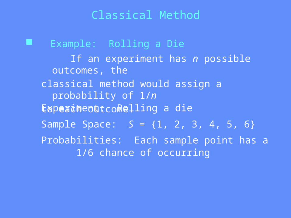
Classical Method
If an experiment has n possible outcomes, the
classical method would assign a probability of 1/n
to each outcome.Experiment: Rolling a die
Sample Space: S = {1, 2, 3, 4, 5, 6}
Probabilities: Each sample point has a 1/6 chance of occurring
Example: Rolling a Die

Relative Frequency Method
Number ofPolishers Rented
Numberof Days
01234
4 61810 2
Lucas Tool Rental would like to assign probabilitiesto the number of car polishers it rents each day. Office records show the following frequencies of dailyrentals for the last 40 days.
Example: Lucas Tool Rental
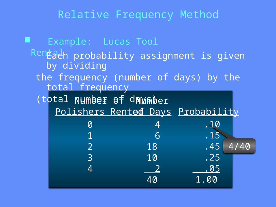
Each probability assignment is given by dividing
the frequency (number of days) by the total frequency
(total number of days).
Relative Frequency Method
4/40
ProbabilityNumber of
Polishers RentedNumberof Days
01234
4 61810 240
.10 .15 .45 .25 .051.00
Example: Lucas Tool Rental

Subjective Method
When economic conditions and a company’s circumstances change rapidly it might be inappropriate to assign probabilities based solely on historical data. We can use any data available as well as our experience and intuition, but ultimately a probability value should express our degree of belief that the experimental outcome will occur.
The best probability estimates often are obtained by combining the estimates from the classical or relative frequency approach with the subjective estimate.

Consider the case in which Tim and Judy Elsmore justmade an offer to purchase a house. Two outcomes arepossible:
E1 = their offer is accepted E2 = their offer is rejected
Judy believes the probability their offer will be accepted is 0.8; thus, Judy would set P(E1) = 0.8 and P(E2) = 0.2. Tim, however, believes the probability that their offer will be accepted is 0.6; hence, Tim would set P(E1) = 0.6 and P(E2) = 0.4. Tim’s probability estimate for E1 reflects a greater pessimism that their offer will be accepted.
Subjective Method
Example: House Offer
An event is a collection of sample points.
The probability of any event is equal to the sum of the probabilities of the sample points in the event.
If we can identify all the sample points of an experiment and assign a probability to each, we can compute the probability of an event.
Events and Their Probabilities

Events and Their Probabilities
Event E = Getting an even number when rolling a die
E = {2, 4, 6}
P(E) = P(2) + P(4) + P(6)= 1/6 + 1/6 + 1/6
= 3/6 = .5
Example: Rolling a Die
Some Basic Relationships of Probability
There are some basic probability relationships that
can be used to compute the probability of an event
without knowledge of all the sample point probabilities.
Complement of an Event
Conditional Probability
Multiplication Law
Addition Law

Bradley has invested in two stocks, Markley Oil
and Collins Mining. Bradley has determined that the
possible outcomes of these investments three months
from now are as follows. Investment Gain or Loss in 3 Months (in $000)
Markley Oil Collins Mining 10 5 0-20
8-2
Example: Bradley Investments
Some Basic Relationships of Probability
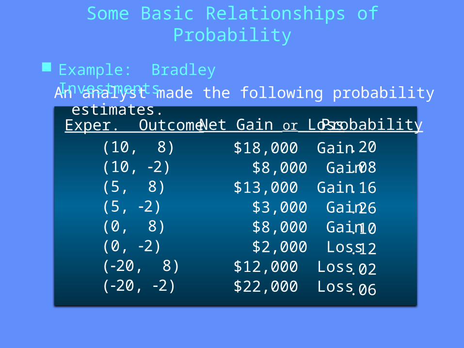
An analyst made the following probability estimates.
Exper. OutcomeNet Gain or Loss Probability(10, 8)(10, -2)(5, 8)(5, -2)(0, 8)(0, -2)(-20, 8)(-20, -2)
$18,000 Gain $8,000 Gain $13,000 Gain $3,000 Gain $8,000 Gain $2,000 Loss $12,000 Loss $22,000 Loss
.20
.08
.16
.26
.10
.12
.02
.06
Example: Bradley Investments
Some Basic Relationships of Probability
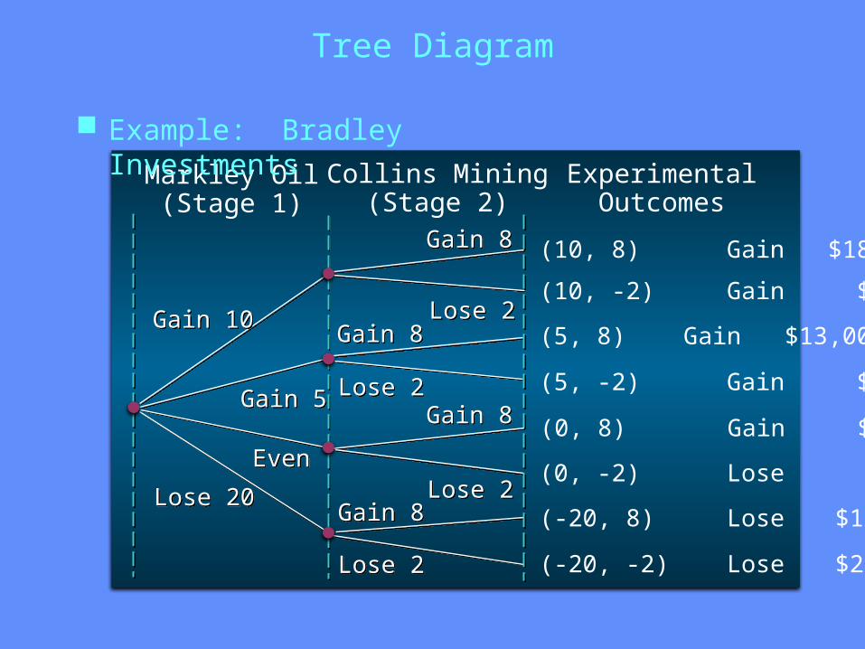
Tree Diagram
Gain 5Gain 5
Gain 8Gain 8
Gain 8Gain 8
Gain 10Gain 10
Gain 8Gain 8
Gain 8Gain 8
Lose 20Lose 20
Lose 2Lose 2
Lose 2Lose 2
Lose 2Lose 2
Lose 2Lose 2
EvenEven
Markley Oil(Stage 1)
Collins Mining(Stage 2)
ExperimentalOutcomes
(10, 8) Gain $18,000
(10, -2) Gain $8,000
(5, 8) Gain $13,000
(5, -2) Gain $3,000
(0, 8) Gain $8,000
(0, -2) Lose $2,000
(-20, 8) Lose $12,000
(-20, -2) Lose $22,000
Example: Bradley Investments
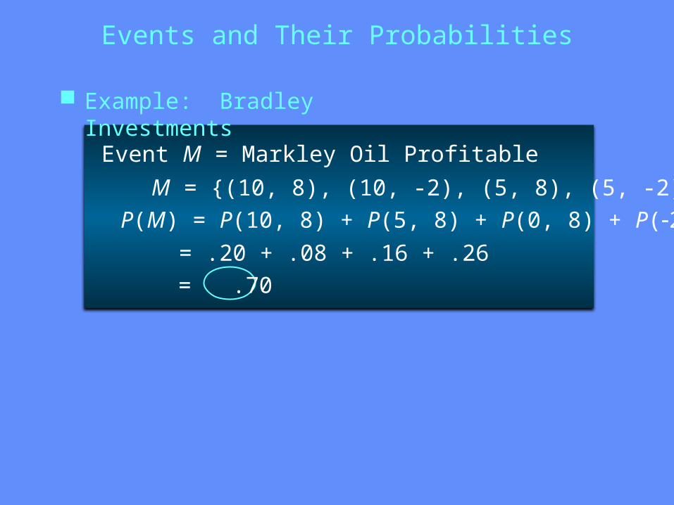
Events and Their Probabilities
Event M = Markley Oil Profitable
M = {(10, 8), (10, -2), (5, 8), (5, -2)}P(M) = P(10, 8) + P(5, 8) + P(0, 8) + P(-20, 8)
= .20 + .08 + .16 + .26= .70
Example: Bradley Investments

The complement of A is denoted by Ac.
The complement of event A is defined to be the event consisting of all sample points that are not in A.
Complement of an Event
Event A AcSampleSpace SSampleSpace S
VennDiagra
m
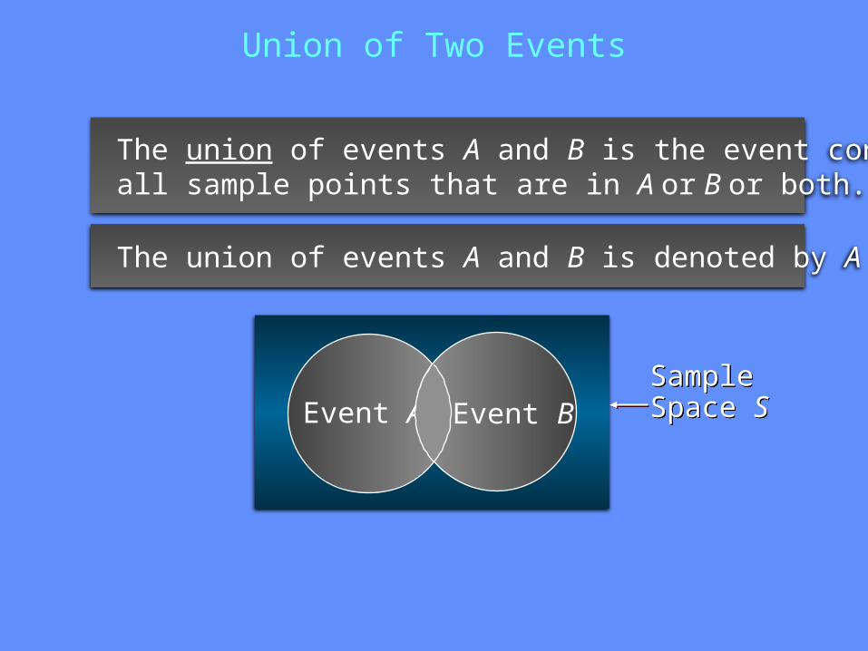
The union of events A and B is denoted by A B
The union of events A and B is the event containing all sample points that are in A or B or both.
Union of Two Events
SampleSpace SSampleSpace SEvent A Event B
Union of Two Events
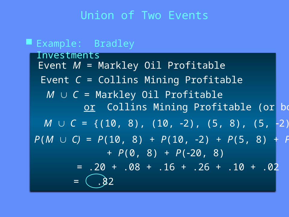
Event M = Markley Oil Profitable
Event C = Collins Mining Profitable
M C = Markley Oil Profitable or Collins Mining Profitable (or both)
M C = {(10, 8), (10, -2), (5, 8), (5, -2), (0, 8), (-20, 8)}
P(M C) = P(10, 8) + P(10, -2) + P(5, 8) + P(5, -2) + P(0, 8) + P(-20, 8)
= .20 + .08 + .16 + .26 + .10 + .02
= .82
Example: Bradley Investments
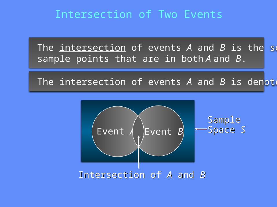
The intersection of events A and B is denoted by A
The intersection of events A and B is the set of all sample points that are in both A and B.
SampleSpace SSampleSpace SEvent A Event B
Intersection of Two Events
Intersection of A and BIntersection of A and B

Intersection of Two Events
Event M = Markley Oil Profitable
Event C = Collins Mining Profitable
M C = Markley Oil Profitable and Collins Mining Profitable
M C = {(10, 8), (5, 8)}
P(M C) = P(10, 8) + P(5, 8)
= .20 + .16
= .36
Example: Bradley Investments
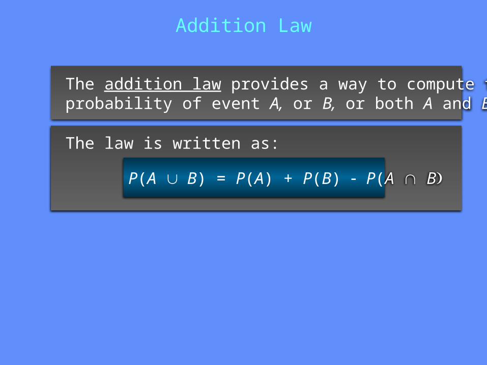
The addition law provides a way to compute the probability of event A, or B, or both A and B occurring.
Addition Law
The law is written as:
P(A B) = P(A) + P(B) - P(A B
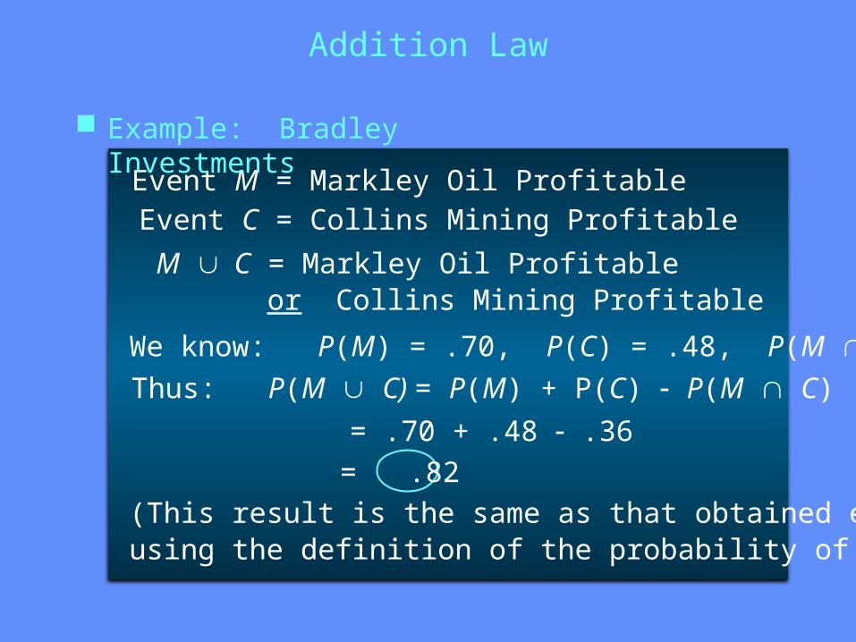
Event M = Markley Oil ProfitableEvent C = Collins Mining Profitable
M C = Markley Oil Profitable or Collins Mining Profitable
We know: P(M) = .70, P(C) = .48, P(M C) = .36
Thus: P(M C) = P(M) + P(C) - P(M C)
= .70 + .48 - .36= .82
Addition Law
(This result is the same as that obtained earlierusing the definition of the probability of an event.)
Example: Bradley Investments

Mutually Exclusive Events
Two events are said to be mutually exclusive if the events have no sample points in common.
Two events are mutually exclusive if, when one event occurs, the other cannot occur.
SampleSpace SSampleSpace SEvent A Event B

Mutually Exclusive Events
If events A and B are mutually exclusive, P(A B = 0.
The addition law for mutually exclusive events is:
P(A B) = P(A) + P(B)
There is no need toinclude “- P(A B”
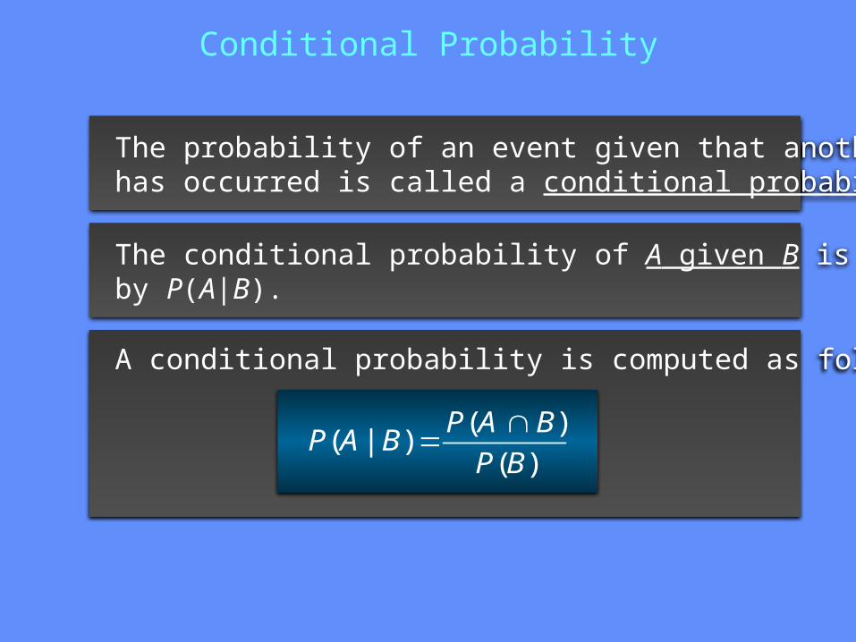
The probability of an event given that another event has occurred is called a conditional probability.
A conditional probability is computed as follows :
The conditional probability of A given B is denoted by P(A|B).
Conditional Probability
( )( | )
( )P A B
P A BP B

Event M = Markley Oil Profitable
Event C = Collins Mining Profitable
We know: P(M C) = .36, P(M) = .70
Thus:
Conditional Probability
( ) .36( | ) .5143
( ) .70P C M
P C MP M
= Collins Mining Profitable given Markley Oil Profitable
( | )P C M
Example: Bradley Investments

Multiplication Law
The multiplication law provides a way to compute the probability of the intersection of two events.
The law is written as:
P(A B) = P(B)P(A|B)

Event M = Markley Oil ProfitableEvent C = Collins Mining Profitable
We know: P(M) = .70, P(C|M) = .5143
Multiplication Law
M C = Markley Oil Profitable and Collins Mining Profitable
Thus: P(M C) = P(M)P(M|C)= (.70)(.5143)
= .36(This result is the same as that obtained earlierusing the definition of the probability of an event.)
Example: Bradley Investments

Joint Probability Table
Collins MiningProfitable (C) Not Profitable (Cc)Markley Oil
Profitable (M)
Not Profitable (Mc)
Total .48 .52
Total
.70
.30
1.00
.36 .34
.12 .18
Joint Probabilities(appear in the body
of the table) Marginal Probabilities(appear in the margins
of the table)
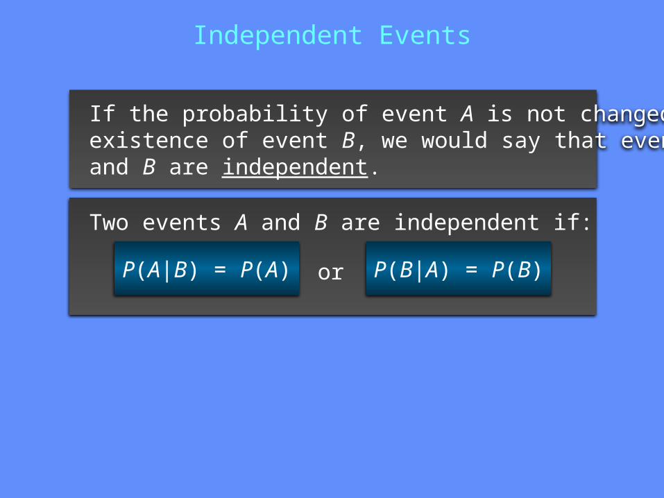
Independent Events
If the probability of event A is not changed by the existence of event B, we would say that events A and B are independent.
Two events A and B are independent if:
P(A|B) = P(A) P(B|A) = P(B)or

The multiplication law also can be used as a test to see if two events are independent.
The law is written as:
P(A B) = P(A)P(B)
Multiplication Lawfor Independent Events

Event M = Markley Oil ProfitableEvent C = Collins Mining Profitable
We know: P(M C) = .36, P(M) = .70, P(C) = .48 But: P(M)P(C) = (.70)(.48) = .34, not .36
Are events M and C independent?DoesP(M C) = P(M)P(C) ?
Hence: M and C are not independent.
Example: Bradley Investments
Multiplication Lawfor Independent Events

Do not confuse the notion of mutually exclusive events with that of independent events.
Two events with nonzero probabilities cannot be both mutually exclusive and independent.
If one mutually exclusive event is known to occur, the other cannot occur.; thus, the probability of the other event occurring is reduced to zero (and they are therefore dependent).
Mutual Exclusiveness and Independence
Two events that are not mutually exclusive, might or might not be independent.
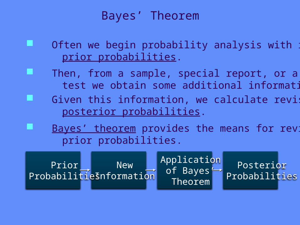
Bayes’ Theorem
NewInformation
Applicationof Bayes’Theorem
PosteriorProbabilities
PriorProbabilities
Often we begin probability analysis with initial or prior probabilities.
Then, from a sample, special report, or a product test we obtain some additional information. Given this information, we calculate revised or posterior probabilities.
Bayes’ theorem provides the means for revising the prior probabilities.
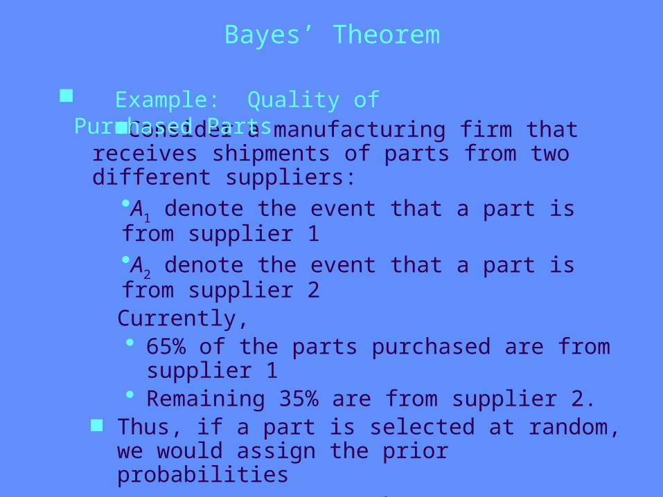
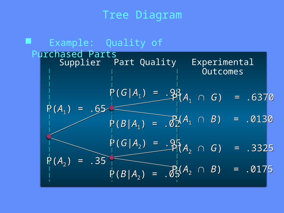
Consider a manufacturing firm that receives shipments of parts from two different suppliers:
•A1 denote the event that a part is from supplier 1 •A2 denote the event that a part is from supplier 2 Currently, • 65% of the parts purchased are from
supplier 1• Remaining 35% are from supplier 2.
Thus, if a part is selected at random, we would assign the prior probabilities
P(A1) = 0.65 and P(A2) = 0.35.
Bayes’ Theorem
Example: Quality of Purchased Parts

The quality of the purchased parts varies with the
source of supply. Let • G denote the event that a part is good• B denote the event that a part is bad.
Based on historical data, the conditional probabilities
of receiving good and bad parts from the two suppliers are:
P(G | Al) = 0.98 and P(B | A1) = 0.02
P(G | A2) = 0.95 and P(B | A2) = 0.05
Bayes’ Theorem
Example: Quality of Purchased Parts
P(B|A1) = .02P(B|A1) = .02
P(A1) = .65P(A1) = .65
P(A2) = .35P(A2) = .35
P(G|A2) = .95P(G|A2) = .95
P(B|A2) = .05P(B|A2) = .05
P(G|A1) = .98P(G|A1) = .98 P(A1 G) = .6370P(A1 G) = .6370
P(A2 G) = .3325P(A2 G) = .3325
P(A2 B) = .0175P(A2 B) = .0175
P(A1 B) = .0130P(A1 B) = .0130
Supplier Part Quality ExperimentalOutcomes
Tree Diagram
Example: Quality of Purchased Parts

A bad part caused one machine to break down.What is the probability that the bad part came from supplier 1What is the probability that it came from supplier 2?
With the information in the probability tree, we
can use Bayes’ theorem to answer these questions.
New Information
Example: Quality of Purchased Parts
Bayes’ Theorem
1 1 2 2
( ) ( | )( | )
( ) ( | ) ( ) ( | ) ... ( ) ( | )i i
in n
P A P B AP A B
P A P B A P A P B A P A P B A
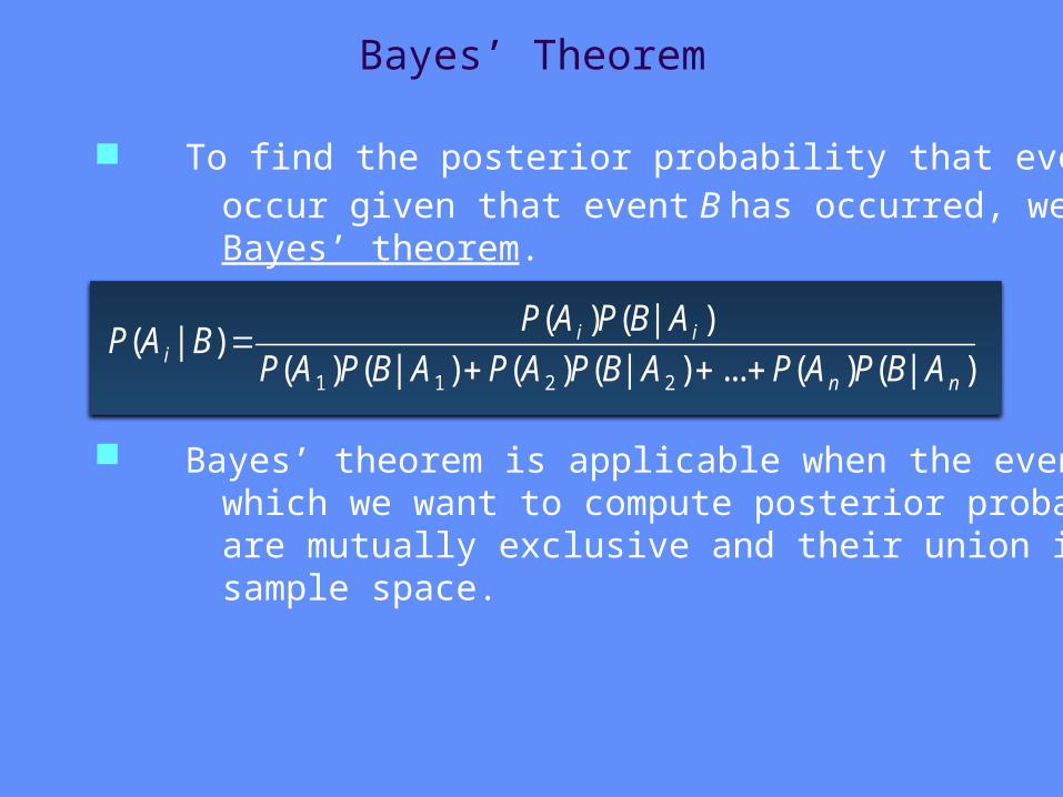
To find the posterior probability that event Ai will occur given that event B has occurred, we apply Bayes’ theorem.
Bayes’ theorem is applicable when the events for which we want to compute posterior probabilities are mutually exclusive and their union is the entire sample space.

Given that the part received was bad, we revise
the prior probabilities as follows:
1 11
1 1 2 2
( ) ( | )( | )
( ) ( | ) ( ) ( | )P A P B A
P A BP A P B A P A P B A
(.65)(.02)(.65)(.02) (.35)(.05)
Posterior Probabilities
= .4262
Example: Quality of Purchased Parts

Bayes’ Theorem: Tabular Approach
Example: Quality of Purchased Parts
Column 1 - The mutually exclusive events for which posterior probabilities are desired.
Column 2 - The prior probabilities for the events.
Column 3 - The conditional probabilities of the new information given each event.
Prepare the following three columns:• Step 1

(1) (2) (3) (4) (5)
Events
Ai
PriorProbabilities
P(Ai)
ConditionalProbabilities
P(B|Ai)
A1
A2
.65
.35
1.00
.02
.05
Example: Quality of Purchased Parts
Bayes’ Theorem: Tabular Approach
• Step 1
Bayes’ Theorem: Tabular Approach
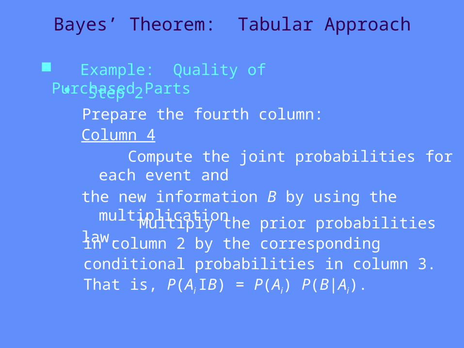
Column 4 Compute the joint probabilities for each event
andthe new information B by using the multiplicationlaw.
Prepare the fourth column:
Multiply the prior probabilities in column 2 by the corresponding conditional probabilities in column 3. That is, P(Ai IB) = P(Ai) P(B|Ai).
Example: Quality of Purchased Parts• Step 2

(1) (2) (3) (4) (5)
Events
Ai
PriorProbabilities
P(Ai)
ConditionalProbabilities
P(B|Ai)
A1
A2
.65
.35
1.00
.02
.05
.0130
.0175
JointProbabilities
P(Ai I B)
.65 x .02
Example: Quality of Purchased Parts
Bayes’ Theorem: Tabular Approach
• Step 2
• Step 2 (continued)
We see that there is a .0130 probability of thepart coming from supplier 1 and the part is bad.
Example: Quality of Purchased Parts
Bayes’ Theorem: Tabular Approach
We see that there is a .0175 probability of thepart coming from supplier 2 and the part is bad.

• Step 3
Sum the joint probabilities in Column 4. Thesum is the probability of the new information,P(B). The sum .0130 + .0175 shows an overallprobability of .0305 of a bad part being received.
Example: Quality of Purchased Parts
Bayes’ Theorem: Tabular Approach

(1) (2) (3) (4) (5)
Events
Ai
PriorProbabilities
P(Ai)
ConditionalProbabilities
P(B|Ai)
A1
A2
.65
.35
1.00
.02
.05
.0130
.0175
JointProbabilities
P(Ai I B)
P(B) = .0305
Example: Quality of Purchased Parts
Bayes’ Theorem: Tabular Approach
• Step 3
( )( | )
( )i
i
P A BP A B
P B
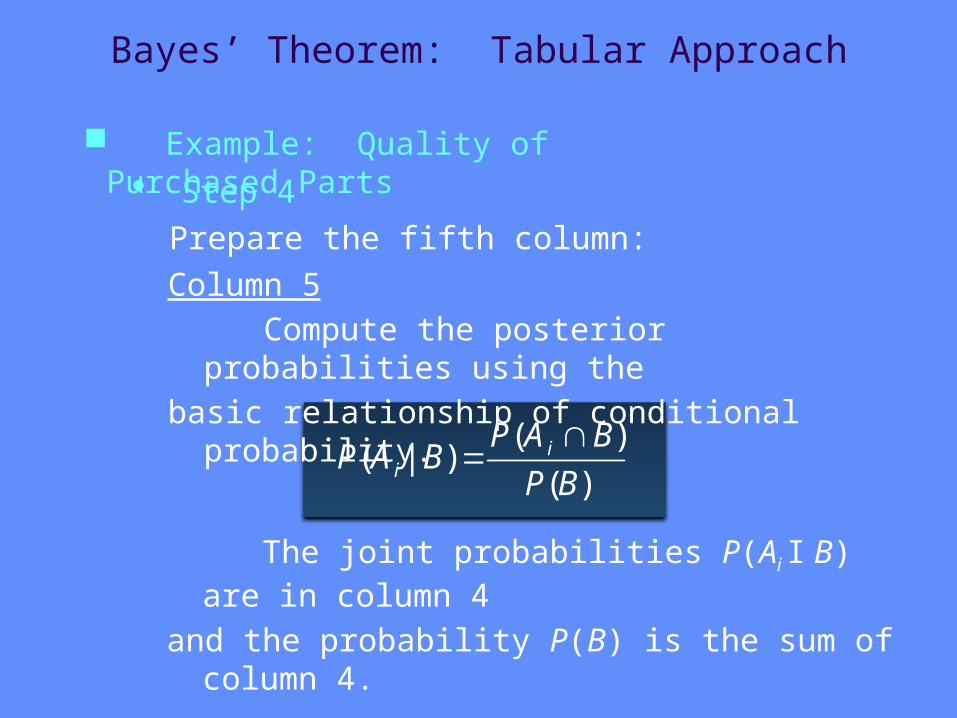
Bayes’ Theorem: Tabular Approach
Prepare the fifth column:
Column 5 Compute the posterior probabilities using
thebasic relationship of conditional probability.
Example: Quality of Purchased Parts• Step 4
The joint probabilities P(Ai I B) are in column 4
and the probability P(B) is the sum of column 4.

(1) (2) (3) (4) (5)
Events
Ai
PriorProbabilities
P(Ai)
ConditionalProbabilities
P(B|Ai)
A1
A2
.65
.35
1.00
.02
.05
.0130
.0175
JointProbabilities
P(Ai I B)
P(B) = .0305.0130/.0305
PosteriorProbabilities
P(Ai |B)
.4262
.5738
1.0000
Example: Quality of Purchased Parts
Bayes’ Theorem: Tabular Approach
• Step 4

Crosstabulation: Simpson’s Paradox
In some cases the conclusions based upon an aggregated crosstabulation can be completely reversed if we look at the disaggregated data. The reversal of conclusions based on aggregate and disaggregated data is called Simpson’s paradox.
We must be careful in drawing conclusions about the relationship between the two variables in the aggregated crosstabulation.
Data in two or more crosstabulations are often aggregated to produce a summary crosstabulation.

Chapters Making Use of Probability
Chapter 3 – Probability Distributions
Chapter 5 – Utility and Game Theory Chapter 13 – Project Scheduling: PERT/CPM Chapter 14 – Inventory Models
Chapter 4 – Decision Analysis
Chapter 15 – Waiting Line Models
Chapter 16 - Simulation
Chapter 17 – Markov Processes


