CHAPTER 2 LIMITS Limits provide the foundation for all the key ideas of calculus (differentiation, integration, and infinite series, to name a few). This chapter supplies the tools that your students will use to understand the important concepts of calculus.
2.1 The Idea of Limits
Overview
In this opening section, we introduce the idea of a limit through an investigation of the relationship between instantaneous velocity and tangent lines. The intent is to provide students with motivation for the entire chapter and to give an intuitive sense of how limits work. We feel this material is essential even though tangent lines and instantaneous velocity are treated in more detail in Chapter 3.
Lecture Support Notes
Limits arise naturally when we define instantaneous velocity and the line tangent to a curve.
• Ask students to compute an average velocity for a simple situation (e.g. a car travels 110 mi in 2 hr;
what is its average velocity?). Increase the complexity of the problem by providing a plausible position function for an object, and ask students to compute the average velocity over some time interval. Students should be able to come up with the formula
average velocity = (change in position)/(change in time). • Point out that average velocities are just slopes of secant lines on a position curve (Example 1; Figures
2.1–2.3). • Show how average velocity can be used to approximate instantaneous velocity. • Then show how shrinking the time interval leads to better approximations of instantaneous velocity. • Introduce the idea of a limit in moving from average to instantaneous velocity (Example 2).
This scheme can be repeated to introduce the notion of a tangent line as the limit of approaching secant lines. Students can compute the slopes of secant lines over smaller intervals to arrive at a preliminary definition for the slope of a tangent line. Emphasize ideas rather than details; the details will come in later sections. Interactive Figures
• Figures 2.1–2.2 display the position and average velocity of a rock for 0 3.t≤ ≤ • Figure 2.4 illustrates calculating instantaneous velocity via limits. • Figure 2.5–2.6 display the tangent and secant lines, while the latter also displays average and
This section lays the foundation for a formal discussion of tangent lines and instantaneous velocity found in Chapter 3. Examples 1 and 3 of Section 3.1 build upon the ideas introduced in Examples 1 and 2 of Section 2.1.
• Section 1.2 includes a review of linear functions and the formula for the slope of a line through two
points. • Section 3.5 continues the discussion of the derivative as a rate of change (instantaneous velocity in
particular). • Remind students to bring calculators or laptops to the next class if you intend to call upon them to
produce the graphs and tables necessary to determine limits.
Additional Activities
Suggested Guided Project: Local Linearity is a guided project that fits well with this section; it extends the idea introduced in the margin note on page 35 of the text. Part 1 of this project could be used in class as a launching point for a discussion about tangent lines (the remainder could be assigned for completion outside of class.)
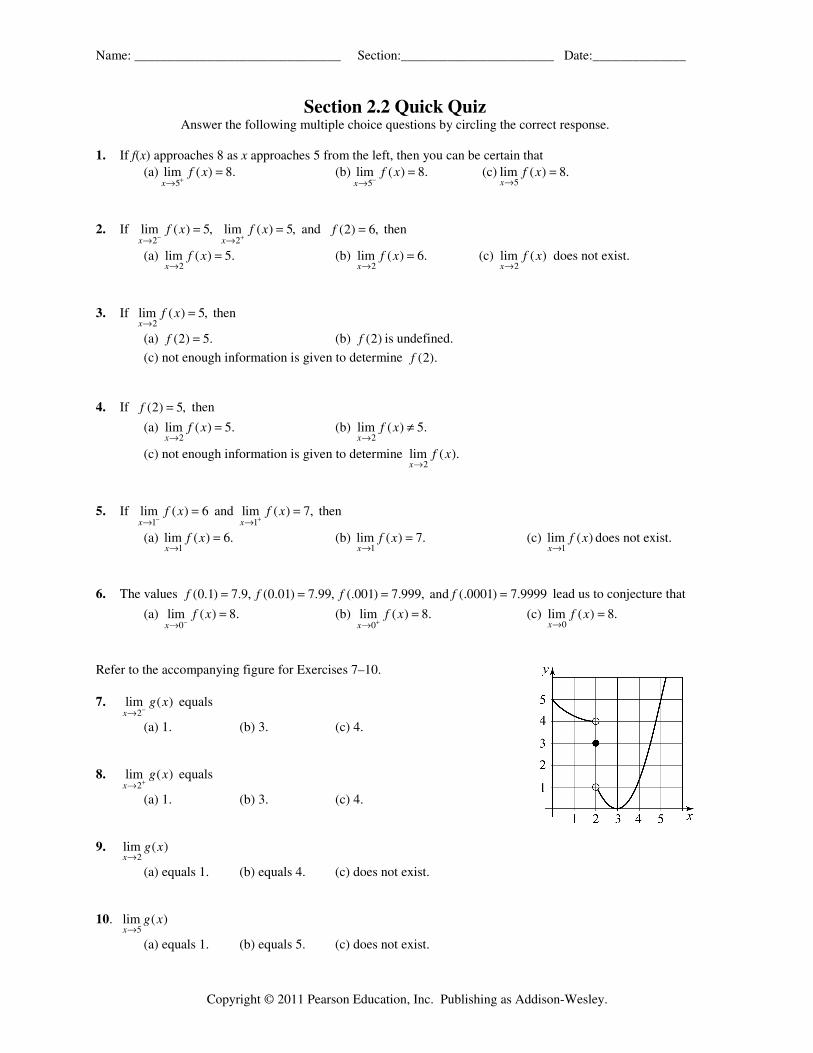
This section gives a standard treatment of left-hand, right-hand, and two-sided limits, and shows how to compute them (informally) with graphs and numerical methods.
Lecture Support Notes
A preliminary (informal) definition of a limit is adequate for understanding and computing most of the limits encountered in the text.
• Present the informal definition of a limit. • At this stage, computing the value of a limit is most easily carried out with a graph (Example 1). Point
out that the limit of a function f at the point a (if it exists) does not depend upon the value of ( )f a .
• The value of a limit at a point can also be investigated by tabulating function values near that point
(Example 2). • Introduce left- and right-hand limits (Example 3) and their relationship to the corresponding two-sided
limit. • Show that limits may fail to exist, either because the left- and right-hand limits do not agree (Example
4), or because the values of a function do not approach a single number (Example 5).
Interactive Figures
• Figures 2.7–2.10 illustrate how to find a limit of a function. • Figure 2.11 illustrates how computer generated plots often do not plot where the function is undefined. • Figure 2.12 displays limits from the left and right. • Figure 2.14 zooms in on ( )cos 1/y x= near 0.x =
Connections
Most of the exercises in this section rely upon a graph or a table. For those exercises where students must produce a graph, we expect them to rely on technology at this point in the course—be prepared to help with various calculators and software packages. That said, students should begin the work of mastering the basic graphs of all the familiar functions (presented in Sections 1.2–1.3).
Cover Example 3 (or use a function similar to Exercise 15 as a suitable replacement with easier factoring) for an easy-to-implement, in-class activity. Assign various values of x in Table 2.3 to rows of students in your classroom, and ask them to compute f(x) on a calculator. Solicit responses from each row and fill in a table at the board, from which the class can determine the limit. This is just the preliminary work for the intended activity: Explore the algebraic reasons behind the value of the limit (alluding to techniques introduced in
Section 2.3) by showing that 3 28 2 4
4( 2) 4
x x x
x
− + +=−
( 2x ≠ ). The graph of the function on the right side of the
equation is the parabola 2 314 4( 1)y x= + + . Ask students to verify that the graph of the function on the left side
of the equation has the same graph except at 2x = , and that the values of 2 314 4( 1)y x= + + approach 3 as x
approaches 2. With this activity, you can review factoring formulas (difference of perfect cubes), completing the square, the standard form of a parabola ( 2( )y a x h k= − + , whose vertex is ( , )h k ), and graphing parabolas
Analytical methods for evaluating limits are presented.
Lecture Support Notes
Limits of polynomial, rational, and algebraic functions can usually be evaluated by direct substitution, provided the function is defined at the limit point (exceptions include piecewise functions; see Example 5). Limit laws, algebraic manipulation, and the Squeeze Theorem provide tools for evaluating more challenging limits.
• Pack in as many examples as class time allows, using graphs to illustrate the fact that lim ( ) ( )
x af x f a
→=
for many standard functions. At this point we have neither the tools nor the concepts—namely, the -ε δ definition of a limit and continuity—to prove Theorems 2.2–2.4 rigorously, so it is important to
provide visual evidence that these theorems are true. • Limits that cannot be evaluated by direct substitution can often be transformed into limits that yield to
direct substitution via factoring and multiplication by the conjugate. In some cases, the Squeeze Theorem is an essential tool.
• Consider beginning the task of identifying standard limit forms in this section. For instance, you could
point out that the limits in Example 6 are of the form 0/0, one of several indeterminate forms to be treated in Section 4.7. Students will have an easier time deciding which technique to apply to a particular limit if they can identify the form of a limit.
• Cover Example 7 if you intend to offer (in Section 2.6) a rigorous proof that the sine and cosine
functions are continuous on their domains.
Interactive Figures
• Figure 2.15 displays limits and slopes of the tangent line from the left and from the right. • Figure 2.19 illustrates the squeeze theorem. Figures 2.20–2.21 illustrate the squeeze theorem for
particular trigonometric functions.
Connections
• Example 7 is needed to show that the sine and cosine functions are continuous on their domains. • The justification for the method of direct substitution, continuity, is presented in Section 2.6.
This is the first section in our study of calculus where students will be required to draw fully on their knowledge of algebra (in particular, factoring polynomials, simplifying rational functions, and using the technique of multiplying by a conjugate). The following selection of exercises can be used as a “math minute” activity, where students have one minute (or longer if you so choose) to complete as many problems as possible. Five minutes is a more reasonable amount of time if you expect students to complete all of the problems.
To motivate your students, point out that these drill problems are linked directly to the exercise set (Exercises 37–40, 42–45, and 58–60). If they can get through these quickly, evaluating the limits that are associated with them won’t seem so bad. Provide answers at the end of the activity so that students can assess whether they need more practice (given the pressures associated with completing the problems at a fast pace, this exercise is not intended to count toward a student’s grade; rather, it’s meant to be a fun way to engage your students and help them identify their weak areas). If you have not already done so, this would be a good time in the semester to advertise the resources available to students at MyMathLab.
Infinite limits are introduced (initially alongside a limit at infinity to help students distinguish between the two scenarios), and their connection to vertical asymptotes is explained.
Lecture Support Notes
• Make the distinction between infinite limits and limits at infinity so that students understand their
similarities and differences before moving onto Section 2.5. • It is important that students understand that an infinite limit does not exist; we only use the symbol ∞
as a convenience to indicate that the function attains arbitrarily large values. It doesn’t hurt to explain this once more after one-sided infinite limits are introduced: We say a two-sided limit is ∞ (or −∞ ) only when the left- and right-hand limits “agree,” despite the fact that neither the left nor right-hand limit exists.
• The graph of f has the vertical asymptote x a= whenever the limit of f (left, right, or two-sided) is
infinite in magnitude at a. • Consider employing the notation “ / 0L + ” and “ / 0L − ” (where L is a nonzero constant) for those limits
where the numerator approaches L and the denominator approaches 0, either from above or below. This notation sees widespread use, and certainly has value—the authors decided against formally introducing it in the text for various reasons. If you spend the time in class to develop and explain the notation, it gives students another tool for getting an intuitive feel for the value of a limit. Example 5 provides a good illustration of the different behaviors that can arise when the denominator of a function approaches 0.
Interactive Figures
• The figures accompanying Tables 2.5–2.6 illustrate infinite limits. • Figure 2.27 illustrates how computer generated plots often do not include undefined points and make
vertical asymptotes appear as a solid line (rather than the dotted line that is seen in the text).
Connections
• Vertical asymptotes make a brief appearance in Chapter 1 (Section 1.2 and Section 1.3 in connection
with trigonometric functions). They are also treated in Section 4.3 in conjunction with graphing functions.
• Vertical tangent lines are later discussed on pp. 108–9; see also Exercises 61–64 in Section 3.1.
Chapter 2 opens with a brief discussion of tangent lines; the tangent problem is then set aside for most of the remainder of the chapter. (We pick it up again in Chapter 3.) If you’d like to continue to develop tangent lines alongside the discussion of limits, here’s an activity that incorporates infinite limits and vertical tangent lines. The idea is to find the slope of the line tangent to the unit circle at (1,0) and ( 1,0)− .
• Let 2( , 1 )P x x− denote a variable point on the upper half of the unit circle, with 0 1x≤ < . The slope
of the secant line between P and (1,0) is 2
sec
1
1
xm
x
−=
−.
• The slope of the tangent line at (1,0) is 2
tan1
1lim
1x
xm
x−→
−=
−.
• This limit can be investigated numerically by choosing values of 1x < that get closer to 1, and/or by
algebraic manipulation: 2
tan1 1 1
1 1 1 1lim lim lim
1 (1 ) 1x x x
x x x xm
x x x− − −→ → →
− − + += = = −− − − −
,
where the limit on the right is of the form 2 / 0+− = −∞ . • Interpret this limit to show that the graph of the unit circle has a vertical tangent line at (1,0) .
• A similar argument shows that the unit circle also has a vertical tangent line at ( 1,0)− , though the limit
in this case is ∞ (assuming as before that P is a point on the upper half of the unit circle). This activity could be teacher-directed (walk through the above steps with your students, supplying additional details where necessary), or modified to be given as an out of class project. One could also analyze the minor
differences that appear when the point P is selected on the lower half of the circle. Note that 2
1
1lim
1x
x
x−→
−−
is of
the form 0/0: If you introduced this notation to your class in earlier sections (e.g. Example 6 in Section 2.3), this activity helps to drive home the reason why we label “0/0” as an indeterminate form. Though students aren’t quite ready to hear it (because we have not yet introduced the derivative), it’s worth noting the difference between the limits investigated in this activity and the more standard limits of this section. After derivatives have been covered, come back to this activity and point out that when lim ( )
x af x
+→= ±∞′ (or lim ( )
x af x
−→′ = ±∞ ),
there is a vertical tangent at x a= (assuming that a is in the domain of f ). When lim ( )x a
f x+→
= ±∞ , we
conclude that the graph of f has a vertical asymptote at x a= .
Limits at infinity determine the end behavior of a function, detect the presence of horizontal asymptotes, and reveal whether a system attains a steady state.
Lecture Support Notes
• When they exist, limits at infinity indicate a horizontal asymptote. • As with Section 2.4, it’s worth pointing out that infinite limits at infinity do not exist; contrast this
situation with lim cosx
x→∞
, which also does not exist, but for different reasons.
• Include examples from all the standard families of functions so that students get a feel for the end
behavior of the various functions they will encounter throughout the text. Theorems 2.6 and 2.7 are particularly important as they allow students to quickly evaluate many limits at infinity.
• Be cautious with slant asymptotes. For instance, in Example 3c, it’s easy for students to apply this
faulty logic:
22
2 62 6 2lim lim lim(2 6)
11 1x x x
xx x x xx
x
→∞ →∞ →∞
+ −+ − = = ++ +
,
which implies that 2 6y x= + and 22 6 2
( )1
x xh x
x
+ −=
+ behave the same way as x gets large, and
therefore 2 6y x= + is an asymptote for the graph of h (this is incorrect). The proper method for
finding a slant asymptote is to perform long division. • This section offers another opportunity to include informal notation for limits that can be very useful
for students. For example, limits where the numerator approaches any constant L and where the denominator approaches ±∞ can be labeled “ /L ∞ ,” the value of which is 0. The indeterminate form
/∞ ∞ also makes an appearance in this section; we leave it to you to decide whether to draw attention to this form at this point in the course.
Interactive Figures
• Figures 2.30–2.32 illustrate horizontal asymptotes. • Figures 2.33–2.34 illustrate infinite limits as x approaches infinity. • Figures 2.35–2.37 illustrate the behavior of rational functions as x approaches infinity. • Figure 2.38 illustrates the behavior of an algebraic function as x approaches infinity.
• Horizontal asymptotes are briefly mentioned in Section 1.2. • It may be helpful to introduce notation that will be used later in the text (Section 4.7, L’Hôpital’s
Rule); there are ample opportunities in this section to point out the indeterminate form /∞ ∞ . • The absolute value function (and its piecewise definition) is covered in Section 1.2; the subtleties of
Example 4 require a good understanding of x .
Additional Activities
Guided Project: Fixed Point Iteration explores the idea of the limit of a sequence. It provides (and asks for) illustrations of a limit at infinity in the context of solving equations, and is particularly well suited to visual learners. Here is another math minute activity that is intended for use after students have mastered the material in this section and Section 2.4. If you introduced the notations / 0L ± , /L ∞ , and /∞ ∞ , encourage students to identify the form of each limit before coming to an answer.
A standard treatment of continuity is offered, with the important Intermediate Value Theorem given at the end of the section.
Lecture Support Notes
The authors made a conscious decision to avoid defining the phrase “continuous function,” which is usually taken to mean a function continuous on its domain. Rather, we are careful to claim that a function is continuous either at a point, or on an interval (occasionally specified only as the domain of the function in question, which of course could be a collection of intervals). The reason behind this decision: It is correct to say that
( ) 1/f x x= is a continuous function, and yet it has a discontinuity at 0x = . Avoiding this apparent
inconsistency in terminology is easier on students who are encountering continuity for the first time. • Show that the definition of continuity allows the use of direct substitution when evaluating lim ( )
x af x
→,
provided f is continuous at a. • Figure 2.40 (and its corresponding function) is useful to illustrate why we need a precise definition for
continuity. • Establish the fact that all the standard families of functions (polynomial, rational, trigonometric, etc.)
are continuous on their domains. • Cover Theorem 2.10; it is used to evaluate limits of the composition of functions.
Interactive Figures
• Figure 2.40 zooms in on a piecewise function to illustrate continuity at a point. • Figure 2.43 illustrates left-continuity and right-continuity. • Figure 2.44 illustrates intervals of continuity. • Figure 2.45 illustrates continuity near roots. • Figures 2.48–2.49 illustrate the Intermediate Value Theorem.
Connections
• The Intermediate Value Theorem is used in subsequent sections to prove additional results (e.g. the
Mean Value Theorem for Integrals in Section 5.4). • The property of continuity is the justification for the method of substitution used in previous sections
The Intermediate Value Theorem can be used to zero in on a root of an equation using the bisection method. For example, consider the function ( ) xf x e x= + , which is continuous on ( , )−∞ ∞ . Because ( 1) 0f − < , and
(0) 0f > , we know ( ) 0f x = has at least one solution on [ 1,0]− , though we can’t solve the equation using
standard techniques from algebra. A graph of the function shows that there is only one solution on [ 1,0]− (this
fact can be proved by noting that ( ) 0f x >′ on [ 1,0]− —in fact, on ( , )−∞ ∞ —but students aren’t ready for this
argument at the moment, and therefore a graph is the best we can do). One strategy for finding the root is to evaluate f with a calculator at the midpoint of [ 1,0]− , and then use that information to determine a new interval
on which ( ) 0f x = is guaranteed to have a solution. Because ( 0.5) 0f − > , we know that the solution lies in
[ 1, 0.5]− − . Continuing in this manner, the solution can be determined up to the accuracy of the calculating
device used, albeit with a great deal of tedium. A better approach is to discuss with your students how the strategy might be implemented, and then to carry it out by writing a program (on a TI-83, using Excel, Mathematica, or whatever technology you prefer).
The following table can be used to find the root of ( ) 0f x = using an Excel spreadsheet. If you intend
for your students to understand the algorithm, you will need to explain how the Excel function IF behaves (alternatively, you could explain that you’ve created the code necessary to carry out the bisection method). Select cells A3 through E3, drag your mouse down to highlight as many rows as you like, and then choose Edit > Fill > Down (we assume some familiarity with Excel; it doesn’t take much to learn it well enough to include this activity in class).
A B C D E
1 Left endpoint Right endpoint New midpoint f(left endpoint) f(right endpoint) 2 -1 0 =(A2+B2)/2 =EXP(A2)+A2 =EXP(B2)+B2 3 =IF((EXP(C2)+
C2)>0,A2,C2) =IF((EXP(C2)+C2)>0,C2,B2)
=(A3+B3)/2 =EXP(A3)+A3 =EXP(B3)+B3
The values in columns A and B converge to the root of ( ) 0f x = . Columns D and E aren’t entirely necessary,
though they provide a check on whether the values of f at the endpoints are as they should be with regard to sign and value (column D should contain negative values, column E positive values, and both should appear to converge to 0).
If you don’t want to introduce the exponential function at this stage in the semester, the next spreadsheet solves ( ) cos 0g x x x= − = on the interval [0,1] . It assumes we already know (0) 0g > and
(1) 0g < , and that there is only one solution on this interval (this can be proved by looking at ( )g x′ , or by
showing students a graph).
A B C D E 1 Left endpoint Right endpoint New midpoint g(left endpoint) g(right endpoint) 2 0 1 =(A2+B2)/2 =COS(A2)-A2 =COS(B2)-B2 3 =IF((COS(C2)-
C2)>0,C2,A2) =IF((COS(C2)-C2)>0,B2,C2)
=(A3+B3)/2 =COS(A3)-A3 =COS(B3)-B3
Notice the subtle difference between the formula in cell A3 given here, and the formula in cell A3 from the preceding example: In the IF statement, the order of C2 and A2 has been switched (this transposition also occurs in cell B3). This is necessary because f is increasing on [0,1] , whereas g is decreasing on [0,1] . These
facts affect how the new endpoints should be chosen for the next step. These two examples alone provide ample material for students to wrestle with, particularly if you ask
them to create a spreadsheet (or write a program) on their own.
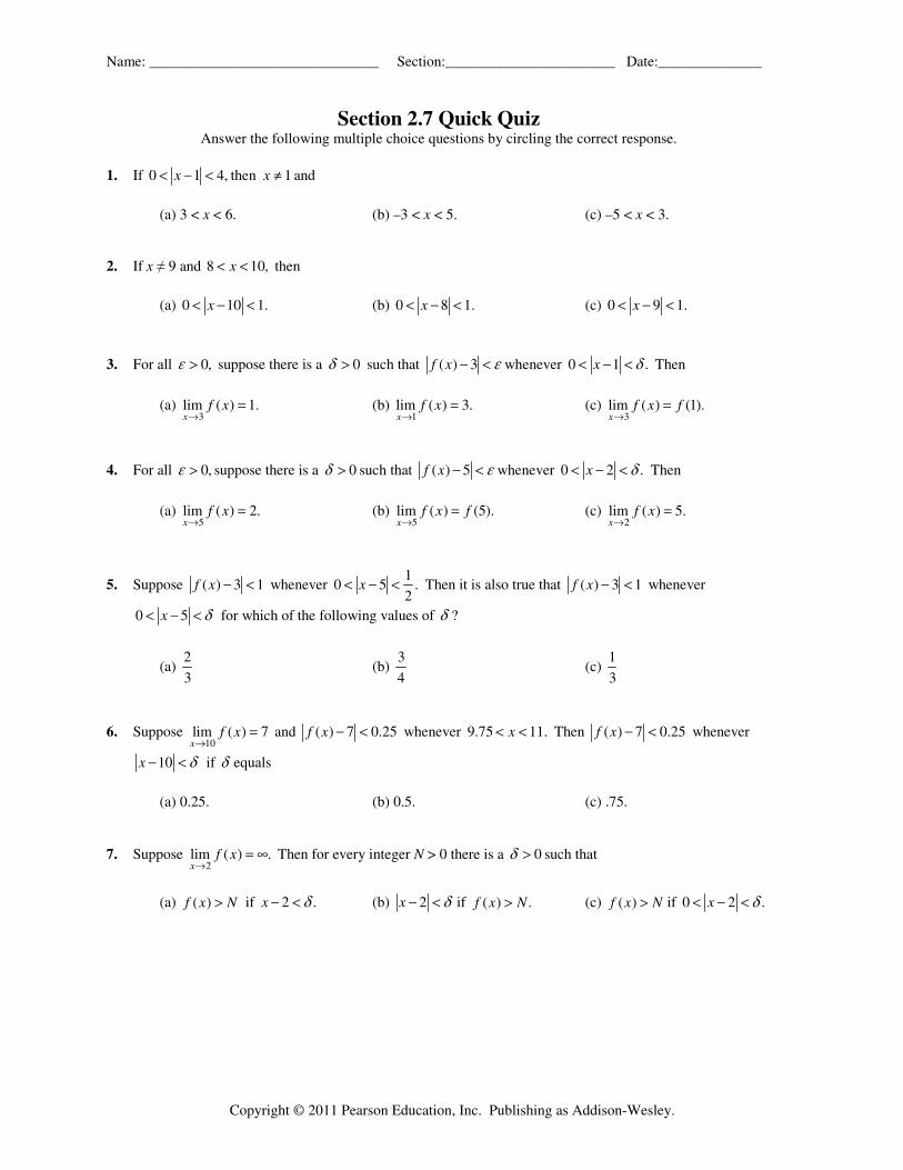
The -ε δ definition of a limit is presented, allowing rigorous proofs of limits and limit laws.
Lecture Support Notes
This optional section is challenging for students. Depending on your students, you might want to keep the technical details to a minimum by focusing on limits of linear functions or piecewise linear functions (Examples 1, 3, and 4 provide a nice progression from the idea of a rigorous limit to the proof of a limit). Once students grasp the concept of a limit proof, prove at least one of the limit laws (Example 5). Assigning Exercise 28 helps to put the concept of continuity on a solid foundation.
Interactive Figures
• Figures 2.52–2.54 introduce how and δ ε relate in moving toward a precise definition of the limit. • Figure 2.55 illustrates how and δ ε relate in the precise definition of the limit. • Figures 2.59–2.60 illustrate how to find symmetric intervals. • Figure 2.61 illustrates the precise definition of an infinite limit.
Connections
If you intend to introduce more formality into the idea of a limit later in the calculus curriculum (e.g. Sections 9.2 and 13.3), it may be worth covering at least the basic ideas of this section.
Additional Activities
If you want to add more material to this section, Exercises 50–53 deal with limits at infinity (both finite and
infinite). Using the definition given in Exercises 50–51, discuss the proof of 1
lim 1x
x
x→∞
+= (choose 1/N ε= )
with your students to prepare them for the exercises in the text.
18–19. Determining infinite limits analytically Determine the following limits, if possible.
18. 5
6lim
5x
x
x−→
−−
19. 2
2
2lim
2x
x x
x+→−
+ −+
20–21. Horizontal asymptotes Evaluate lim ( )x
f x→∞
and lim ( )x
f x→−∞
. State the horizontal asymptote(s) of f .
20. 9
10
6000 9 8( )
6 2
x xf x
x x
− +=− +
21. 5 3
10 8 4
16 13 1( )
64 10 2
x xf x
x x x
+ +=+ +
22–23. Horizontal and Vertical Asymptotes
a. Find the horizontal and vertical asymptotes of the following functions. Evaluate the appropriate limits to justify your answers.
b. Use a graphing utility to graph the function. Then sketch a graph of the function by hand, correcting any errors appearing in the computer-generated graph.
22. 2
4( )
1
xf x
x=
+ 23.
2
3
3( )
3 5 8
x xf x
x x
+=+ −
24–25. Determining continuity at a point Determine whether the following functions are continuous at x a= using the Continuity Check List to justify your answer.
24.
2 1if 1
( ) ; 112 if 1
xx
f x axx
⎧ −⎪ ≠= =⎨ −⎪ =⎩
25.
2 4 3if 3
( ) ; 332 if 3
x xx
f x axx
⎧ − +⎪ ≠= =⎨ −⎪ =⎩
26. Determining an unknown constant Determine the value of the constant a for which the function
2 5 2 if 1( )
3 if 1
x x xg x
x a x
⎧ + + ≤⎪= ⎨+ >⎪⎩
is continuous at 1x = .
27. Determining unknown constants Let
2 2 if 1
( ) 3 if 1
2 if 1
x x a x
g x x
bx x
⎧ − + <⎪
= =⎨⎪ + >⎩
.
a. Determine values of a and b for which g is continuous at 1x = .
b. For what values of a and b is g continuous from the left at 1x = , but not continuous from the right at
1x = ?
c. For what values of a and b is g continuous from the right at 1x = , but not continuous from the left at