CHAPTER 2 Matrices - testbanklive.com · Section 2.4 Elementary Matrices ... Project Solutions ......

© 2017 Cengage Learning. All Rights Reserved. May not be scanned, copied or duplicated, or posted to a publicly accessible website, in whole or in part.

C H A P T E R 2 Matrices

Section 2.1 Operations with Matrices ..................................................................... 30

Section 2.2 Properties of Matrix Operations ........................................................... 36

Section 2.3 The Inverse of a Matrix ........................................................................ 41

Section 2.4 Elementary Matrices ............................................................................. 46

Section 2.5 Markov Chains ..................................................................................... 53

Section 2.6 More Applications of Matrix Operations ............................................ 62

Review Exercises .......................................................................................................... 66

Project Solutions........................................................................................................... 75

30 © 2017 Cengage Learning. All Rights Reserved. May not be scanned, copied or duplicated, or posted to a publicly accessible website, in whole or in part.

C H A P T E R 2 Matrices

Section 2.1 Operations with Matrices

2. 13, 12x y= =

4. 2 2 6 2 18

4 9

x x y

x y

+ = + =− = =

2 8 2 11

4 9

x y

x y

= − + == − =

6. (a) ( )6 1 1 4 6 1 1 4 7 3

2 4 1 5 2 1 4 5 1 9

3 5 1 10 3 1 5 10 2 15

A B

− + − + + = + − = + − + = − − + + −

(b) ( )6 1 1 4 6 1 1 4 5 5

2 4 1 5 2 1 4 5 3 1

3 5 1 10 3 1 5 10 4 5

A B

− − − − − − = − − = − − − = − − − − − − −

(c)

( ) ( )( ) ( )

( ) ( )

6 1 2 6 2 1 12 2

2 2 2 4 2 2 2 4 4 8

3 5 2 3 2 5 6 10

A

− − − = = = − − −

(d) ( )12 2 1 4 12 1 2 4 11 6

2 4 8 1 5 4 1 8 5 5 3

6 10 1 10 6 1 10 10 7 0

A B

− − − − − − = − − = − − − = − − − − −

(e)

712 2

1 12 2

3 5 2512 2 2 2

1 4 6 1 1 4 3 4

1 5 2 4 1 5 1 2 0 7

1 10 3 5 1 10

B A

− − + = − + = − + = − − −

8. (a)

3 2 1 0 2 1 3 0 2 2 1 1 3 4 0

2 4 5 5 4 2 2 5 4 4 5 2 7 8 7

0 1 2 2 1 0 0 2 1 1 2 0 2 2 2

A B

− + + − + + = + = + + + = + + +

(b)

3 2 1 0 2 1 3 0 2 2 1 1 3 0 2

2 4 5 5 4 2 2 5 4 4 5 2 3 0 3

0 1 2 2 1 0 0 2 1 1 2 0 2 0 2

A B

− − − − − − − = − = − − − = − − − − −

(c)

( ) ( ) ( )( ) ( ) ( )( ) ( ) ( )

3 2 1 2 3 2 2 2 1 6 4 2

2 2 2 4 5 2 2 2 4 2 5 4 8 10

0 1 2 2 0 2 1 2 2 0 2 4

A

− − − = = =

(d)

3 2 1 0 2 1 6 4 2 0 2 1 6 2 3

2 2 2 4 5 5 4 2 4 8 10 5 4 2 1 4 8

0 1 2 2 1 0 0 2 4 2 1 0 2 1 4

A B

− − − − = − = − = − −

(e)

3 31 12 2 2 2

5 91 12 2 2 2

312 2

0 2 1 3 2 1 0 2 1 1 3

5 4 2 2 4 5 5 4 2 1 2 6 6

2 1 0 0 1 2 2 1 0 0 1 2 1

B A

− − + = + = + =

Section 2.1 Operations with Matrices 31


10. (a) A B+ is not possible. A and B have different sizes.

(b) A B− is not possible. A and B have different sizes.

(c)

3 6

2 2 2 4

1 2

A

= = − −

(d) 2A B− is not possible. A and B have different sizes.

(e) 12B A+ is not possible. A and B have different

sizes.

12. (a) ( ) ( )23 23 235 2 5 2 2 11 32c a b= + = + =

(b) ( ) ( )32 32 325 2 5 1 2 4 13c a b= + = + =

14. Simplifying the right side of the equation produces

4 2 3 2

.2 2 1 2

w x y w

y x z x

− + + = + − +

By setting corresponding entries equal to each other, you obtain four equations.

4 2 2 4

3 2 2 3

2 2 2 2

1 2 1

w y y w

x w x w

y z y z

x x x

= − + − + = −= + − = = + − == − + =

The solution to this linear system is: 1,x = 32,y =

14,z = − and 1.w = −

16. (a) ( ) ( )( )( ) ( )

( ) ( )( )( ) ( )

2 4 2 2 2 1 2 22 2 4 1 4 6

1 4 4 2 1 1 4 21 4 2 2 4 9AB

+ − + − −− = = = − + − + −− − −

(b) ( ) ( )( ) ( )( )

( ) ( )( ) ( )( )

4 2 1 1 4 2 1 44 1 2 2 7 4

2 2 2 1 2 2 2 42 2 1 4 6 12BA

+ − − +− − = = = + − − − + −− − −

18. (a)

( ) ( )( ) ( ) ( ) ( )( ) ( ) ( ) ( )( ) ( )( ) ( )( ) ( ) ( ) ( )( ) ( ) ( ) ( )( ) ( )( ) ( ) ( )( ) ( ) ( ) ( )( ) ( ) ( ) ( )( )

1 1 7 1 1 2 1 1 1 2 7 1 1 1 1 1 7 3 1 2 1 1 7 2 6 21 15

2 1 8 2 1 1 2 1 1 2 8 1 2 1 1 1 8 3 2 2 1 1 8 2 8 23 19

3 1 1 1 3 2 3 1 1 2 1 1 3 1 1 1 1 3 3 2 1 1 1 2 4 7 5

AB

− + − + + − + − + − + − = − = + − + + − + − + − + = − − − + + − + + − − + + −

(b)

( ) ( ) ( ) ( ) ( ) ( ) ( ) ( ) ( )( ) ( ) ( ) ( ) ( ) ( ) ( ) ( ) ( )

( ) ( )( ) ( ) ( ) ( )( ) ( ) ( ) ( )( ) ( )

1 1 2 1 1 7 1 1 1 2 2 3 1 1 1 1 1 2 1 1 7 1 8 2 1 9 0 13

2 1 1 2 1 8 2 1 1 2 1 3 2 1 1 1 1 1 2 7 1 8 1 1 7 2 21

1 3 2 3 1 1 1 1 3 2 2 3 1 1 3 1 2 1 1 7 3 8 2 1 1 4 19

BA

− + + − + − + + + − = − = + + − + − + + + − = − − − + − + − + − − + + − + − −

20. (a)

( ) ( ) ( )( ) ( ) ( )

( ) ( )( ) ( )( )

( ) ( ) ( )( ) ( ) ( )

( ) ( )( ) ( )( )

3 2 1 1 2 3 1 2 2 1 1 3 2 2 1 1 2 8 2

3 0 4 2 1 3 1 0 2 4 1 3 2 0 1 4 2 1 14

4 2 4 1 2 4 1 2 2 4 1 4 2 2 1 4 2 4 18

AB

+ + + − + − = − − = − + + − + − + − = − − − − + − + − + − − + − − −

(b) BA is not defined because B is 3 2× and A is 3 3.×

22. (a) [ ]

( ) ( ) ( ) ( )( ) ( ) ( ) ( )( ) ( ) ( ) ( )( ) ( ) ( ) ( )

1 2 1 1 1 3 1 21 2 1 3 2

2 2 2 1 2 3 2 22 4 2 6 42 1 3 2

2 2 2 1 2 3 2 22 4 2 6 4

1 2 1 1 1 3 1 21 2 1 3 2

AB

− − − −− − − − − = = = − − − −− − − − −

(b) [ ] ( ) ( ) ( ) ( ) [ ]

1

22 1 3 2 2 1 1 2 3 2 2 1 4

2

1

BA

− = = − + + − + = − −

24. (a) AB is not defined because A is 2 2× and B is 3 2.×

(b)

( ) ( )( ) ( )( ) ( )( )

( ) ( )( ) ( )( ) ( )( )

2 1 2 2 1 5 2 3 1 2 9 42 3

1 3 1 2 3 5 1 3 3 2 17 35 2

2 1 2 2 1 5 2 3 1 2 1 8

BA

+ − + − − = = + − + =

− + − − + − − −

32 Chapter 2 Matrices


26. (a)

( ) ( ) ( )( ) ( )( ) ( )( )

( ) ( ) ( )( )

( ) ( ) ( )( ) ( )( ) ( )( )

( ) ( ) ( )( )

( ) ( ) ( )( ) ( )( ) ( )( )

( ) ( ) ( )( )

( ) ( ) ( )( ) ( )( ) ( )( )

( ) ( ) ( )( )

2 1 2 4 0 1 3

3 1 2 1 2 3 1

2 1 2 2 1 4 3

2 4 1 1 2 2 2 0 1 2 2 1 2 1 1 3 2 4 2 3 1 1 2 3

3 4 1 1 2 2 3 0 1 2 2 1 3 1 1 3 2 4 3 3 1 1 2 3

2 4 1 1 2 2 2 0 1 2 2 1 2 1 1 3 2 4 2 3 1 1 2 3

3 4 7 11

17 4 2 4

AB

= − − − − − − − −

+ − + − + + + − + + − +

= + − − + − − + − + − + − − + − + − − + − − + − + − − − + + − − + − + − − + − + −

= − −5 0 13 13

− − −

(b) BA is not defined because B is 3 4× and A is 3 3.×

28. (a) AB is not defined because A is 2 5× and B is 2 2.×

(b)

( ) ( ) ( ) ( ) ( ) ( ) ( ) ( ) ( ) ( )( ) ( ) ( ) ( ) ( ) ( ) ( ) ( ) ( ) ( )

1 6 1 0 3 2 4

4 2 6 13 8 17 20

1 1 6 6 1 0 6 13 1 3 6 8 1 2 6 17 1 4 6 20

4 1 2 6 4 0 2 13 4 3 2 8 4 2 2 17 4 4 2 20

37 78 51 104 124

16 26 28 42 56

BA−

= −

+ + + − + − +=

+ + + − + − + −

= −

30. C E+ is not defined because C and E have different sizes.

32. 4A− is defined and has size 3 4× because A has size

3 4.×

34. BE is defined. Because B has size 3 4× and E has size 4 3,× the size of BE is 3 3.×

36. 2D C+ is defined and has size 4 2× because 2D and C have size 4 2.×

38. As a system of linear equations, A =x 0 is

1 2 3 4

1 2 4

2 3 4

2 3 0

0.

2 0

x x x x

x x x

x x x

+ + + =− + =

− + =

Use Gauss-Jordan elimination on the augmented matrix for this system.

1 2 1 3 0 1 0 0 2 0

1 1 0 1 0 0 1 0 1 0

0 1 1 2 0 0 0 1 1 0

− − −

Choosing 4 ,x t= the solution is

1 2 32 , , ,x t x t x t= − = − = and 4 ,x t= where t is any

real number.

40. In matrix form ,A =x b the system is

1

2

2 3 5.

1 4 10

x

x

=

Use Gauss-Jordan elimination on the augmented matrix.

2 3 5 1 0 2

1 4 10 0 1 3

−

So, the solution is 1

2

2.

3

x

x

− =


1

2

4 9 13.

1 3 12

x

x

− − = −


353

1 0 234 9 13

0 11 3 12

− − − −−


2353

23.

x

x

− = −




1

2

3

1 1 3 1

1 2 0 1 .

1 1 1 2

x

x

x

− − − = −


3232

1 1 3 1 1 0 0 2

1 2 0 1 0 1 0

1 1 1 2 0 0 1

− − − −


2

3

3232

2

.

x

x

x

=


1

2

3

1 1 4 17

1 3 0 11 .

0 6 5 40

x

x

x

− = − −


1 1 4 17 1 0 0 4

1 3 0 11 0 1 0 5

0 6 5 40 0 0 1 2

− − − −

So, the solution is

1

2

3

4

5 .

2

x

x

x

= −


1

2

3

4

5

1 1 0 0 0 0

0 1 1 0 0 0

.0 0 1 1 0 0

0 0 0 1 1 0

1 1 1 1 1 5

x

x

x

x

x

= − − −


1 1 0 0 0 0 1 0 0 0 0 1

0 1 1 0 0 0 0 1 0 0 0 1

0 0 1 1 0 0 0 0 1 0 0 1

0 0 0 1 1 0 0 0 0 1 0 1

1 1 1 1 1 5 0 0 0 0 1 1

− − − − − −


2

3

4

5

1

1

1 .

1

1

x

x

x

x

x

− = −

−

50. The augmented matrix row reduces as follows.

1 2 4 1 1 0 2 3

1 0 2 3 0 1 3 2

0 1 3 2 0 0 0 0

− − −

There are an infinite number of solutions. For example,

3 2 10, 2, 3.x x x= = = −

So,

1 1 2 4

3 3 1 2 0 0 2 .

2 0 1 3

= = − − + +

b

52. The augmented matrix row reduces as follows.

3 5 22 1 3 10

3 4 4 0 9 18

4 8 32 0 4 8

1 3 10 1 0 4

0 1 2 0 1 2 .

0 1 2 0 0 0

− − − − − −

− − − −

So,

( )22 3 5

4 4 3 2 4 .

32 4 8

− − = = + − −

b

54. Expanding the left side of the equation produces

11 12

21 22

11 21 12 22

11 21 12 22

2 1 2 1

3 2 3 2

2 2 1 0

3 2 3 2 0 1

a aA

a a

a a a a

a a a a

− − = − −

− − = = − −

and you obtain the system

11 21

12 22

11 21

12 22

2 1

2 0

3 2 0

.3 2 1

a a

a a

a a

a a

− =− =

− =− =

Solving by Gauss-Jordan elimination yields

11 122, 1,a a= = − 21 3,a = and 22 2.a = −

So, you have 2 1

.3 2

A−

= −



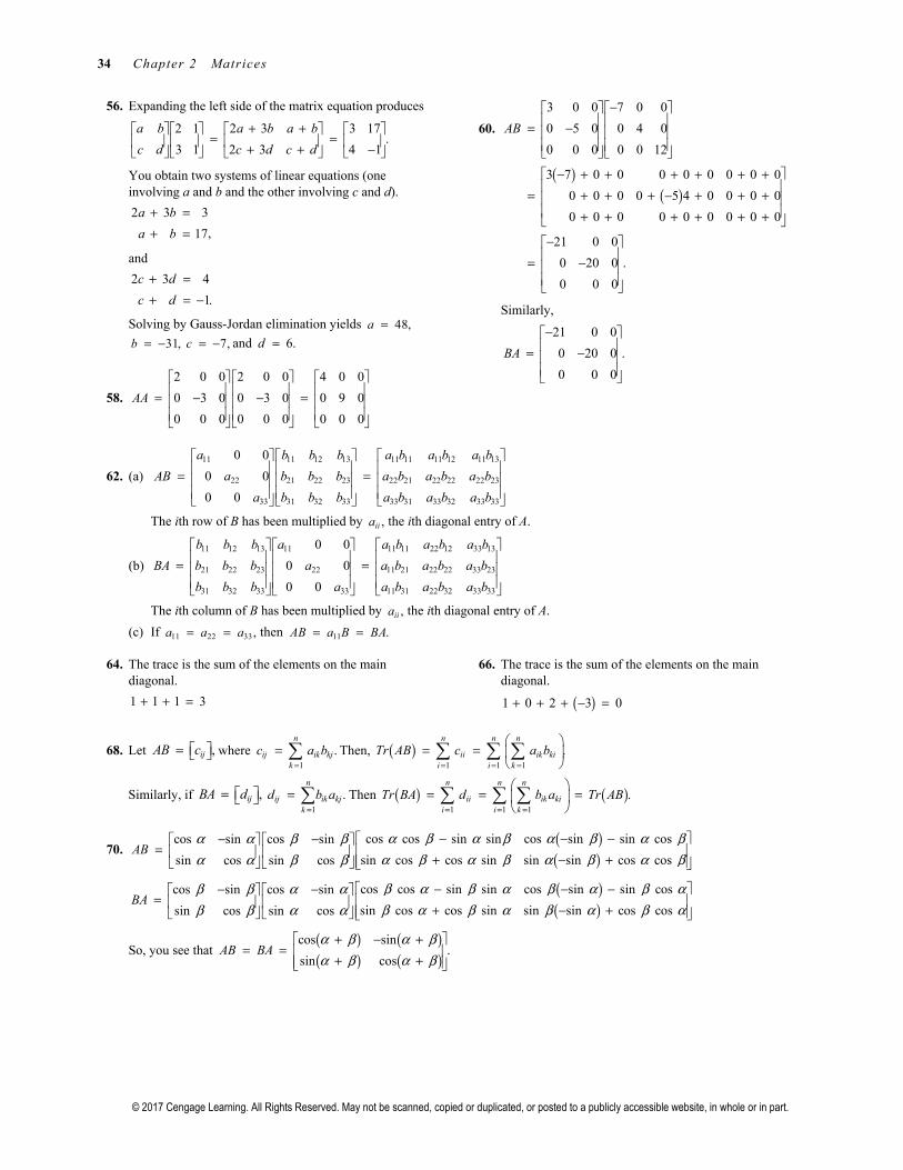
56. Expanding the left side of the matrix equation produces

2 1 2 3 3 17

.3 1 2 3 4 1

a b a b a b

c d c d c d

+ + = = + + −

You obtain two systems of linear equations (one involving a and b and the other involving c and d).

2 3 3

,17

a b

a b

+ =+ =

and

2 3 4

1.

c d

c d

+ =+ = −

Solving by Gauss-Jordan elimination yields 48,a =31,b = − 7,c = − and 6.d =

58.

2 0 0 2 0 0 4 0 0

0 3 0 0 3 0 0 9 0

0 0 0 0 0 0 0 0 0

AA

= − − =

60.

( )( )

3 0 0 7 0 0

0 5 0 0 4 0

0 0 0 0 0 12

3 7 0 0 0 0 0 0 0 0

0 0 0 0 5 4 0 0 0 0

0 0 0 0 0 0 0 0 0

21 0 0

0 20 0 .

0 0 0

AB

− = −

− + + + + + +

= + + + − + + + + + + + + + − = −

Similarly,

21 0 0

0 20 0 .

0 0 0

BA

− = −

62. (a)

11 11 12 13 11 11 11 12 11 13

22 21 22 23 22 21 22 22 22 23

33 31 32 33 33 31 33 32 33 33

0 0

0 0

0 0

a b b b a b a b a b

AB a b b b a b a b a b

a b b b a b a b a b

= =

The ith row of B has been multiplied by ,iia the ith diagonal entry of A.

(b)

11 12 13 11 11 11 22 12 33 13

21 22 23 22 11 21 22 22 33 23

31 32 33 33 11 31 22 32 33 33

0 0

0 0

0 0

b b b a a b a b a b

BA b b b a a b a b a b

b b b a a b a b a b

= =

The ith column of B has been multiplied by ,iia the ith diagonal entry of A.

(c) If 11 22 33,a a a= = then 11 .AB a B BA= =

64. The trace is the sum of the elements on the main diagonal.

1 1 1 3+ + =

66. The trace is the sum of the elements on the main diagonal.

( )1 0 2 3 0+ + + − =

68. Let ,ijAB c = where 1

.n

ij ik kjk

c a b=

= Then, ( )1 1 1

.n n n

ii ik kii i k

Tr AB c a b= = =

= =

Similarly, if ,ijBA d = 1

.n

ij ik kjk

d b a=

= Then ( ) ( )1 1 1

.n n n

ii ik kii i k

Tr BA d b a Tr AB= = =

= = =

70. ( )( )

cos cos sin sin cos sin sin coscos sin cos sin

sin cos cos sin sin sin cos cossin cos sin cosAB

α β α β α β α βα α β βα β α β α β α βα α β β

− − −− − = + − +

( )( )

cos cos sin sin cos sin sin coscos sin cos sin

sin cos cos sin sin sin cos cossin cos sin cosBA

β α β α β α β αβ β α αβ α β α β α β αβ β α α

− − −− − = + − +

So, you see that ( ) ( )( ) ( )

cos sin.

sin cosAB BA

α β α βα β α β

+ − += =

+ +



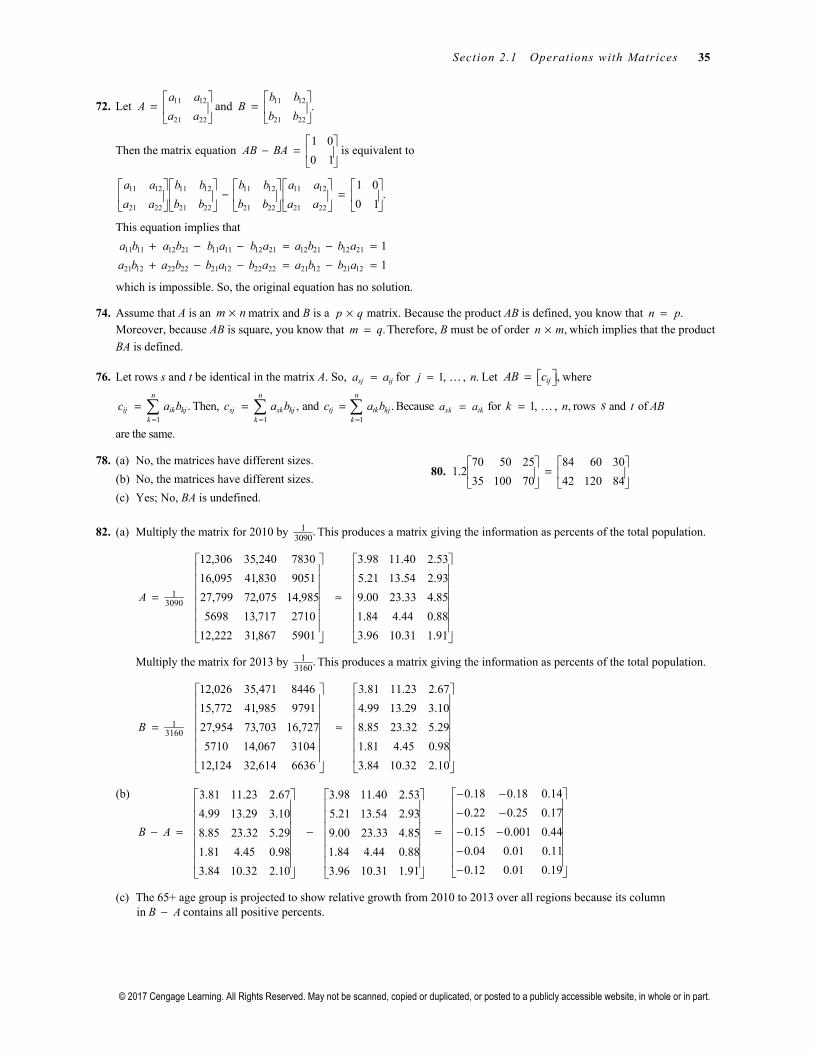
72. Let 11 12

21 22

a aA

a a

=

and 11 12

21 22

.b b

Bb b

=

Then the matrix equation 1 0

0 1AB BA

− =

is equivalent to

11 12 11 12 11 12 11 12

21 22 21 22 21 22 21 22

1 0.

0 1

a a b b b b a a

a a b b b b a a

− =

This equation implies that

11 11 12 21 11 11 12 21 12 21 12 21

21 12 22 22 21 12 22 22 21 12 21 12

1

1

a b a b b a b a a b b a

a b a b b a b a a b b a

+ − − = − =+ − − = − =

which is impossible. So, the original equation has no solution.

74. Assume that A is an m n× matrix and B is a p q× matrix. Because the product AB is defined, you know that .n p= Moreover, because AB is square, you know that .m q= Therefore, B must be of order ,n m× which implies that the product

BA is defined.

76. Let rows s and t be identical in the matrix A. So, sj ija a= for 1, , .j n= Let ,ijAB c = where

1

.n

ij ik kjk

c a b=

= Then, 1

,n

sj sk kjk

c a b=

= and 1

.n

tj tk kjk

c a b=

= Because sk tka a= for 1, , ,k n= rows s and t of AB

are the same.

78. (a) No, the matrices have different sizes.

(b) No, the matrices have different sizes.

(c) Yes; No, BA is undefined.

80. 70 50 25 84 60 30

1.235 100 70 42 120 84

=

82. (a) Multiply the matrix for 2010 by 13090

. This produces a matrix giving the information as percents of the total population.

13090

12,306 35,240 7830 3.98 11.40 2.53

16,095 41,830 9051 5.21 13.54 2.93

27,799 72,075 14,985 9.00 23.33 4.85

5698 13,717 2710 1.84 4.44 0.88

12,222 31,867 5901 3.96 10.31 1.91

A

= ≈

Multiply the matrix for 2013 by 13160

. This produces a matrix giving the information as percents of the total population.

13160

12,026 35,471 8446 3.81 11.23 2.67

15,772 41,985 9791 4.99 13.29 3.10

27,954 73,703 16,727 8.85 23.32 5.29

5710 14,067 3104 1.81 4.45 0.98

12,124 32,614 6636 3.84 10.32 2.10

B

= ≈

(b)

0.18 0.18 0.143.81 11.23 2.67 3.98 11.40 2.53

0.22 0.25 0.174.99 13.29 3.10 5.21 13.54 2.93

8.85 23.32 5.29 9.00 23.33 4.85

1.81 4.45 0.98 1.84 4.44 0.88

3.84 10.32 2.10 3.96 10.31 1.91

B A

− − − − − = − =

0.15 0.001 0.44

0.04 0.01 0.11

0.12 0.01 0.19

− − − −

(c) The 65+ age group is projected to show relative growth from 2010 to 2013 over all regions because its column in B A− contains all positive percents.



84.

0 0 1 0 1 2 3 4 1 2 3 4

0 0 0 1 5 6 7 8 5 6 7 8

1 0 0 0 1 2 3 4 1 2 3 4

0 1 0 0 5 6 7 8 5 6 7 8

AB

= = − − − − − − − − − −

86. (a) True. The number of elements in a row of the first matrix must be equal to the number of elements in a column of the second matrix. See page 43 of the text.

(b) True. See page 45 of the text.

Section 2.2 Properties of Matrix Operations

2. ( ) ( )

( ) ( ) ( )6 0 11 8 5 76 8 0 5 11 7 5 6

1 3 2 0 1 11 0 3 1 2 1 2 2

+ + − + + −− − − + + = = − + − + + − + −− − − − − −

4. [ ] [ ]( ) ( ) [ ] 19 91 1 12 2 2 2 2

5 2 4 0 14 6 18 9 5 14 2 6 4 18 0 9 19 4 14 9 2 7 − + − = + − + + − + = − = −

6. ( ) ( )( )

1 16 6

13

16

4 11 5 1 7 5 4 11 5 7 1 5

1 2 1 3 4 9 1 2 1 3 9 4 1

9 3 0 13 6 1 9 3 0 6 13 1

4 11 2 4 4 11

2 1 6 3 2 1

9 3 6 12 9 3

− − − − − + − + − − − + + − − = + + − + − − − − + + −

− − − − = + − = + − − − −

( )

2312

311 2 113 3 3 3

312 2

1

1 2

4 11

2 1 1 1

9 1 3 2 8 1

−

− + − + − −

= + − + = − + − + − −

8. 1 2 0 1 1 3

3 4 1 2 2 6A B

+ = + = −

10. ( ) ( )( ) ( )0 1 0 1 0 13 4 1

1 2 1 2 1 2a b B

− + = + − = − = − − −

12. ( ) ( )( ) ( )0 0 0 0 0 03 4 12

0 0 0 0 0 0ab O

= − = − =

14. (a) 3 2

6 3 0 6

3 0 4 0

9 12 8 2

6 9

1 0

17 10

X A B= −

− − = − − − −

− = − −

(b)

52

72

2 2

4 2 0 3

2 2 0 2 0

6 8 4 1

4 5

2 0 0

10 7

2

0 0

5

X A B

X

X

X

= −

− − = − − − − − − = −

− −

= −

Section 2.2 Properties of Matrix Operations 37


(c)

12

13 112 2

2 3

6 3 0 3

2 3 0 2 0

9 12 4 1

6 6

2 1 0

13 11

3 3

0

X A B

X

X

X

+ =

− − + = − − −

= − −

= − −

(d) 2 4 2

4 2 0 12

2 0 8 0 2

6 8 16 4

4 10

10 0 2

10 12

2 5

5 0

5 6

A B X

X

X

X

+ = −

− − + = − − − −

− = − − −

− − =

16. ( ) ( )

( )

0 1 1 32

1 0 1 2

1 22

1 3

2 4

2 6

c C B

= − − − −

= − − − = −

18. ( ) 0 1 1 3 0 1

1 0 1 2 1 0

0 1 3 1 2 1

1 0 2 1 3 1

C BC

= − − − − − −

= = − − − −

20. ( ) 1 3 0 1 0 0

1 2 1 0 0 0

1 3 0 1 3 1

1 2 1 0 2 1

B C O

+ = + − − −

= = − − − −

22. ( ) ( )1 3 1 2 32

1 2 0 1 1

1 3 2 4 6 2 10 0

1 2 0 2 2 2 0 10

B cA

= − − − − − − − −

= = − −

24. (a) ( )3 4

4 2 1 5 00 1

1 3 2 3 31 1

3 48 26 6

0 17 14 9

1 1

18 0

12 5

AB C

− − − = − − −

− − = − − −

= −

(b) ( )3 4

4 2 1 5 00 1

1 3 2 3 31 1

4 2 3 1

1 3 3 2

18 0

12 5

A BC

− − − = − − − − − −

= − −

= −

26. 31 1 1 1 1

4 2 2 2 8 431 1 1 1 1

2 2 2 4 2 8

31 1 1 1 12 2 4 2 8 2

31 1 1 1 12 4 2 2 4 8

AB

BA AB

= =

= = ≠

28.

1 2 3 0 0 0 12 6 9

0 5 4 0 0 0 16 8 12

3 2 1 4 2 3 4 2 3

4 6 3 0 0 0

5 4 4 0 0 0

1 0 1 4 2 3

AC

BC

− = = − − − −

− = = − −

But .A B≠

30. 12

1 22 4 0 0

12 4 0 0AB O

− = = = −

But A O≠ and .B O≠



32. 1 2 1 0 1 2

0 1 0 1 0 1AT

= = − −

34. 1 2 1 0 1 2

0 1 0 1 0 1

1 2 1 2 2 4

0 1 0 1 0 2

A IA

+ = + − −

= + = − − −

36. 22

1 2 1 2 1 0

0 1 0 1 0 1A I

= = = − −

So, ( )24 2 22 2

1 0.

0 1A A I I

= = = =

38. In general, AB BA≠ for matrices.

40.

6 7 19 6 7 19

7 0 23 7 0 23

19 23 32 19 23 32

T

TD

− − = − = − − −

42. ( ) 1 2 3 1 1 1 1 4

0 2 2 1 4 2 1 2

3 1 1 2 3 2 1 0 1 4

2 1 0 2 1 1 2 2 1 2

T TT

T T

T T

AB

B A

− − − = = = − − − −

− − − − = = = − − − −

44. ( )2 1 1 1 0 1 4 0 7 4 2 4

0 1 3 2 1 2 2 4 7 0 4 2

4 0 2 0 1 3 4 2 2 7 7 2

1 0 1 2 1 1 1 2 0 2 0 4 4 2 4

2 1 2 0 1 3 0 1 1 1 1 0 0 4 2

0 1 3 4 0 2 1 2 3 1 3 2 7 7 2

T T

T

T T

T T

AB

B A

− − − = − = = −

− − = − = = − − − −

46. (a)

1 11 3 0 10 11

3 41 4 2 11 21

0 2

TA A

− = = − − −

(b)

1 1 2 1 21 3 0

3 4 1 25 81 4 2

0 2 2 8 4

TAA

− − = = − − − − − −

48. (a)

4 2 14 6 4 3 2 0 252 8 168 104

3 0 2 8 2 0 11 1 8 77 70 50

2 11 12 5 14 2 12 9 168 70 294 139

0 1 9 4 6 8 5 4 104 50 139 98

TA A

− − − − − − = = − − − − − − − − − −

(b)

4 3 2 0 4 2 14 6 29 30 86 10

2 0 11 1 3 0 2 8 30 126 169 47

14 2 12 9 2 11 12 5 86 169 425 28

6 8 5 4 0 1 9 4 10 47 28 141

TAA

− − − − − − = = − − − − − − − − − −

50. ( )( )

( )( )

( )

17

17

1717

17

17

0 0 0 01 1 0 0 0 0

0 1 0 0 00 0 0 010 0 1 0 00 0 0 010 0 0 1 0

0 0 0 01 0 0 0 0 10 0 0 0 1

A

− − == − −

Section 2.2 Properties of Matrix Operations 39


52. ( )( )

( )( )

( )

20

20

2020

20

20

0 0 0 01 1 0 0 0 0

0 1 0 0 00 0 0 010 0 1 0 00 0 0 010 0 0 1 0

0 0 0 01 0 0 0 0 10 0 0 0 1

A

− == −

54. Because ( )( )

3

33

3

2 0 08 0 0

0 1 0 0 1 0 ,

0 0 27 0 0 3

A

= − = −

you have

2 0 0

0 1 0 .

0 0 3

A

= −

56. (a) False. In general, for n n× matrices A and B it is not true that .AB BA= For example, let 1 1 1 0

, .0 0 1 0

A B

= =

Then 2 0 1 1

.0 0 1 1

AB BA

= ≠ =

(b) False. Let 1 1 1 0 2 0

, , .0 0 1 0 0 0

A B C

= = =

Then 2 0

,0 0

AB AC

= =

but .B C≠

(c) True. See Theorem 2.6, part 2 on page 57.

58. ( ) ( )( ) ( )

( ) ( )

Original equation

Associative property; property of the identity matrix

Property of scalar multiplication; distributive property

Add to b

aX A bB b AB IB

aX Ab B b AB B

aX bAB bAB bB

aX bAB bAB bAB bB bAB bAB

+ = ++ = +

+ = ++ + − = + + − −

( )( )

oth sides.

Additive inverse

Commutative property

Additive inverse

Divide by .

aX bAB bB bAB

aX bAB bAB bB

aX bB

bX B a

a

= + + −= + − +=

=

60. ( )

2 31 0 0 2 1 1 2 1 1 2 1 1

10 0 1 0 5 1 0 2 2 1 0 2 1 0 2

0 0 1 1 1 3 1 1 3 1 1 3

10 0 0 10 5 5 2 1 1 2 1 1 2 1 1

0 10 0 5 0 10 2 1 0 2 1 0 2 1 0 2

0 0 10 5 5 15 1 1 3 1 1 3 1 1 3

f A

− − − = − + − + − − −

− − − − = − + − + − − − −

22 1 1

1 0 2

1 1 3

0 5 5 6 1 3 2 1 1 6 1 3

5 10 10 2 0 3 5 1 0 2 0 3 5

5 5 5 4 2 12 1 1 3 4 2 12

0 5 5 12 2 6 16 3 13

5 10 10 0 6 10 2 5 21

5 5 5 8 4 24 18 8 44

− −

− − − − = − − + − − − −

− − − = − − + − − − −

4 6 12

3 11 21

15 9 25

− = − −



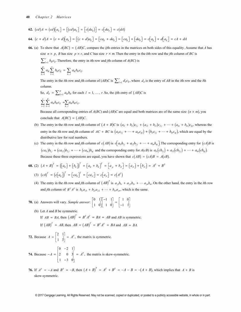
62. ( ) ( ) ( ) ( ) ( )ij ij ij ijcd A cd a cd a c da c da c dA = = = = =

64. ( ) ( ) ( )ij ij ij ij ij ij ij ijc d A c d a c d a ca da ca da c a d a cA dA + = + = + = + = + = + = +

66. (a) To show that ( ) ( ) ,A BC AB C= compare the ijth entries in the matrices on both sides of this equality. Assume that A has

size ,n p B× has size ,p r× and C has size .r m× Then the entry in the kth row and the jth column of BC is

1

.r

kl ljlb c

= Therefore, the entry in ith row and jth column of A(BC) is

1 1 ,

.p r

ik kl lj ik kl ljk l k l

a b c a b c= =

=

The entry in the ith row and jth column of (AB)C is 1

,r

il ljld c

= where ild is the entry of AB in the ith row and the lth

column.

So, 1

pil ik klk

d a b=

= for each 1, , .l r= So, the ijth entry of ( )AB C is

1 1 ,

.pr

ik kl lj ik kl iji k k l

a b c a b c= =

=

Because all corresponding entries of A(BC) and (AB)C are equal and both matrices are of the same size ( ),n m× you

conclude that ( ) ( ) .A BC AB C=

(b) The entry in the ith row and jth column of ( )A B C+ is ( ) ( ) ( )1 2 2 2 ,il il j i i j in in nja b c a b c a b c+ + + + + + whereas the

entry in the ith row and jth column of AC BC+ is ( ) ( )1 1 1 1 ,i j in nj i j in nja c a c b c b c+ + + + + which are equal by the

distributive law for real numbers.

(c) The entry in the ith row and jth column of ( )c AB is 1 1 2 2 .i j i j in njc a b a b a b + + + The corresponding entry for ( )cA B is

( ) ( ) ( )1 1 2 2i j i j in njca b ca b ca b+ + + and the corresponding entry for A(cB) is ( ) ( ) ( )1 1 2 2 .i j i j in nja cb a cb a cb+ + +

Because these three expressions are equal, you have shown that ( ) ( ) ( ).c AB cA B A cB= =

68. (2) ( ) ( )T TT T Tij ij ij ij ji ji jijiA B a b a b a b a b A B + = + = + = + = + = +

(3) ( ) ( ) ( )T TT Tij ij ji jicA c a ca ca c a c A = = = = =

(4) The entry in the ith row and jth column of ( )TAB is 1 1 2 2 .j i j i jn nia b a b a b+ + On the other hand, the entry in the ith row

and jth column of T TB A is 1 1 2 2 ,i j i j ni jnb a b a b a+ + + which is the same.

70. (a) Answers will vary. Sample answer: 0 1 1 1 1 0

1 0 1 0 1 1

− = −

(b) Let A and B be symmetric.

If ,AB BA= then ( )T T TAB B A BA AB= = = and AB is symmetric.

If ( ) ,T

AB AB= then ( )T T TAB AB B A BA= = = and .AB BA=

72. Because 2 1

,1 3

TA A

= =

the matrix is symmetric.

74. Because

0 2 1

2 0 3 ,

1 3 0

TA A

− − = = −

the matrix is skew-symmetric.

76. If TA A= − and ,TB B= − then ( ) ( ),T T TA B A B A B A B+ = + = − − = − + which implies that A B+ is

skew-symmetric.

Section 2.3 The Inverse of a Matrix 41


78. Let 11 12 13 1

21 22 23 2

1 2 3

11 12 13 1 11 21 31 1

21 22 23 2 12 22 32 2

1 2 3 1 2 3

12 21 13 31 1

.

0

n

n

n n n nn

Tn n

n n

n n n nn n n n nn

n

A a a a a

a a a a

a a a a

A A a a a a a a a a

a a a a a a a a

a a a a a a a a

a a a a a

=

− = −

− −

=

( )

( ) ( ) ( )

1

21 12 23 32 2 2

1 1 2 2 3 3

12 21 13 31 1 1

23 32 2 212 21

1 1 2 2 3 3

0

0

0

0

0

n

n n

n n n n n n

n n

n n

n n n n n n

a

a a a a a a

a a a a a a

a a a a a a

a a a aa a

a a a a a a

− − − − − − −

− − − − −− − = − − − − − −

So, TA A− is skew-symmetric.

Section 2.3 The Inverse of a Matrix

2. 1 1 2 1 2 1 1 1 1 0

1 2 1 1 2 2 1 2 0 1

2 1 1 1 2 1 2 2 1 0

1 1 1 2 1 1 1 2 0 1

AB

BA

− − − = = = − − + − +

− − − + = = = − − − +

4. 3 15 52 15 5

3 15 52 15 5

1 1 1 0

2 3 0 1

1 1 1 0

2 3 0 1

AB

BA

− = = −

− = = −

6.

2 17 11 1 1 2 1 0 0

1 11 7 2 4 3 0 1 0

0 3 2 3 6 5 0 0 1

1 1 2 2 17 11 1 0 0

2 4 3 1 11 7 0 1 0

3 6 5 3 6 2 0 0 1

AB

BA

− = − − − = − −

− = − − − = − −

8. Use the formula

1 1,

d bA

ad bc c a− −

= − −

where

2 2

.2 2

a bA

c d

− = =

So, the inverse is

( ) ( )( )

1

1 12 21 4 4 .

2 2 2 2 2 2 1 1

4 4

A−

= = − − − −

10. Use the formula

1 1,

d bA

ad bc c a− −

= − −

where

1 2

.2 3

a bA

c d

− = = −

So, the inverse is

( )( ) ( )( )1

3 2 3 21.

1 3 2 2 2 1 2 1A− − −

= = − − − − −



12. Using the formula

1 1,

d bA

ad bc c a− −

= − −

where

1 1

3 3

a bA

c d

− = = −

you see that ( )( ) ( )( )1 3 1 3 0.ad bc− = − − − = So, the

matrix has no inverse.

14. Adjoin the identity matrix to form

[ ]1 2 2 1 0 0

3 7 9 0 1 0 .

1 4 7 0 0 1

A I

= − − −

Using elementary row operations, reduce the matrix as follows.

1

1 0 0 13 6 4

0 1 0 12 5 3

0 0 1 5 2 1

I A−

− = − − −


[ ]10 5 7 1 0 0

5 1 4 0 1 0 .

3 2 2 0 0 1

A I

− = − −


1

1 0 0 10 4 27

0 1 0 2 1 5

0 0 1 13 5 35

I A−

− − = − − −

Therefore, the inverse is

1

10 4 27

2 1 5 .

13 5 35

A−

− − = − − −


[ ]3 2 5 1 0 0

2 2 4 0 1 0 .

4 4 0 0 0 1

A I

= −

Using elementary row operations, you cannot form the identity matrix on the left side. Therefore, the matrix has no inverse.


[ ]5 1 116 3 6

23

512 2

1 0 0

0 2 0 1 0 .

1 0 0 1

A I

−

= − −



[ ]0.1 0.2 0.3 1 0 0

0.3 0.2 0.2 0 1 0 .

0.5 0.5 0.5 0 0 1

A I

= −


1

1 0 0 0 2 0.8

0 1 0 10 4 4.4

0 0 1 10 2 3.2

I A−

− = − − −


1

0 2 0.8

10 4 4.4 .

10 2 3.2

A−

− = − − −


[ ]1 0 0 1 0 0

3 0 0 0 1 0

2 5 5 0 0 1

A I

=



[ ]

1 0 0 0 1 0 0 0

0 2 0 0 0 1 0 0.

0 0 2 0 0 0 1 0

0 0 0 3 0 0 0 1

A I

= −


112

12

13

1 0 0 0 1 0 0 0

0 1 0 0 0 0 0

0 0 1 0 0 0 0

0 0 0 1 0 0 0

I A−

= −


112

12

13

1 0 0 0

0 0 0.

0 0 0

0 0 0

A−

= −




[ ]

4 8 7 14 1 0 0 0

2 5 4 6 0 1 0 0.

0 2 1 7 0 0 1 0

3 6 5 10 0 0 0 1

A I

− − = − −


[ ]

1 0 0 0 27 10 4 29

0 1 0 0 16 5 2 18

0 0 1 0 17 4 2 20

0 0 0 1 7 2 1 8

A I

− − − − = − − − −

Therefore the inverse is

1

27 10 4 29

16 5 2 18.

17 4 2 20

7 2 1 8

A−

− − − − = − − − −


[ ]

1 3 2 0 1 0 0 0

0 2 4 6 0 1 0 0.

0 0 2 1 0 0 1 0

0 0 0 5 0 0 0 1

A I

− = −


1

1 0 0 0 1 1.5 4 2.6

0 1 0 0 0 0.5 1 0.8.

0 0 1 0 0 0 0.5 0.1

0 0 0 1 0 0 0 0.2

I A−

− − − = −


1

1 1.5 4 2.6

0 0.5 1 0.8.

0 0 0.5 0.1

0 0 0 0.2

A−

− − − = −

32. 1 2

3 2A

− = −

( )( ) ( )( )1 2 2 3 4ad bc− = − − − = −

11 1

1 2 23 144 4

2 2

3 1A−

− − = − = − −

34. 12 3

5 2A

− = −

( )( ) ( )12 2 3 5 24 15 9ad bc− = − − − = − =

12 19 31

9 5 49 3

2 3

5 12A−

− −− − = = − − − −

36. 91

4 45 83 9

A −

=

( )( ) ( )( )8 9 5 14314 9 4 3 36

ad bc− = − − = −

18 9 32 819 4 143 14336

143 5 60 913 4 143 143

A− − − = − = − −

38. ( )

( )

222 1

112 2

1 147 2209

12209

6 7 1 56

5 2 40 31

31 56 1 56

40 1 40 31

A A

A A

− −

−−−

− − = = = −

− − = = = − −

The results are equal.

40. ( )

( )

2

22 1

1

12 2

1 12 4

14

15 4 28 873 228 1604

1 0 2 61 16 112

23 6 42 1317 344 2420

48 4 32 873 228 1604

29 48 17 61 16 112

22 9 15 1317 344 2420

A A

A A

− −

−

−−

− − − = = − = − − − −

− = = − − = − − −

The results are equal.



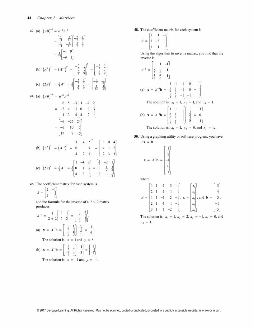
42. (a) ( ) 1 1 1

5 2 127 711 1133 217 711 11

177

4 9

9 1

AB B A− − −=

−=

− −

= −

(b) ( ) ( )1 132 1 2

7 7 7 73 2 1 27 7 7 7

TTTA A

− − − −

= = =

(c) ( ) 1 12 1 1 17 7 7 141 1

2 2 3 32 17 7 14 7

2A A− −

− −= = =

44. (a) ( ) 1 1 1

6 5 3 1 4 2

2 4 1 0 1 3

1 3 4 4 2 1

6 25 24

6 10 7

17 7 15

AB B A− − −=

− − = − − − − = −

(b) ( ) ( )1 1

1 4 2 1 0 4

0 1 3 4 1 2

4 2 1 2 3 1

T

TTA A− −

− = = = −

(c) ( ) 1 1

12

31 1 12 2 2 2

12

1 4 2 2 1

2 0 1 3 0

4 2 1 2 1

A A− −

− − = = =

46. The coefficient matrix for each system is

2 1

2 1A

− =

and the formula for the inverse of a 2 2× matrix produces

11 14 41 12 2

1 11.

2 2 2 2A−

= = + −−

(a) 11 14 41 12 2

3 1

7 5A−

− = = = −

x b

The solution is: 1x = and 5.y =

(b) 11 14 41 12 2

1 1

3 1A−

− − = = = − − −

x b

The solution is: 1x = − and 1.y = −

48. The coefficient matrix for each system is

1 1 2

1 2 1 .

1 1 1

A

− = − − −

Using the algorithm to invert a matrix, you find that the inverse is

1 2 13 31 23 3

1 1 1

1 .

1

A−

−

= − −

(a) 1 2 13 31 23 3

1 1 1 0 1

1 0 1

1 1 1

A−

− = = − = − −

x b

The solution is: 1 1,x = 2 1,x = and 3 1.x =

(b) 1 2 13 31 23 3

1 1 1 1 1

1 2 0

1 0 1

A−

− − = = − = −

x b

The solution is: 1 1,x = 2 0,x = and 3 1.x =

50. Using a graphing utility or software program, you have

1

1

2

1

0

1

A

A

x b

x b−

=

= = −

where

1 1 1 3 1

2 1 1 1 1

,1 1 1 2 1

2 1 4 1 1

3 1 1 2 1

A

− − = − − −

−

1

2

3

4

5

,

x

x

x

x

x

=

x and

3

4

.3

1

5

= −

b

The solution is: 1 2 3 41, 2, 1, 0,x x x x= = = − = and

5 1.x =



52. Using a graphing utility or software program, you have

1

1

2

1

3

0

1

A

A

x b

x b−

=

− = =

where

1

2

3

4

5

6

4 2 4 2 5 1

3 6 5 6 3 3

2 3 1 3 1 2, ,

1 4 4 6 2 4

3 1 5 2 3 5

2 3 4 6 1 2

x

x

xA

x

x

x

− − − − − − − − = =− − − − − − − − −

x and

1

11

0.

9

1

12

− = − −

b

The solution is: 1 1,x = − 2 2,x = 3 1,x = 4 3,x =

5 0,x = and 6 1.x =

54. The inverse of A is given by

121

.4 1 2

xA

x− − −

= −

Letting 1 ,A A− = you find that 1

1.4x

= −−

So, 3.x =

56. The matrix 2

3 4

x −

will be singular if

( )( ) ( )( )4 3 2 0,ad bc x− = − − = which implies that

4 6x = − or 32.x = −

58. First, find 4 .A

( )11

1 18 43 1

16 8

2 414 4

4 12 3 2A A

−− −− = = = +

Then, multiply by 14 to obtain

( )1 1 1 18 4 32 161 1

4 4 3 31 116 8 64 32

4 .A A − −

= = =

60. Using the formula for the inverse of a 2 2× matrix, you have

1

2 2

1

sec tan1

sec tan tan sec

sec tan.

tan sec

d bA

ad bc c a

θ θθ θ θ θ

θ θθ θ

− − = − −

− = − −

− = −


[ ]0.017 0.010 0.008 1 0 0

0.010 0.012 0.010 0 1 0 .

0.008 0.010 0.017 0 0 1

F I

=


1

1 0 0 115.56 100 4.44

0 1 0 100 250 100

0 0 1 4.44 100 115.56

I F −

− = − − −

So, 1

115.56 100 4.44

100 250 100

4.44 100 115.56

F −

− = − − −

and

1

115.56 100 4.44 0 15

100 250 100 0.15 37.5 .

4.44 100 115.56 0 15

F −

− − = = − − = − −

w d

64. ( ) ( )1 1T TT Tn nA A A A I I− −= = = and

( ) ( )1 1T TT Tn nA A AA I I− −= = =

So, ( ) ( ) 11 .T TA A

−− =

66. ( )( )

( )

2 2

2

2

2 2 2 2 4

4 4

4 4 because

I A I A I IA AI A

I A A

I A A A A

I

− − = − − +

= − +

= − + =

=

So, ( ) 12 2 .I A I A

−− = −

68. Because ,ABC I A= is invertible and 1 .A BC− =

So, ABC A A= and .BC A I=

So, 1 .B CA− =

70. Let 2A A= and suppose A is nonsingular. Then, 1A−

exists, and you have the following.

( )( )

1 2 1

1

A A A A

A A A I

A I

− −

−

=

=

=



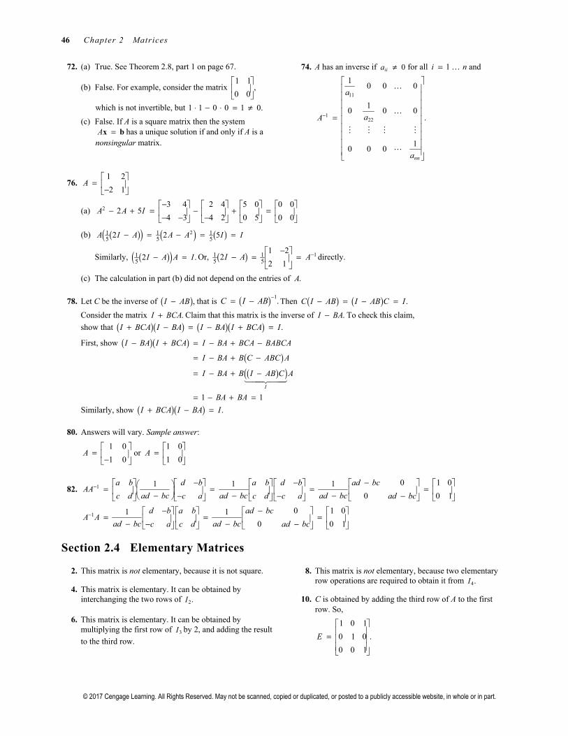
72. (a) True. See Theorem 2.8, part 1 on page 67.

(b) False. For example, consider the matrix 1 1

,0 0

which is not invertible, but 1 1 0 0 1 0.⋅ − ⋅ = ≠

(c) False. If A is a square matrix then the system A =x b has a unique solution if and only if A is a

nonsingular matrix.

74. A has an inverse if 0iia ≠ for all 1i n= and

11

122

10 0 0

10 0 0

.

10 0 0

nn

a

aA

a

−

=

76. 1 2

2 1A

= −

(a) 23 4 2 4 5 0 0 0

2 54 3 4 2 0 5 0 0

A A I−

− + = − + = − − −

(b) ( )( ) ( ) ( )21 1 15 5 5

2 2 5A I A A A I I− = − = =

Similarly, ( )( )15

2 .I A A I− = Or, ( ) 11 15 5

1 22

2 1I A A−−

− = =

directly.

(c) The calculation in part (b) did not depend on the entries of .A

78. Let C be the inverse of ( ),I AB− that is ( ) 1.C I AB

−= − Then ( ) ( ) .C I AB I AB C I− = − =

Consider the matrix .I BCA+ Claim that this matrix is the inverse of .I BA− To check this claim,

show that ( )( ) ( )( ) .I BCA I BA I BA I BCA I+ − = − + =

First, show ( )( )( )( )( )

1 1I

I BA I BCA I BA BCA BABCA

I BA B C ABC A

I BA B I AB C A

BA BA

− + = − + −

= − + −

= − + −

= − + =

Similarly, show ( )( ) .I BCA I BA I+ − =

80. Answers will vary. Sample answer:

1 0

1 0A

= −

or 1 0

1 0A

=

82. 1

1

0 1 01 1 1

0 0 1

0 1 01 1

0 0 1

a b d b a b d b ad bcAA

ad bc ad bc ad bcc d c a c d c a ad bc

d b a b ad bcA A

ad bc ad bcc a c d ad bc

−

−

− − − = = = = − − −− − − − −

= = = − −− −

Section 2.4 Elementary Matrices

2. This matrix is not elementary, because it is not square.

4. This matrix is elementary. It can be obtained by interchanging the two rows of 2.I

6. This matrix is elementary. It can be obtained by multiplying the first row of 3I by 2, and adding the result

to the third row.

8. This matrix is not elementary, because two elementary row operations are required to obtain it from 4.I

10. C is obtained by adding the third row of A to the first row. So,

1 0 1

0 1 0 .

0 0 1

E

=

Section 2.4 Elementary Matrices 47


12. A is obtained by adding 1− times the third row of C to the first row. So,

1 0 1

0 1 0 .

0 0 1

E

− =


Matrix Elementary Row Operation Elementary Matrix

1 1 2 2

0 3 3 6

0 0 2 2

− − −

1 2R R↔ 0 1 0

1 0 0

0 0 1

1 1 2 2

0 1 1 2

0 0 2 2

− − −

( ) 2 213 R R→

13

1 0 0

0 0

0 0 1

1 1 2 2

0 1 1 2

0 0 1 1

− − −

( ) 3 312

R R→

12

1 0 0

0 1 0

0 0

So, 13

12

1 0 0 1 0 0 0 1 0 0 3 3 6 1 1 2 2

0 1 0 0 0 1 0 0 1 1 2 2 0 1 1 2 .

0 0 0 0 1 0 0 1 0 0 2 2 0 0 1 1

− − − − − = −



1 3 0

0 1 1

3 2 4

− − − −

( ) 1 2 22 R R R− + →

1 0 0

2 1 0

0 0 1

−

1 3 0

0 1 1

0 11 4

− − − −

( ) 1 3 33 R R R− + →

1 0 0

0 1 0

3 0 1

−

1 3 0

0 1 1

0 11 4

− −

( ) 2 21 R R− →

1 0 0

0 1 0

0 0 1

−

1 3 0

0 1 1

0 0 7

( ) 2 3 311 R R R+ →

1 0 0

0 1 0

0 11 1

1 3 0

0 1 1

0 0 1

( ) 3 317

R R→

17

1 0 0

0 1 0

0 0

So, 17

1 0 0 1 0 0 1 0 0 1 0 0 1 0 0 1 3 0 1 3 0

0 1 0 0 1 0 0 1 0 0 1 0 2 1 0 2 5 1 0 1 1 .

0 0 0 11 1 0 0 1 3 0 1 0 0 1 3 2 4 0 0 1

− − − = − − −



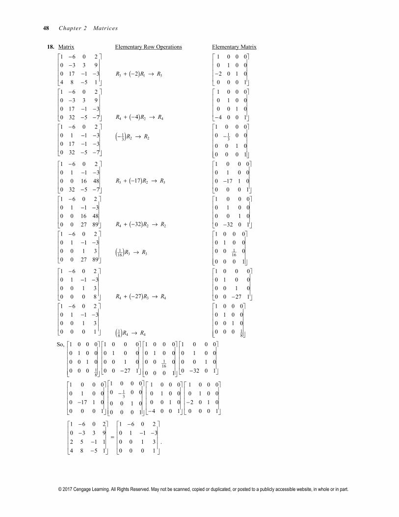
18. Matrix Elementary Row Operations Elementary Matrix

( )

( )

( )

3 1 3

4 2 4

2 211

3

1 6 0 2 1 0 0 0

0 3 3 9 0 1 0 0

20 17 1 3 2 0 1 0

4 8 5 1 0 0 0 1

1 6 0 2 1 0 0 0

0 3 3 9 0 1 0 0

0 17 1 3 0 0 1 040 32 5 7 4 0 0 1

1 6 0 2 1 0 0 0

0 1 1 3 0

0 17 1 3

0 32 5 7

R R R

R R R

R R

− −

+ − →− − − −

− −

− − + − →− − −

− − − −− →

− − − −

( )

( )

3 2 3

4 2 2

30 0

0 0 1 0

0 0 0 1

1 6 0 2 1 0 0 0

0 1 1 3 0 1 0 0170 0 16 48 0 17 1 0

0 32 5 7 0 0 0 1

1 6 0 2 1 0 0 0

0 1 1 3 0 1 0 0

0 0 16 48 0 0 1 0320 0 27 89 0 32 0 1

1 6 0 2

0 1 1 3

0 0 1 3

0 0 27 89

R R R

R R R

− − −

+ − → − − −

− − − + − → −

−− −

( )

( )

( )

3 3

4 3 4

4 4

111616

1188

1 0 0 0

0 1 0 0

0 0 0

0 0 0 1

1 6 0 2 1 0 0 0

0 1 1 3 0 1 0 0

0 0 1 3 0 0 1 0270 0 0 8 0 0 27 1

1 6 0 2 1 0 0 0

0 1 1 3 0 1 0 0

0 0 1 3 0 0 1 0

0 0 0 1 0 0 0

R R

R R R

R R

→

− − − + − → −

− − −

→

So,

116

18

13

1 0 0 0 1 0 0 0 1 0 0 0 1 0 0 0

0 1 0 0 0 1 0 0 0 1 0 0 0 1 0 0

0 0 1 0 0 0 1 0 0 0 0 0 0 1 0

0 0 0 0 0 27 1 0 32 0 10 0 0 1

1 0 0 01 0 0 0 1 0 0 00 0 00 1 0 0 0 1 0 0

0 17 1 0 0 0 1 00 0 1 00 0 0 1 4 00 0 0 1

− −

− −

−

1 0 0 0

0 1 0 0

2 0 1 0

0 1 0 0 0 1

−

1 6 0 2 1 6 0 2

0 3 3 9 0 1 1 3

2 5 1 1 0 0 1 3 .

4 8 5 1 0 0 0 1

− − − − − = − −



20. To obtain the inverse matrix, reverse the elementary row operation that produced it. So, multiply the

first row by 125 to obtain

115 0

.0 1

E− =

22. To obtain the inverse matrix, reverse the elementary row operation that produced it. So, add 3 times the second row to the third row to obtain

1

1 0 0

0 1 0 .

0 3 1

E−

=

24. To obtain the inverse matrix, reverse the elementary row operation that produced it. So, add k− times the third row to the second row to obtain

1

1 0 0 0

0 1 0.

0 0 1 0

0 0 0 1

kE−

− =

26. Find a sequence of elementary row operations that can be used to rewrite A in reduced row-echelon form.

( ) 1 1

2 1 2

121 0

1 1

1 0

0 1

R R

R R R

→

− →

1

2

12

0

0 1

1 0

1 1

E

E

=

= −

Use the elementary matrices to find the inverse.

12 1

112212

01 0 0

11 1 0 1A E E−

= = = −−


( )

( )

2 2

1 3 1

2 3 2

1 12 2

12

1 12 2

1 0 2

0 1

0 0 1

1 0 0 2

0 1

0 0 1

1 0 0

0 1

0 0 1

R R

R R R

R R R

− →

+ →

− →

1

2

3

12

12

1 0 0

0 0

0 0 1

1 0 2

0 1 0

0 0 1

1 0 0

0 1

0 0 1

E

E

E

=

=

= −

Use the elementary matrices to find the inverse.

13 2 1

1 12 2

1 1 1 12 2 2 2

1 0 0 1 0 2 1 0 0

0 1 0 1 0 0 0

0 0 1 0 0 1 0 0 1

1 0 2 1 0 0 1 0 2

0 1 0 0 0

0 0 1 0 0 1 0 0 1

A E E E−

= = −

= − = −



For Exercises 30–36, answers will vary. Sample answers are shown below.

30. The matrix 0 1

1 0A

=

is itself an elementary matrix, so the factorization is

0 1

.1 0

A

=

32. Reduce the matrix 1 1

2 1A

=

as follows.


1 1

0 1

−

Add 2− times row one to row two. 1

1 0

2 1E

= −

1 1

0 1

Multiply row two by 1.− 2

1 0

0 1E

= −

1 0

0 1

Add 1− times row two to row one. 3

1 1

0 1E

− =

So, one way to factor A is

1 1 11 2 3

1 0 1 0 1 1.

2 1 0 1 0 1A E E E− − −

= = −

34. Reduce the matrix

1 2 3

2 5 6

1 3 4

A

=

as follows.


1 2 3

0 1 0

1 3 4

Add 2− times row one to row two. 1

1 0 0

2 1 0

0 0 1

E

= −

1 2 3

0 1 0

0 1 1

Add 1− times row one to row three. 2

1 0 0

0 1 0

1 0 1

E

= −

1 2 3

0 1 0

0 0 1

Add 1− times row two to row three. 3

1 0 0

0 1 0

0 1 1

E

= −

1 2 0

0 1 0

0 0 1

Add 3− times row three to row one. 4

1 0 3

0 1 0

0 0 1

E

− =

1 0 0

0 1 0

0 0 1

Add 2− times row two to row one. 5

1 2 0

0 1 0

0 0 1

E

− =


1 1 1 1 11 2 3 4 5A E E E E E− − − − −=

1 0 0 1 0 0 1 0 0 1 0 3 1 2 0

2 1 0 0 1 0 0 1 0 0 1 0 0 1 0 .

0 0 1 1 0 1 0 1 1 0 0 1 0 0 1

=




( )

( )

( )

1 1

4 1 4

4 4

3 3

1 4

1142

12

52

12

25

12

12

1 0 0

0 1 0 1

0 0 1 2

1 0 0 2

1 0 0

0 1 0 1

0 0 1 2

0 0 0

1 0 0

0 1 0 1

0 0 1 2

0 0 0 1

1 0 0

0 1 0 1

0 0 1 2

0 0 0 1

1 0 0 0

0 1 0 1

0 0 1 2

0 0 0 1

R R

R R R

R R

R R

R R R

→ − −

− − − →

− − →

− →−

− → −

1

2 4 2

3 4 3

1 0 0 0

0 1 0 0

0 0 1 2

0 0 0 1

1 0 0 0

0 1 0 0

0 0 1 0 2

0 0 0 1

R R R

R R R

− → −

+ →

1

2

3

4

5

6

14

25

12

0 0 0

0 1 0 0

0 0 1 0

0 0 0 1

1 0 0 0

0 1 0 0

0 0 1 0

1 0 0 1

1 0 0 0

0 1 0 0

0 0 1 0

0 0 0

1 0 0 0

0 1 0 0

0 0 1 0

0 0 0 1

1 0 0

0 1 0 0

0 0 1 0

0 0 0 1

1 0 0 0

0 1 0 1

0 0 1 0

0 0 0 1

E

E

E

E

E

E

=

= −

= −

= −

− =

−=

7

1 0 0 0

0 1 0 0

0 0 1 2

0 0 0 1

E

=


1 1 1 1 1 1 11 2 3 4 5 6 7

12

52

1 0 0 04 0 0 0 1 0 0 0 1 0 0 0 1 0 0 01 0 0

0 1 0 00 1 0 0 0 1 0 0 0 1 0 0 0 1 0 10 1 0 0

0 0 1 00 0 1 0 0 0 1 0 0 0 1 0 0 0 1 00 0 1 0

0 0 00 0 0 1 1 0 0 1 0 0 0 1 0 0 00 0 0 1

A E E E E E E E− − − − − − −=

= − −

1 0 0 0

0 1 0 0.

0 0 1 2

1 0 0 0 1

−

38. (a) EA has the same rows as A except the two rows that are interchanged in E will be interchanged in EA.

(b) Multiplying a matrix on the left by E interchanges the same two rows that are interchanged from nI in E.

So, multiplying E by itself interchanges the rows twice and 2 .nE I=



40.

1 1 1

1

1 0 0 1 01 0 0 1 0 0 1 0 1 0 0 1 0

0 1 0 1 0 0 1 0 0 1 0 1 0 0 1 0 1 0 .

0 0 0 0 1 0 0 1 0 0 1 0 0 11 1

0 0 0 0

aa a

A b b b ab

c

c c

− − −

−

− −

= = − = − +

42. (a) False. It is impossible to obtain the zero matrix by applying any elementary row operation to the identity matrix.

(b) True. If 1 2 ,kA E E E= where each iE is an

elementary matrix, then A is invertible (because every elementary matrix is) and

1 1 1 12 1 .kA E E E− − − −=

(c) True. See equivalent conditions (2) and (3) of Theorem 2.15.

44. Matrix Elementary Matrix

2 1

6 4

2 1

0 1

A

U

− = −

− =

1

1 0

3 1E

= −

11 1

1 0 2 1

3 1 0 1E A U A E U LU− −

= = = =


2 0 0

0 3 1

10 12 3

2 0 0

0 3 1

0 12 3

2 0 0

0 3 1

0 0 7

A

U

− =

−

− =

1

2

1 0 0

0 1 0

5 0 1

1 0 0

0 1 0

0 4 1

E

E

= −

=

1 12 1 1 2

1 0 0 2 0 0

0 1 0 0 3 1

5 4 1 0 0 7

E E A U A E E U

LU

− −= =

= − −

=


2 0 0 0

2 1 1 0

6 2 1 0

0 0 0 1

2 0 0 0

0 1 1 0

6 2 1 0

0 0 0 1

2 0 0 0

0 1 1 0

0 2 1 0

0 0 0 1

2 0 0 0

0 1 1 0

0 0 3 0

0 0 0 1

A

U

− − = −

− −

− −

− = −

1

2

3

1 0 0 0

1 1 0 0

0 0 1 0

0 0 0 1

1 0 0 0

0 1 0 0

3 0 1 0

0 0 0 1

1 0 0 0

0 1 0 0

0 2 1 0

0 0 0 1

E

E

E

=

= −

= −

1 1 13 2 1 1 2 3

1 0 0 0 2 0 0 0

1 1 0 0 0 1 1 0

3 2 1 0 0 0 3 0

0 0 0 1 0 0 0 1

E E E A U A E E E U

LU

− − −= =

− − = −

=

1

2

3

4

1 0 0 0 4

1 1 0 0 4:

3 2 1 0 15

0 0 0 1 1

y

yL

y

y

− − = = −

y b

1 1 2 2

1 2 3 3 4

4, 4 0,

3 2 15 3, and 1.

y y y y

y y y y y

= − + = − =+ + = = = −

1

2

3

4

2 0 0 0 4

0 1 1 0 0:

0 0 3 0 3

0 0 0 1 1

x

xU

x

x

− = = − −

x y

4 1,x = 3 1,x = 2 3 0x x− = 2 1,x = and 1 2.x =

So, the solution to the system A =x b is: 1 2,x =

2 3 4 1.x x x= = =

Section 2.5 Markov Chains 53


50. 20 1 0 1 1 0

.1 0 1 0 0 1

A A

= = ≠

Because 2 ,A A A≠ is not idempotent.

52. 2

0 1 0 0 1 0 1 0 0

1 0 0 1 0 0 0 1 0 .

0 0 1 0 0 1 0 0 1

A

= =

Because 2 ,A A A≠ is not idempotent.

54. Assume A is idempotent. Then

( )( )

2

2 T T

T T T

A A

A A

A A A

=

=

=

which means that TA is idempotent.

Now assume TA is idempotent. Then

( ) ( )T T T

T TT T T

A A A

A A A

AA A

=

=

=

which means that A is idempotent.

56. ( ) ( )( )( )( )

( )( )

2AB AB AB

A BA B

A AB B

AA BB

AB

=

=

=

=

=

So, ( )2,AB AB= and AB is idempotent.

58. If A is row-equivalent to B, then

2 1 ,kA E E E B=

where 1, , kE E are elementary matrices.

So,

1 1 11 2 ,kB E E E A− − −=

which shows that B is row equivalent to A.

60. (a) When an elementary row operation is performed on a matrix A, perform the same operation on I to obtain the matrix E.

(b) Keep track of the row operations used to reduce A to an upper triangular matrix U. If A row reduces to U using only the row operation of adding a multiple of one row to another row below it, then the inverse of the product of the elementary matrices is the matrix L, and .A LU=

(c) For the system ,A =x b find an LU factorization of A. Then solve the system L =y b for y and

U =x y for .x

Section 2.5 Markov Chains

2. The matrix is not stochastic because every entry of a stochastic matrix satisfies the inequality 0 1.ija≤ ≤

4. The matrix is not stochastic because the sum of entries in a column of a stochastic matrix is 1.

6. The matrix is stochastic because each entry is between 0 and 1, and each column adds up to 1.



8.

The matrix of transition probabilities is shown.

From

G L S

0.60 0 0 G

0.40 0.70 0.50 L To

0 0.30 0.50 S

P

=

The initial state matrix represents the amounts of the physical states is shown.

( )( )( )

0

0.20 10,000 2000

0.60 10,000 6000

0.20 10,000 2000

X

= =

To represent the amount of each physical state after the catalyst is added, multiply P by 0X to obtain

0

0.60 0 0 2000 1200

.0.40 0.70 0.50 6000 6000

0 0.30 0.50 2000 2800

PX

= =

So, after the catalyst is added there are 1200 molecules in a gas state, 6000 molecules in a liquid state, and 2800 molecules in a solid state.

10.

1 0

1 43 151 13 31 23 5

0.6 0.2 0 0.26

0.2 0.7 0.1 0.3

0.2 0.1 0.9 0.4

X PX

= = = =

2 1

17415 75

4913 1503 675 150

0.6 0.2 0 0.226

0.2 0.7 0.1 0.326

0.2 0.1 0.9 0.446

X PX

= = = =

3 2

17 15175 75049 239

150 75067 12

150 25

0.6 0.2 0 0.2013

0.2 0.7 0.1 0.3186

0.2 0.1 0.9 0.48

X PX

= = = =

12. Form the matrix representing the given transition probabilities. A represents infected mice and B noninfected.

From

0.2 0.1To

0.8 0.9

A B

AP

B

=

The state matrix representing the current population is

0

0.3.

0.7

AX

B

=

(a) The state matrix for next week is

1 0

0.2 0.1 0.3 0.13.

0.8 0.9 0.7 0.87X PX

= = =

So, next week ( )0.13 1000 130= mice will be

infected.

(b) 2 1

0.2 0.1 0.13 0.113

0.8 0.9 0.87 0.887X PX

= = =

3 2

0.2 0.1 0.113 0.1113

0.8 0.9 0.887 0.8887X PX

= = =

In 3 weeks, ( )0.1113 1000 111≈ mice will be

infected.

Gas (G) Liquid (L)

Solid (S)

70%60%

40%

30%50%

50%



14. Form the matrix representing the given transition probabilities. Let S represent those who swim and B represent those who play basketball.

From

0.30 0.40To

0.70 0.60

S B

SP

B

=

The state matrix representing the students is

0

0.4.

0.6

SX

B

=

(a) The state matrix for tomorrow is

1 0

0.30 0.40 0.4 0.36.

0.70 0.60 0.6 0.64X PX

= = =

So, tomorrow ( )0.36 250 90= students will swim and ( )0.64 250 160= students will play basketball.

(b) The state matrix for two days from now is

22 0

0.37 0.36 0.4 0.364.

0.63 0.64 0.6 0.636X P X

= = =

So, two days from now ( )0.364 250 91= students will swim and ( )0.636 250 159= students will play basketball.

(c) The state matrix for four days from now is

44 0

0.363637 0.363637 0.4 0.36364.

0.636363 0.636363 0.6 0.63636X P X

= = =

So, four days from now, ( )0.36364 250 91≈ students will swim and ( )0.63636 250 159≈ students will play basketball.

16. Form the matrix representing the given transition probabilities. Let A represent users of Brand A, B users of Brand B, and N users of neither brands.

From

0.75 0.15 0.10

0.20 0.75 0.15 To

0.05 0.10 0.75

A B N

A

P B

N

=

The state matrix representing the current product usage is

0

2113

115

11

A

X B

N

=

(a) The state matrix for next month is

11 0

2113

115

11

0.75 0.15 0.10 0.2227

0.20 0.75 0.15 0.309 .

0.05 0.10 0.75 0.372

X P X

= = =

So, next month the distribution of users will be

0.2227 110,000 24,500⋅ = for Brand A,

0.309 110,000 34,000⋅ = for Brand B, and

0.372 110,000 41,500⋅ = for neither.

(b) 22 0

0.2511

0.3330

0.325

X P X

= ≈

In 2 months, the distribution of users will be 0.2511 110,000 27,625⋅ = for Brand A,

0.3330 110,000 36,625⋅ = for Brand B, and

0.325 110,000 35,750⋅ = for neither.

(c) 1818 0

0.3139

0.3801

0.2151

X P X

= ≈

In 18 months, the distribution of users will be 0.3139 110,000 34,530⋅ ≈ for Brand A,

0.3801 110,000 41,808⋅ ≈ for Brand B, and

0.2151 110,000 23,662⋅ ≈ for neither.



18. The stochastic matrix

0 0.3

1 0.7P

=

is regular because 2P has only positive entries.

1 1

2 2

2 1

2 21

0 0.3

1 0.7

0.3

0.7

x xPX X

x x

x x

x x x

= =

=

+ =

Because 1 2 1,x x+ = the system of linear equations is

as follows.

1 2

1 2

1 2

0.3 0

0.3 0

1

x x

x x

x x

− + =− =+ =

The solution to the system is 21013

x = and

110 313 13

1 .x = − =

So, 3

131013

.X =


0.2 0

0.8 1P

=

is not regular because every power of P has a zero in the second column.

1 1

2 2

1 1

2 21

0.2 0

0.8 1

0.2

0.8

x xPX X

x x

x x

x x x

= =

=

+ =


as follows.

1

1

1 2

0.8 0

0.8 0

1

x

x

x x

− ==

+ =

The solution of the system is 1 0x = and 2 1.x =

So, 0

.1

X

=


72

5 103 35 10

P =


1 1

2 2

1 2 1

2 21

725 103 35 10

725 103 35 10

x xPX X

x x

x x x

x x x

= =

+ =

+ =


as follows.

1 2

1 2

1 2

3 75 103 75 10

0

0

1

x x

x x

x x

− + =

− =

+ =

The solution of the system is 26

13x = and

16 7

13 131 .x = − =

So, 7

136

13

.X =


2 1 19 4 31 1 13 2 34 1 19 4 3

P

=


1 1

2 2

3 3

1 2 3 1

2 3 21

1 2 3 3

2 1 19 4 31 1 13 2 34 1 19 4 3

2 1 19 4 31 1 13 2 34 1 19 4 3

x x

PX X x x

x x

x x x x

x x x x

x x x x

= =

+ + =

+ + =

+ + =

Because 1 2 3 1,x x x+ + = the system of linear

equations is as follows.

1 2 3

2 31

1 2 3

1 2 3

7 1 19 4 31 1 13 2 34 1 29 4 3

0

0

0

1

x x x

x x x

x x x

x x x

− + + =

− + =

+ + =

+ + =

The solution of the system is 3 0.33,x = 2 0.4,x = and

1 1 0.4 0.33 0.27.x = − − =

So,

0.27

0.4 .

0.33

X

=




1 12 51 13 5

316 5

1

0

0

P

=


1 1

2 2

3 3

1 2 3 1

2 21

1 2 3

1 12 51 13 5

316 5

1 12 51 13 5

316 5

1

0

0

x x

PX X x x

x x

x x x x

x x x

x x x

= =

+ + =

+ =

+ =



1 2 3

21

1 2 3

1 2 3

1 12 51 43 5

316 5

0

0

0

1

x x x

x x

x x x

x x x

− + + =

− =

+ − =

+ + =

The solution of the system is

( )3 25 5 5 5 522 17 17 22 22

, ,x x= = − = and

15 5 622 22 11

1 .x = − − =

So,

611522522

0.54

0.227 .

0.227

X

= ≈


0.1 0 0.3

0.7 1 0.3

0.2 0 0.4

P

=

is not regular because every power of P has two zeros in the second column.

1 1

2 2

3 3

1 3 1

2 3 21

1 3 3

0.1 0 0.3

0.7 1 0.3

0.2 0 0.4

0.1 0.3

0.7 0.3

0.2 0.4

x x

PX X x x

x x

x x x

x x x x

x x x

= =

+ =+ + =

+ =



1 3

31

1 3

1 2 3

0.9 0.3 0

0.7 0.3 0

0.2 0.6 0

1

x x

x x

x x

x x x

− + =+ =− =

+ + =

The solution of the system is 3 0,x = 2 1 0 1,x = − =and 1 1 1 0 0.x = − − =

So,

0

1 .

0

X

=


1 0 0 0

0 0 1 0

0 1 0 0

0 0 0 1

P

=

is not regular because every power of P has three zeros in the first column.

1 1

2 2

3 3

4 4

1 0 0 0

0 0 1 0

0 1 0 0

0 0 0 1

x x

x xPX X

x x

x x

= =

1 1

3 2

2 3

4 4

x x

x x

x x

x x

====

Because 1 2 3 4 1,x x x x+ + + = the system of linear


2 3

2 3

1 2 3 4

0 0

0

0

0 0

1

x x

x x

x x x x

=− + =

− ==

+ + + =

Let 3x s= and 4 .x t= The solution of the system is

4 ,x t= 3 ,x s= 2 ,x s= and 1 1 2 ,x s t= − − where

0 1,s≤ ≤ 0 1,t≤ ≤ and 2 1.s t+ ≤



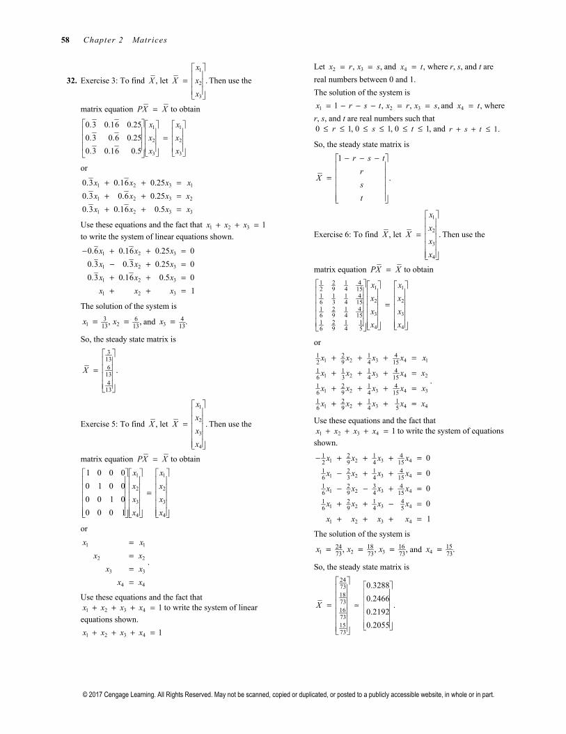
32. Exercise 3: To find ,X let

1

2

3

.

x

X x

x

=

Then use the

matrix equation PX X= to obtain

1 1

2 2

3 3

0.3 0.16 0.25

0.3 0.6 0.25

0.3 0.16 0.5

x x

x x

x x

=

or

1 2 3 1

1 2 3 2

1 2 3 3

0.3 0.16 0.25

0.3 0.6 0.25

0.3 0.16 0.5

x x x x

x x x x

x x x x

+ + =+ + =+ + =

Use these equations and the fact that 1 2 3 1x x x+ + =to write the system of linear equations shown.

1 2 3

1 2 3

1 2 3

1 2 3

0.6 0.16 0.25 0

0.3 0.3 0.25 0

0.3 0.16 0.5 0

1

x x x

x x x

x x x

x x x

− + + =− + =+ + =+ + =


1 23 6

13 13, ,x x= = and 3

413

.x =

So, the steady state matrix is

3136

134

13

.X

=

Exercise 5: To find ,X let

1

2

3

4

.

x

xX

x

x

=

Then use the


1 1

2 2

3 3

4 4

1 0 0 0

0 1 0 0

0 0 1 0

0 0 0 1

x x

x x

x x

x x

=

or

1 1

2 2

3 3

4 4

.

x x

x x

x x

x x

====

Use these equations and the fact that

1 2 3 4 1x x x x+ + + = to write the system of linear

equations shown.

1 2 3 4 1x x x x+ + + =

Let 2 3, ,x r x s= = and 4 ,x t= where r, s, and t are

real numbers between 0 and 1.


1 2 31 , , ,x r s t x r x s= − − − = = and 4 ,x t= where

r, s, and t are real numbers such that 0 1, 0 1, 0 1,r s t≤ ≤ ≤ ≤ ≤ ≤ and 1.r s t+ + ≤


1

.

r s t

rX

s

t

− − − =

Exercise 6: To find ,X let

1

2

3

4

.

x

xX

x

x

=

Then use the


1 1

2 2

3 3

4 4

1 2 1 42 9 4 151 1 1 46 3 4 151 2 1 46 9 4 151 2 1 16 9 4 5

x x

x x

x x

x x

=

or

1 2 3 4 1

1 2 3 4 2

1 2 3 4 3

1 2 3 4 4

1 2 1 42 9 4 151 1 1 46 3 4 151 2 1 46 9 4 151 2 1 16 9 4 5

x x x x x

x x x x x

x x x x x

x x x x x

+ + + =

+ + + =

+ + + =

+ + + =

.

Use these equations and the fact that

1 2 3 4 1x x x x+ + + = to write the system of equations

shown.

1 2 3 4

1 2 3 4

1 2 3 4

1 2 3 4

1 2 3 4

1 2 1 42 9 4 151 2 1 46 3 4 15

31 2 46 9 4 151 2 1 46 9 4 5

0

0

0

0

1

x x x x

x x x x

x x x x

x x x x

x x x x

− + + + =

− + + =

− − + =

+ + − =

+ + + =


1 2 318 1624

73 73 73, , ,x x x= = = and 4

1573

.x =


2473187316731573

0.3288

0.2466.

0.2192

0.2055

X

= ≈



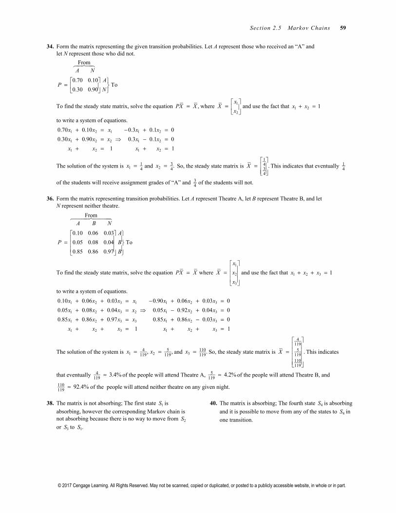
34. Form the matrix representing the given transition probabilities. Let A represent those who received an “A” and let N represent those who did not.

From

0.70 0.10To

0.30 0.90

A N

AP

N

=

To find the steady state matrix, solve the equation ,PX X= where 1

2

xX

x

=

and use the fact that 1 2 1x x+ =

to write a system of equations.

1 2 1 1 2

1 2 2 1 2

1 2 1 2

0.70 0.10 0.3 0.1 0

0.30 0.90 0.3 0.1 0

1 1

x x x x x

x x x x x

x x x x

+ = − + =+ = − =+ = + =


x = and 234.x = So, the steady state matrix is

1434

.X

=

This indicates that eventually 14

of the students will receive assignment grades of “A” and 34

of the students will not.

36. Form the matrix representing transition probabilities. Let A represent Theatre A, let B represent Theatre B, and let N represent neither theatre.

From

0.10 0.06 0.03

0.05 0.08 0.04 To

0.85 0.86 0.97

A B N

A

P B

B

=

To find the steady state matrix, solve the equation PX X= where

1

2

3

x

X x

x

=

and use the fact that 1 2 3 1x x x+ + =

to write a system of equations.

1 2 3 1 1 2 3

1 2 3 2 1 2 3

1 2 3 3 1 2 3

1 2 3 1 2 3

0.10 0.06 0.03 0.90 0.06 0.03 0

0.05 0.08 0.04 0.05 0.92 0.04 0

0.85 0.86 0.97 0.85 0.86 0.03 0

1 1

x x x x x x x

x x x x x x x

x x x x x x x

x x x x x x

+ + = − + + =+ + = − + =+ + = + − =+ + = + + =

The solution of the system is 1 254

119 119, ,x x= = and 3

110119

.x = So, the steady state matrix is

4119

5119110119

.X

=

This indicates

that eventually 4119

3.4%≈ of the people will attend Theatre A, 5119

4.2%≈ of the people will attend Theatre B, and

110119

92.4%≈ of the people will attend neither theatre on any given night.

38. The matrix is not absorbing; The first state 1S is

absorbing, however the corresponding Markov chain is not absorbing because there is no way to move from 2S

or 3S to 1.S

40. The matrix is absorbing; The fourth state 4S is absorbing

and it is possible to move from any of the states to 4S in

one transition.



42. Use the matrix equation ,PX X= or

1 1

2 2

3 3

0.1 0 0

0.2 1 0

0.7 0 1

x x

x x

x x

=

along with the equation 1 2 3 1x x x+ + = to write the

linear system

1

1

1

1 2 3

0.9 0

0.2 0.

0.7 0

1

x

x

x

x x x

− ===

+ + =

The solution of this system is 1 0,x = 2 1 ,x t= − and

3 ,x t= where t is a real number such that 0 1.t≤ ≤


0

1 ,X t

t

= −

where

0 1.t≤ ≤

44. Use the matrix equation PX X= or

1 1

2 2

3 3

4 4

0.7 0 0.2 0.1

0.1 1 0.5 0.6

0 0 0.2 0.2

0.2 0 0.1 0.1

x x

x x

x x

x x

=

along with the equation 1 2 3 4 1x x x x+ + + = to write

the linear system

1 3 4

1 3 4

3 4

1 3 4

1 2 3 4

0.3 0.2 0.1 0

0.1 0.5 0.6 0

.0.8 0.2 0

0.2 0.1 0.9 0

1

x x x

x x x

x x

x x x

x x x x

− + + =+ + =− + =+ − =

+ + + =

The solution of this system is 1 0,x = 2 1,x = 3 0,x =

and 4 0.x = So, the steady state matrix is

0

1.

0

0

X

=

46. Let nS be the state that Player 1 has n chips.

0 1 2 3 4

0

1

02

3

4

From

1 0.7 0 0 0 0

0 0 0.7 0 0 0

To and 0 0.3 0 0.7 0 1

0 0 0.3 0 0 0

0 0 0 0.3 1 0

S S S S S

S

S

P XS

S

S

= =

So,

0 0

4958

958

0

.0

0

nP X PX

→ =

So, the probability that Player 1 reaches 4S and wins the

tournament is 958

0.155.≈

48. (a) To find the nth state matrix of a Markov chain,

compute 0,nnX P X= where 0X is the initial state

matrix.

(b) To find the steady state matrix of a Markov chain,

determine the limit of 0,nP X as ,n → ∞ where 0X

is the initial state matrix.

(c) The regular Markov chain is 2 30 0 0, , , ,PX P X P X

where P is a regular stochastic matrix and 0X is the

initial state matrix.

(d) An absorbing Markov chain is a Markov chain with at least one absorbing state and it is possible for a member of the population to move from any nonabsorbing state to an absorbing state in a finite number of transitions.

(e) An absorbing Markov chain is concerned with having an entry of 1 and the rest 0 in a column, whereas a regular Markov chain is concerned with the repeated multiplication of the regular stochastic matrix.



50. (a) When the chain reaches 1S or 4 ,S it is certain in the

next step to transition to an adjacent state, 2S or 3,S

respectively, so 1S and 4S reflect to 2S or 3.S

(b) 0 0.4 0 0

1 0 0.3 0

0 0.6 0 1

0 0 0.7 0

P

=

(c)

30

30

1 16 6

5 512 12

5 56 6

7 712 12

1 16 6

5 56 12

5 56 6

7 712 12

0 0

0 0

0 0

0 0

0 0

0 0

0 0

0 0

P

P

≈

≈

Other high even or odd powers of P give similar results where the columns alternate.

(d)

1125245

12724

X

=

Half the sum entries in the corresponding columns of nP and 1nP + approach the corresponding entries in

.X

52. (a) Yes, it is possible.

(b) Yes, it is possible.

Both matrices X satisfy 1 .P X X= The steady state matrix depends on the initial state matrix. In general,

the steady state matrix is

6115 5

11 656

,

t

tX

t

t

−

− =

where t is any real number such that 611

0 .t≤ ≤ In

part (a) 0t = and in part (b), 611

.t =

54. Let

1 1

a bP

a b

= − −

be a 2 2× stochastic matrix, and consider the system of equations .PX X=

1 1

2 21 1

a b x x

a b x x

= − −

You have

( ) ( )1 2 1

1 2 21 1

ax bx x

a x b x x

+ =− + − =

or

( )( )

1 2

1 2

1 0

.1 0

a x bx

a x bx

− + =− − =

Letting 1x b= and 2 1 ,x a= − you have the 2 1× state

matrix X satisfying PX X=

.1

bX

a

= −

56. Let P be a regular stochastic matrix and 0X be the initial state matrix.

( )

( )

0 1 2

1 2

1 2

1 2

0

lim lim

lim lim lim

, where is a unique steady state matrix.

n nk

n n

n n nk

n n n

k

k

P X P x x x

P x P x P x

Px Px Px

P x x x

PX

X X

→∞ →∞

→∞ → ∞ →∞

= + + +

= ⋅ + ⋅ + + ⋅

= + + +

= + + +

=

=



Section 2.6 More Applications of Matrix Operations

2. Divide the message into groups of four and form the uncoded matrices.

[ ] [ ] [ ] [ ]H E L P _ I S _ C O M I N G _ _

8 5 12 16 0 9 19 0 3 15 13 9 14 7 0 0

Multiplying each uncoded row matrix on the right by A yields the coded row matrices

[ ] [ ]

[ ]

2 3 1 1

1 1 1 18 5 12 16 8 5 12 16

1 1 1 2

3 1 2 4

15 33 23 43

A

− − − − = − − − −

= − −

[ ] [ ][ ] [ ][ ] [ ]

0 9 19 0 28 10 28 47

3 15 13 9 7 20 7 2

14 7 0 0 35 49 7 7 .

A

A

A

= − −

= −

= − − −

So, the coded message is 15, 33, 23, 43, 28, 10,− − − − 28, 47, 7,− 20, 7, 2, 35,− 49, 7, 7.− −

4. Find 14 3

,3 2

A− − = −

and multiply each coded row matrix on the right by 1A− to find the associated uncoded row matrix.

[ ] [ ]

[ ] [ ][ ] [ ][ ] [ ][ ] [ ][ ] [ ][ ] [ ][ ] [ ][ ] [ ]

1

1

1

1

1

1

1

1

4 385 120 20 15 T,

3 2

6 8 0 2 _, B

10 15 5 0 E, _

84 117 15 18 O, R

42 56 0 14 _, N

90 125 15 20 O, T

60 80 0 20 _, T

30 45 15 0 O, _

19 26 2 5 B, E

O

A

A

A

A

A

A

A

A

−

−

−

−

−

−

−

−

− = −

=

=

=

=

=

=

=

=

So, the message is TO_BE_OR_NOT_TO_BE.

6. Find 1

11 2 8

4 1 3 ,

8 1 6

A−

− = − − −


[ ] [ ] [ ]1

11 2 8

112 140 83 112 140 83 4 1 3 8 1 22 H, A, V

8 1 6

A−

− − = − − = − −

[ ] [ ][ ] [ ][ ] [ ][ ] [ ][ ] [ ][ ] [ ]

1

1

1

1

1

1

19 25 13 5 0 1 E, _, A

72 76 61 0 7 18 _, G, R

95 118 71 5 1 20 E, A, T

20 21 38 0 23 5 _, W, E

35 23 36 5 11 5 E, K, E

42 48 32 14 4 0 N, D, _

A

A

A

A

A

A

−

−

−

−

−

−

− =

− =

− =

=

− =

− =

The message is HAVE_A_GREAT_WEEKEND_.

Section 2.6 More Applications of Matrix Operations 63


8. Let 1a b

Ac d

− =

and find that

[ ] [ ]

[ ] [ ]

_ S

19 19 0 19

U E

37 16 21 5 .

a b

c d

a b

c d

− − =

=

This produces a system of 4 equations.

19 19 0

19 19 19

37 16 21

37 16 5.

a c

b d

a c

b d

− − =− − =

+ =+ =

Solving this system, you find 1, 1, 1,a b c= = = − and

2.d = − So,

11 1

.1 2

A− = − −

Multiply each coded row matrix on the right by 1A− to yield the uncoded row matrices.

[ ] [ ] [ ] [ ] [ ][ ] [ ] [ ] [ ]3 1 , 14 3 , 5 12 , 0 15 , 18 4 ,

5 18 , 19 0 , 0 19 , 21 5 .

This corresponds to the message

CANCEL_ORDERS_SUE.

10. You have

[ ] [ ]45 35 10 15w x

y z

− =

and

[ ] [ ]38 30 8 14 .w x

y z

− =

So, 45 35 10

38 30 8

w y

w y

− =− =

and 45 35 15

38 30 14.

x z

x z

− =− =

Solving these two systems gives 1,w y= = 2,x = −

and 3.z = − So,

11 2

.1 3

A− − = −

(b) Decoding, you have:

[ ] [ ][ ] [ ][ ] [ ][ ] [ ][ ] [ ][ ] [ ][ ] [ ][ ] [ ][ ] [ ][ ] [ ]

1

1

1

1

1

1

1

1

1

1

45 35 10 15 J, O

38 30 8 14 H, N

18 18 0 18 _, R

35 30 5 20 E, T

81 60 21 18 U, R

42 28 14 0 N, _

75 55 20 15 T, O

2 2 0 2 _, B

22 21 1 19 A, S

15 10 5 0 E, _

A

A

A

A

A

A

A

A

A

A

−

−

−

−

−

−

−

−

−

−

− =

− =

− =

− =

− =

− =

− =

− =

− =

− =

The message is JOHN_RETURN_TO_BASE_.

12. Use the given information to find .D

User

A B

0.30 0.20 A

Supplier0.40 0.40 B

D

=

The equation X DX E= + may be rewritten in the form ( ) ,I D X E− = that is

0.7 0.2 10,000

.0.4 0.6 20,000

X−

= −

Solve this system by using Gauss-Jordan elimination to obtain

29,412

.52,941

x

≈



14. From the given matrix D, form the linear system ,X DX E= + which can be written as ( ) ,I D X E− =

that is

0.8 0.4 0.4 5000

0.4 0.8 0.2 2000 .

0 0.2 0.8 8000

X

− − − − = −

Solving this system,

21,875

17,000 .

14,250

X

=

16. (a) The line that best fits the given points is shown in the graph.

(b) Using the matrices

1 3

1 1

1 1

1 3

X

− − =

and

0

1,

1

2

Y

=

you have 4 0

,0 20

TX X

=

4,

6TX Y

=

and

( ) 114

311020

10 4.

0 6T TA X X X Y

− = = =

So, the least squares regression line is 310

1.y x= +

(c) Solving Y XA E= + for E, you have

0.1

0.3.

0.3

0.1

E Y XA

− = − = −

So, the sum of the squares error is 0.2.TE E =

18. (a) The line that best fits the given points is shown in the graph.

(b) Using the matrices

1 1

1 2

1 3

1 3

1 4

1 4

1 5

1 6

X

=

and

0

0

0

1,

1

2

2

2

Y

=

you have

8 28

,28 116

TX X

=

8,

37TX Y

=

and

( ) ( )13412

.T TA X X X Y− −

= =

So, the least squares regression line is 312 4

.y x= −

(c) Solving Y XA E= + for E, you have

3 31 1 1 1 1 14 4 4 4 4 4 4 4

TE Y XA = − = − − − −

and the sum of the squares error is 1.5.TE E =

20. Using the matrices

1 1

1 3

1 5

X

=

and

0

3 ,

6

Y

=

you have

( ) ( )13232

1 11 1 1 3 9

1 3 ,1 3 5 9 35

1 5

01 1 1 9

3 , and1 3 5 39

6

.

T

T

T T

X X

X Y

A X X X Y−

= =

= =

−= =

So, the least squares regression line is 3 32 2.y x= −

−1 1 2 3

2

−2

3

4

x

(3, 2)

(1, 1)(−1, 1)

(−3, 0)

y

5 6

2

1

−2

3

4

x

(4, 2)

(5, 2)

(6, 2)(4, 1)

(3, 1)(1, 0)

(3, 0)(2, 0)

y

Section 2.6 More Applications of Matrix Operations 65


22. Using matrices

1 4

1 2

1 2

1 4

X

− − =

and

1

0,

4

5

Y

− =

you have

4 0 8

, ,0 40 32

T TX X X Y

= =

and

( ) ( )114

140

0 8 2.

0 32 0.8T TA X X X Y

− = = =

So, the least squares regression line is 0.8 2.y x= +

24. Using matrices

1 3

1 1

1 1

1 3

X

− − =

and

4

2,

1

0

Y

=

you have

4 0

,0 20

TX X

=

7,

13TX Y

= −

and

( ) ( )171

4 4131

20 20

0 7.

0 13T TA X X X Y

− = = = −−

So, the least squares regression line is 0.65 1.75.y x= − +

26. Using matrices

1 0 6

1 4 3

and ,1 5 0

1 8 4

1 10 5

X Y

= = −

−

you have

1 0

1 41 1 1 1 1 5 27

,1 50 4 5 8 10 27 205

1 8

1 10

6

31 1 1 1 1 0

, and00 4 5 8 10 70

4

5

T

T

X X

X Y

= =

= = − − −

A = ( ) ( )1 1296

1296

205 27 0

27 5 70

1890.

350

T TX X X Y− −

= − −

= −

So, the least squares regression line is 175 945148 148.y x= − +

28. Using matrices

1 9 0.72

1 10 0.92

and ,1 11 1.17

1 12 1.34

1 13 1.60

X Y

= =

you have

5 55 5.75

and .55 615 65.43

T TX X X Y

= =

( ) 1 1.248

0.218T TA X X X Y

− − = =

So, the least squares regression line is 0.218 1.248.y x= −

30. (a) To encode a message, convert the message to numbers and partition it into uncoded row matrices of size 1 .n× Then multiply on the right by an invertible n n× matrix A to obtain coded row matrices. To decode a message,

multiply the coded row matrices on the right by 1A− and convert the numbers back to letters.

(b) A Leontief input-output model uses an n n× matrix to represent the input needs of an economic system, and an 1n × matrix to represent any external demands on the system.

(c) The coefficients of the least squares regression line are given by ( ) 1.T TA X X X Y

−=



Review Exercises for Chapter 2

2.

1 2 7 1 2 4 56 8 54 4

2 5 4 8 1 2 10 8 8 16 2 24

6 0 1 4 12 0 8 32 4 32

− − − − + = − + = − − −

4. ( ) ( ) ( ) ( ) ( ) ( )( ) ( ) ( ) ( ) ( ) ( )

1 6 5 4 1 2 5 0 1 8 5 01 5 6 2 8 26 2 8

2 6 4 4 2 2 4 0 2 8 4 02 4 4 0 0 4 4 16

+ − + +− − = = − − − −− − −

6. 2 1 4 2 2 4 5 5 2 4 3 9

6 0 3 1 0 4 24 12 0 4 24 16

− − + = + = −

8. Letting 1

2

2 1, ,

3 2

xA

x

− = =

x and 5

,4

= −

b the

system can be written as

1

2

2 1 5.

3 2 4

A

x

x

=

− = −

x b

Using Gaussian elimination, the solution of the system is 67

237

. = −

x

10. Letting

1

2

3

2 3 1 10

2 3 3 , , and 22 ,

4 2 3 2

x

A x

x

= − − = = − −

x b

the system can be written as

1

2

3

2 3 1 10

2 3 3 22 .

4 2 3 2

A

x

x

x

=

− − = − −

x b

Using Gaussian elimination, the solution of the system is 5

2 .

6

= −

x

12. 3 2

1 0

3 2 3 1 13 3

1 0 2 0 3 1

3 1 3 2 10 6

2 0 1 0 6 4

T

T

T

A

A A

AA

= −

− − = = − −

− = = −

14.

[ ]

[ ] [ ]

1

2

3

1 1 2 3

2 1 2 3 2 4 6

3 3 6 9

1

1 2 3 2 14

3

T

T

T

A

A A

AA

= − −

− − = − − − = − − −

= − − − = −

16. From the formula

1 1,

d bA

ad bc c a− −

= − −

you see that ( ) ( )( )4 2 1 8 0,ad bc− = − − − = and so the

matrix has no inverse.

18. Begin by adjoining the identity matrix to the given matrix.

[ ]1 1 1 1 0 0

0 1 1 0 1 0

0 0 1 0 0 1

A I

=

This matrix reduces to

1

1 0 0 1 1 0

0 1 0 0 1 1 .

0 0 1 0 0 1

I A−

− = −

So, the inverse matrix is

1

1 1 0

0 1 1 .

0 0 1

A−

− = −

Review Exercises for Chapter 2 67


20.

1

2

3 2 1

1 4 3

A

x

x

= −

x b

Because 12 15 51

10 3110 10

4 2,

1 3A−

−− = = −−

solve the

equation A =x b as follows.

12 15 5

3110 10

1 1

3 1A−

− = = = − − −

x b

22.

1

2

3

1 1 2 0

1 1 1 1

2 1 1 2

A

x

x

x

− = −

x b

Using Gauss-Jordan elimination, you find that

1

32 15 5 5

31 15 5 53 1 25 5 5

.A−

−

= − −

Solve the equation A =x b as follows.

1

32 15 5 5

31 15 5 53 1 25 5 5

0 1

1 1

2 1

A−

− = = − − = − −

x b

24.

2 1 5

3 4 2

A

x

y

− = −

x b

Because 14 1

11 11111 3 2

11 11

4 1,

3 2A−

= = −−

solve the

equation

Ax = b as follows.

1184 1

11 11 113 192

11 11 11

5

2A−

= − −−

x = b =

26.

0 1 2 0

3 2 1 1

4 3 4 7

A

x

y

z

= − − − −

x b

Using Gauss-Jordan elimination, you find that

1

5 1 118 9 68 4 19 9 3

17 2 118 9 6

A−

= − − −

Solve the equation Ax = b as follows.

1

5 231 118 9 6 188 174 19 9 3 9

17 172 118 9 6 18

0

1

7

A−

− − − − = − − −

x = b =

28. Because ( ) 1 2 42 ,

0 1A

− =

you can use the formula for

the inverse of a 2 2× matrix to obtain

1

2 4 1 4 1 41 12 .

2 0 20 1 0 2 0 2A

− − − = = = −

So,

111 41 4 .

4 0 2 10

2

A

− − = =

30. The matrix 2

1 4

x

will be nonsingular if

( )( ) ( )( )2 4 1 0,ad bc x− = − ≠ which implies that

8.x ≠

32. Because the given matrix represents 6 times the second

row, the inverse will be 16

times the second row.

16

1 0 0

0 0

0 0 1

For Exercises 34 and 36, answers will vary. Sample answers are shown below.

34. Begin by finding a sequence of elementary row operations to write A in reduced row-echelon form.


1 4

3 13

− −

Interchange the rows. 1

0 1

1 0E

=

1 4

0 1

−

Add 3 times row 1 to row 2. 2

1 0

3 1E

=

1 0

0 1

Add 4 times row 2 to row 1. 3

1 4

0 1E

=

Then, you can factor A as follows.

1 1 11 2 3

0 1 1 0 1 4

1 0 3 1 0 1A E E E− − − −

= = −



36. Begin by finding a sequence of elementary row operations to write A in reduced row-echelon form.


1 0 2

0 2 0

1 0 3

Multiply row one by 13. 1

13

0 0

0 1 0

0 0 1

E

=

1 0 2

0 2 0

0 0 1

Add 1− times row one to row three. 2

1 0 0

0 1 0

1 0 1

E

= −

1 0 0

0 2 0

0 0 1

Add 2− times row three to row one. 3

1 0 2

0 1 0

0 0 1

E

− =

1 0 0

0 1 0

0 0 1

Multiply row two by 12. 4

12

1 0 0

0 0

0 0 1

E

=

So, you can factor A as follows.

1 1 1 11 2 3 4

3 0 0 1 0 0 1 0 2 1 0 0

0 1 0 0 1 0 0 1 0 0 2 0

0 0 1 1 0 1 0 0 1 0 0 1

A E E E E− − − −

= =

38. Letting ,a b

Ac d

=

you have

2

22

0 0.

0 0

a b a b a bc ab bdA

c d c d ac dc cb d

+ + = = = + +

So, many answers are possible.

0 0 0 1

, , etc.0 0 0 0

40. There are many possible answers.

0 1

,0 0

A

=

1 0 0 1 1 0 0 00

0 0 0 0 0 0 0 0B AB

= = = =

But, 1 0 0 1 0 1

0.0 0 0 0 0 0

BA

= = ≠



42. Because ( )( )1 1 1 1 ,A B A B I− − − −+ + = if ( ) 11 1A B−− −+ exists, it is sufficient to show that ( ) ( )( )11 1A B A A B B I

−− −+ + =

for equality of the second factors in each equation.

( ) ( )( ) ( )( ) ( )( )( ) ( )

( ) ( )( ) ( )( )( ) ( )( )

( )( )( )( )

1 1 11 1 1 1

1 11 1

1 11

11

11 1

11

11

1

1

A B A A B B A A A B B B A A B B

A A A B B B A A B B

I A B B B A A B B

I B A A B B

B B B A A B B

B B A A B B

B A B A B B

B IB

B B

I

− − −− − − −

− −− −

− −−

−−

−− −

−−

−−

−

−

+ + = + + +

= + + +

= + + +

= + +

= + +

= + +

= + +

===

Therefore, ( ) ( )1 11 1 .A B A A B B− −− −+ = +


Matrix Elementary Matrix

1

3 1

12 0

3 1 1 0

0 4 4 1

1 0 3 1

4 1 0 4

A

U E

EA U

A E U LU−

− =

−

= = − =

− = = = −


1 1 1

1 2 2

1 2 3

1 1 1

0 1 1

1 2 3

1 1 1

0 1 1

0 1 2

1 1 1

0 1 1

0 0 1

A

U

=

=

1

2

3

1 0 0

1 1 0

0 0 1

1 0 0

0 1 0

1 0 1

1 0 0

0 1 0

0 1 1

E

E

E

= −

= −

= −

1 1 13 2 1 1 2 3

1 0 0 1 1 1

1 1 0 0 1 1

1 1 1 0 0 1

E E E A U A E E E U LU− − −

= = = =




2 1 1 1

0 3 1 1

0 0 2 0

2 1 1 2

A

− − = − −

2 1 1 1 1 0 0 0

0 3 1 1 0 1 0 0

0 0 2 0 0 0 1 0

0 0 0 1 1 0 0 0

U E

− − = = − − −

1 0 0 0 2 1 1 1

0 1 0 0 0 3 1 1

0 0 1 0 0 0 2 0

1 0 0 1 0 0 0 1

EA U A LU

− − = = = − −

1

2

3

4

1 0 0 0 7 7

0 1 0 0 3 3:

0 0 1 0 2 2

1 0 0 1 8 1

y

yL

y

y

− − = = =

y b y

1

2

3

4

2 1 1 1 7 4

0 3 1 1 3 1:

0 0 2 0 2 1

0 0 0 1 1 1

x

xU

x

x

− − − − = = − − − −

x = y x

50. 100 90 70 30 110 99 77 33

1.140 20 60 60 44 22 66 66

=

52. (a) In matrix B, grading system 1 counts each midterm as 25% of the grade and the final exam as 50% of the grade. Grading system 2 counts each midterm as 20% of

the grade and the final exam as 60% of the grade.

(b)

78 82 80 80 80

84 88 85 85.5 85.40.25 0.20

92 93 90 91.25 910.25 0.20

88 86 90 88.5 88.80.50 0.60

74 78 80 78 78.4

96 95 98 96.75 97

AB

= =

(c) Two students received an “A” in each grading system.

54. ( )3

2 1 2 1 1 03 2

1 0 1 0 0 1

4 3 6 3 2 0

3 2 3 0 0 2

0 0

0 0

f A

= − + − −

= − + − − −

=

56. The matrix is not stochastic because the sum of entries in columns 1 and 2 do not add up to 1.

58. This matrix is stochastic because each entry is between 0 and 1, and each column adds up to 1.

60. 1 0

2 1

3 2

0.307

0.693

0.38246

0.61754

0.3659

0.6341

X PX

X PX

X PX

= =

= =

= =

62. 1 0

2 1

3 2

495271027

378122812281

1032435924313

0.4

0.185

0.370

0.4568

0.2716

0.2716

0.4239

0.2428

0.3

X PX

X PX

X PX

= = ≈

= = ≈

= = ≈



64. Begin by forming the matrix of transition probabilities.

From Region

1 2 3

0.85 0.15 0.10 1

0.10 0.80 0.10 2 To Region

0.05 0.05 0.80 3

P

=

(a) The population in each region after 1 year is given by

131313

0.85 0.15 0.10 0.36

0.10 0.80 0.10 0.3 .

0.05 0.05 0.80 0.3

PX

= =

So,

0.36 110,000 Region 1

300,000 0.3 100,000 Region 2.

0.3 90,000 Region 3

=

(b) The population in each region after 3 years is given by

3

131313

0.665375 0.322375 0.2435 0.4104

0.219 0.562 0.219 0.3 .

0.115625 0.115625 0.5375 0.25625

P X

= =

So,

0.4104 123,125 Region 1

300,000 0.3 100,000 Region 2.

0.25625 76,875 Region 3

=


4737

1

0P

=

is not regular because nP has a zero in the first column for all powers.

To find ,X begin by letting 1

2

.x

Xx

=

Then use the


1 1

1 2

4737

1.

0

x x

x x

=

Use these matrices and the fact that 1 2 1x x+ = to write

the system of linear equations shown.

2

2

1 2

47

47

0

0

1

x

x

x x

=

− =

+ =

The solution of the system is 1 1x = and 2 0x =

So, the steady state matrix is 1

.0

X

=


0 0 0.2

0.5 0.9 0

0.5 0.1 0.8

P

=


To find ,X let [ ]1 2 3 .T

X x x x= Then use the matrix

equation PX X= to obtain.

1 1

2 2

3 3

0 0 0.2

0.5 0.9 0 .

0.5 0.1 0.8

x x

x x

x x

=

Use these matrices and the fact that 1 2 3 1x x x+ + = to

write the system of linear equations shown. 1 3

1 2

1 2 3

1 2 3

0.2 0

0.5 0.1 0

0.5 0.1 0.2 0

1

x x

x x

x x x

x x x

− + =− =+ − =+ + =


,x = 25

11,x = and

35

11.x =


1115

115

11

.X

=



70. Form the matrix representing the given probabilities. Let C represent the classified documents, D represent the declassified documents, and S represent the shredded documents.

From

0.70 0.20 0

0.10 0.75 0 To

0.20 0.05 1

C D S

C

P D

S

=

Solve the equation ,PX X= where

1

2

3

x

X x

x

=

and use the fact that 1 2 3 1x x x+ + = to write a system of equations.

1 2 1 1 2

1 2 2 1 2

1 2 3 3 1 2

1 2 3 1 2 3

0.70 0.20 0.3 0.2 0

0.10 0.75 0.1 0.25 0

0.20 0.05 0.2 0.05 0

1 0

x x x x x

x x x x x

x x x x x x

x x x x x x

+ = − + =+ = − =+ + = + =+ + = + + =


0

0 .

1

X

=

This indicates that eventually all of the documents will be shredded.

72. The matrix

1 0 0.38

0 0.30 0

0 0.70 0.62

P

=

is absorbing. The first state 1S is absorbing and it is possible to move from 2S to 1S in two transitions and to move from 3S to

1S in one transition.

74. (a) False. See Exercise 65, page 61.

(b) False. Let 1 0

0 1A

=

and 1 0

.0 1

B−

= −

Then 0 0

.0 0

A B

+ =

A B+ is a singular matrix, while both A and B are nonsingular matrices.

76. (a) True. See Section 2.5, Example 4(b).

(b) False. See Section 2.5, Example 7(a).

78. The uncoded row matrices are

[ ] [ ] [ ] [ ] [ ] [ ]B E A M _ M E _ U P _ S C O T T Y _

2 5 1 13 0 13 5 0 21 16 0 19 3 15 20 20 25 0

Multiplying each 1 3× matrix on the right by A yields the coded row matrices.

[ ] [ ] [ ] [ ] [ ] [ ]17 6 20 0 0 13 32 16 43 6 3 7 11 2 3 115 45 155− − − − − − −

So, the coded message is

17, 6, 20, 0, 0, 13, 32, 16, 43, 6, 3, 7, 11, 2, 3, 115, 45, 155.− − − − − − −



80. Find 1A− to be

13 4

1 1A− − −

=

and the coded row matrices are

[ ] [ ] [ ] [ ] [ ] [ ] [ ] [ ] [ ]11 52 , 8 9 , 13 39 , 5 20 , 12 56 , 5 20 , 2 7 , 9 41 , 25 100 .− − − − −

Multiplying each coded row matrix on the right by 1A− yields the uncoded row matrices.

[ ] [ ] [ ] [ ] [ ] [ ] [ ] [ ] [ ]S H O W _ M E _ T H E _ M O N E Y _

19 8 15 23 0 13 5 0 20 8 5 0 13 15 14 5 25 0

So, the message is SHOW_ME_THE_MONEY_.

82. Find 1A− to be

1

4 2 113 13 138 9 2

13 13 135 4 2

13 13 13

,A−

= − − −


[ ] [ ] [ ]1

4 2 113 13 138 9 2

13 13 135 4 2

13 13 13

66 27 31 66 27 31 25 1 14 Y, A, NA−

− = − − = − −

[ ] [ ][ ] [ ][ ] [ ][ ] [ ][ ] [ ][ ] [ ][ ] [ ]

1

1

1

1

1

1

1

37 5 9 11 5 5 K, E, E

61 46 73 19 0 23 S, _, W

46 14 9 9 14 0 I, N, _

94 21 49 23 15 18 W, O, R

32 4 12 12 4 0 L, D, _

66 31 53 19 5 18 S, E, R

47 33 67 9 5 19 I, E, S

A

A

A

A

A

A

A

−

−

−

−

−

−

−

− =

− =

− =

− =

− =

− =

− =

[ ] [ ][ ] [ ][ ] [ ]

1

1

1

32 19 56 0 9 14 _, I, N

43 9 20 0 19 5 _, S, E

68 23 34 22 5 14 V, E, N

A

A

A

−

−

−

− =

− − =

− =

The message is YANKEES_WIN_WORLD_SERIES_IN_SEVEN.

84. Solve the equation X DX E= + for X to obtain

( ) ,I D X E− = which corresponds to solving the

augmented matrix.

0.9 0.3 0.2 3000

0 0.8 0.3 3500

0.4 0.1 0.9 8500

− − − − −

The solution to this system is

10,000

10,000 .

15,000

X

=


1 2

1 3

1 4

1 5

1 6

X

=

and

1

3

,2

4

4

Y

=

you have

5 20

,20 90

TX X

=

14, and

63TX Y

=

( ) 1 1.8 0.4 14 0.

0.4 0.1 63 0.7T TA X X X Y

− − = = = −

So, the least squares regression line is 0.7 .y x=




1 2

1 1

1 0

1 1

1 2

X

− − =

and

4

2

,1

2

3

Y

= − −

you have

5 0

,0 10

TX X

=

2, and

18TX Y

= −

( ) 115

110

0 2 0.4.

18 1.80T TA X X X Y

− = = − −

So, the least squares regression line is 1.8 0.4,y x= − + or 9 25 5.y x= − +

90. (a) Using the matrices

1 8 2.93

1 9 3.00

1 10 3.01and , you have

1 11 3.10

1 12 3.21

1 13 3.39

X Y

= =

1 8

1 9

1 1 1 1 1 1 1 10 6 63

8 9 10 11 12 13 1 11 63 679

1 12

1 13

TX X

= =

and

2.93

3.00

1 1 1 1 1 1 3.01 18.64.

8 9 10 11 12 13 3.10 197.23

3.21

3.39

TX Y

= =

Now, using ( ) 1TX X−

to find the coefficient matrix A, you have

( ) 1397

15 5

3 25 35

18.64 2.2007.

197.23 0.0863T TA X X X Y

−−

−

= = ≈

So, the least squares regression line is 0.0863 2.2007.y x= +

(b) Using a graphing utility, the regression line is 0.0863 2.2007.y x= +

(c)

The estimated values are close to the actual values.

Year 2008 2009 2009 2010 2011 2012 2013

Actual 2.93 2.93 3.00 3.01 3.10 3.21 3.39

Estimated 2.89 2.89 2.98 3.06 3.15 3.24 3.32

Project Solutions for Chapter 2 75


Project Solutions for Chapter 2

1 Exploring Matrix Multiplication

1. Test 1 seems to be the more difficult test. The averages were:

Test 1 average 75

Test 2 average 85.5

==

2. Anna, David, Chris, Bruce


1

0M

represents scores on the first test.

0

1M

represents scores on the second test.


[ ]1 0 0 0 M represents Anna’s scores.

[ ]0 0 1 0 M represents Chris’s scores.


1

1M

represents the sum of the test scores for each

student, and 12

1

1M

represents each students’ average.

6. [ ]1 1 1 1 M represents the sum of scores on each test;

[ ]14

1 1 1 1 M represents the average on each test.

7. [ ] 11 1 1 1

1M

represents the overall points total for

all students on all tests.

8. [ ]18

11 1 1 1 80.25

1M

=

9. 1.1

1.0M

2 Nilpotent Matrices

1. 2 0A ≠ and 3 0,A = so the index is 3.

2. (a) Nilpotent of index 2

(b) Not nilpotent

(c) Nilpotent of index 2

(d) Not nilpotent

(e) Nilpotent of index 2

(f) Nilpotent of index 3

3.

0 0 1

0 0 0

0 0 0

index 2;

0 1 1

0 0 1

0 0 0

index 3

4.

0 0 0 1

0 0 0 0

0 0 0 0

0 0 0 0

index 2;

0 0 1 1

0 0 0 1

0 0 0 0

0 0 0 0

index 3;

0 1 1 1

0 0 1 1

0 0 0 1

0 0 0 0

index 4

5.

0 1 1 1 1

0 0 1 1 1

0 0 0 1 1

0 0 0 0 1

0 0 0 0 0

6. No. If A is nilpotent and invertible, then kA O= for

some k and 1 .kA O− ≠ So,

( )1 1 1 1 1 ,k k kA A I O A A A A A IA O− − − − −= = = = ≠

which is impossible.

7. If A is nilpotent, then ( ) ( ) .T kk TA A O= = But

( ) ( )1 1 ,k TT kA A O

− −= ≠ which shows that TA is

nilpotent with the same index.

8. Let A be nilpotent of index k. Then

( )( )1 2 2 ,k k kI A A A A A I I A I− −− + + + + + = − =

which shows that

( )1 2 2k kA A A A I− −+ + + + +

is the inverse of .I A−

Date post:	28-Aug-2018
Category:	Documents
Upload:	haque
View:	234 times
Download:	3 times

CHAPTER 2 Matrices - testbanklive.com · Section 2.4 Elementary Matrices ... Project Solutions ......

Documents