Chapter 2 Previous Work on Image Segmentationstrider/publications/Chapter2.pdf · Chapter 2...

Chapter 2

Previous Work on Image Segmentation

As described in the previous chapter, the image segmentation problem can be stated as the

division of an image into regions that separate different objects from each other, and from the

background. This chapter will review many of the existing segmentation techniques, it will

examine the principles behind them, and discuss the particular characteristics of each class of

algorithms. The purpose of this chapter is to give the reader an overview of the current state-of-

the-art in image segmentation, and, together with the review chapter on perceptual grouping,

to provide a background against which the contributions of our research can be weighted.

However, before undertaking a review of image segmentation techniques, it is important to be

more precise about the definition of the problem we are interested in.

As we mentioned in the previous chapter, we are interested in the problem of segmenting

a single image in a completely bottom-up fashion, that is, without prior knowledge of what

specific objects will be found in the scene. This means that the segmentation algorithms can

not use intensity, colour, texture, or feature descriptors that are specific to a known object, or

object class to produce the segmentation. Even though the use of prior knowledge about objects

can lead to algorithms that are successful in constrained environments, a general segmentation

technique is unlikely to use anything more specific than weak priors on the expected shapes of

objects (such as, for example, a preference for smooth boundaries, compact shapes, or simple

5

CHAPTER 2. PREVIOUS WORK ON IMAGE SEGMENTATION 6

contours).

It is also important to consider that the result of a bottom-up Image Segmentation procedure

is expected to be only an intermediate step, intended to reduce the complexity of processing that

higher levels need to carry out to produce some interpretation of the image. At best, bottom-up

segmentation can be expected to yield a few interesting regions that are likely to correspond to

objects of interest (or parts thereof) within the image.

The process of segmentation is directly tied to recognition, and it is likely that to achieve a

complete separation of objects from background, information that can only be obtained from

higher level recognition, inference, and perceptual completion procedures will be required.

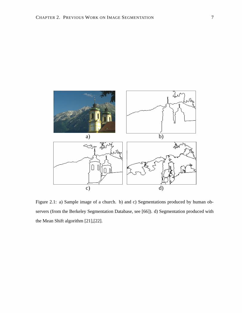
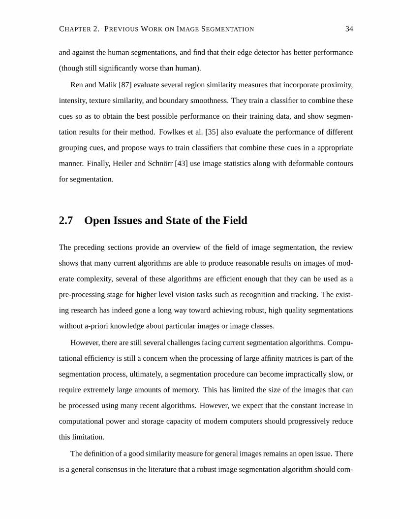
As an example of this, consider Figure 2.1. Human observers have no trouble segmenting

the image, but notice that they disagree about the level of detail at which the segmentation is to

be produced. One observer, for example, considers the towers as single entities, and disregards

areas of different color, while the other observer identifies the windows and top of the tower as

separate entities, but disregards the yellow areas of the walls as surface markings.

A bottom-up procedure has no such knowledge, and hence, should not be expected to pro-

duce segmentations in which every region is directly interpretable as a single object. Instead,

anything that looks reasonably different than its surroundings will be treated as a separate re-

gion, including surface markings, strong illumination effects such as highlights, and different

looking subparts of objects.

So how are we to evaluate the performance of a given segmentation algorithm? As of the

writing of this thesis, there was no universally accepted testing methodology or benchmarking

procedure. Some researchers argue that segmentation algorithms should be evaluated in the

context of a particular task, such as object recognition [9], that is, different algorithms should

be compared in terms of the potential benefit they provide for a particular higher-level task.

Other researchers (see for example [66]) propose that segmentation algorithms should be eval-

uated as stand-alone modules, by comparing their output to ’ground truth’ which is usually a

segmentation produced by human observers.


a)

c) d)

b)

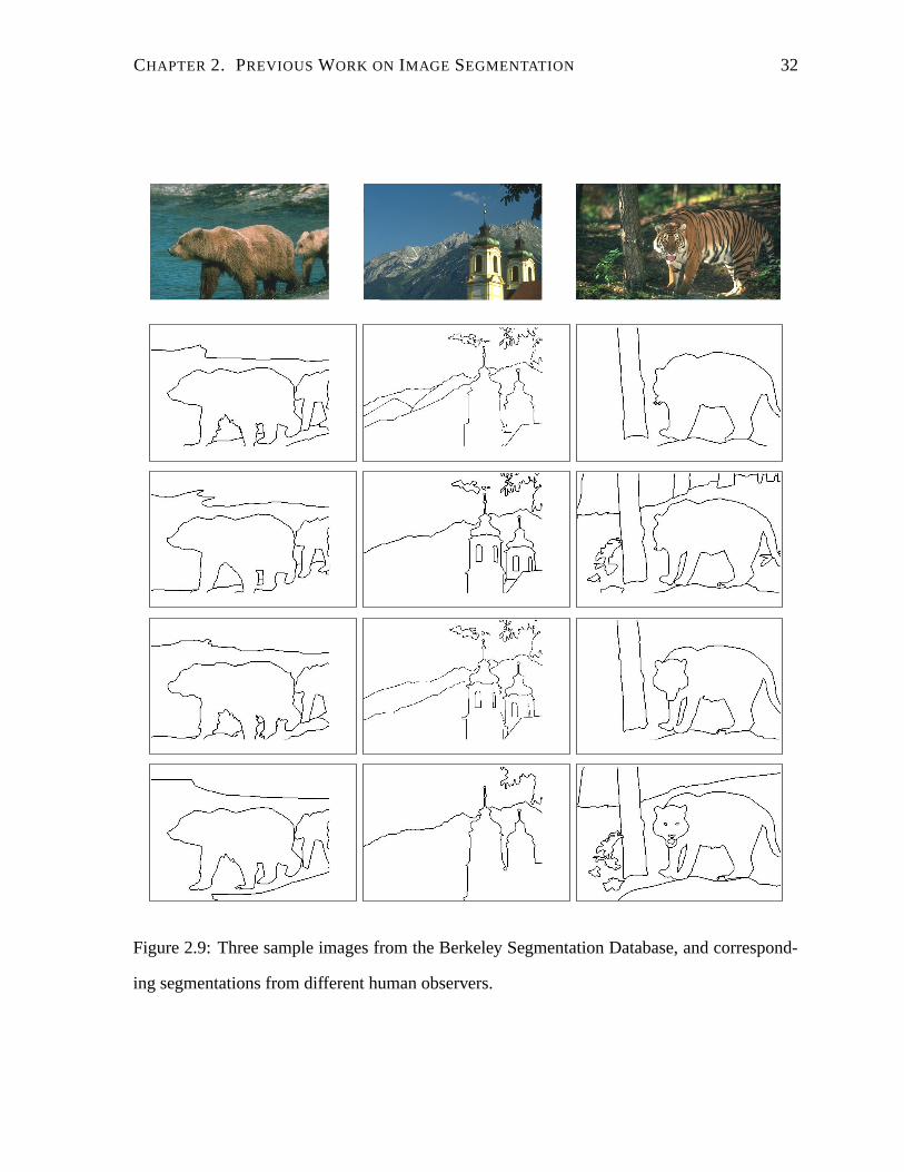
Figure 2.1: a) Sample image of a church. b) and c) Segmentations produced by human ob-

servers (from the Berkeley Segmentation Database, see [66]). d) Segmentation produced with

the Mean Shift algorithm [21],[22].


This latter view is more suitable for our purposes so for the remainder of the chapter,

experimental results are considered in the light of what a human observer would see in a given

image. This leads us to two essential problems: 1) Different human observers will produce

different segmentations of the same image, and 2) Human observers use high level knowledge,

and solve high level vision problems such as recognition and perceptual completion while

segmenting the image.

Recent research by Martin et al. [66] indicates that human segmentations do not vary ran-

domly, instead they show regularities that can be exploited to design and evaluate segmenta-

tion algorithms. It also suggests ways in which the use of higher level knowledge by human

observers can be accounted for, thus allowing for the direct comparison of segmentations pro-

duced by human observers and segmentation algorithms. These topics will be discussed at

length further on in this chapter.

With the above considerations in mind, bottom-up Image Segmentation can be formulated

as the problem of defining a similarity measure between image elements that can be evaluated

using image data, and the development of an algorithm that will group similar image elements

into connected regions, according to some grouping criterion. The image elements can be

pixels, small local neighborhoods, or image regions produced by an earlier stage of processing,

or by a previous step of an iterative segmentation procedure. The similarity function can use

one or many of the available image cues (such as image intensity, colour, texture, and various

filter responses), or be defined as a proximity measure on a suitable feature space that captures

interesting image structure. The two aspects of the segmentation task can be (and often have

been) studied separately, and through this review, it will be useful to remember the distinction

between the grouping procedure and the similarity measure used by a particular method. A

grouping procedure that does not depend on the particular form of the similarity measure is

likely to be applicable to a wider class of images.

From this point onward, we will use the term Image Segmentation, or simply ’segmenta-

tion’ to stand for bottom-up Image Segmentation as described above. Given the volume of


existing research, a complete survey including every existing technique is not practical. For

this reason, this chapter will only look at those algorithms that are most relevant to our re-

search effort. These algorithms have been roughly divided into the following classes: Early

region growing/splitting techniques, feature space methods, graph theoretic methods, spectral

segmentation techniques, deformable contours, and algorithms based on image statistics.

2.1 Early Segmentation Techniques

It is perhaps not surprising that the earliest segmentation techniques were based on gray-level

similarity. These algorithms were designed to locate simple objects, which could be assumed

to project to reasonably uniform image regions in terms of image intensity. The task of the

algorithm would be to identify contiguous pixels with similar gray-level value, and group them

into regions.

Several classifications have been proposed for algorithms that are based on gray-level pixel

similarity, and the number of existing variations of these methods number well into the hun-

dreds. Comprehensive reviews of early segmentation techniques can be found in [42], and [80].

Here we will discuss two broad classes of segmentation methods: Gray level thresholding, and

region growing/merging techniques.

Gray level thresholding is a generalization of binary thresholding [44]. Binary thresholding

works by determining the gray level value that separates pixels in the foreground from pixels

in the background, and generating a ’thresholded image’ where pixels are assigned one of two

possible values corresponding to ’foreground’ and ’background’ depending on whether their

gray level is above or below the selected threshold. Usually, the threshold level is determined

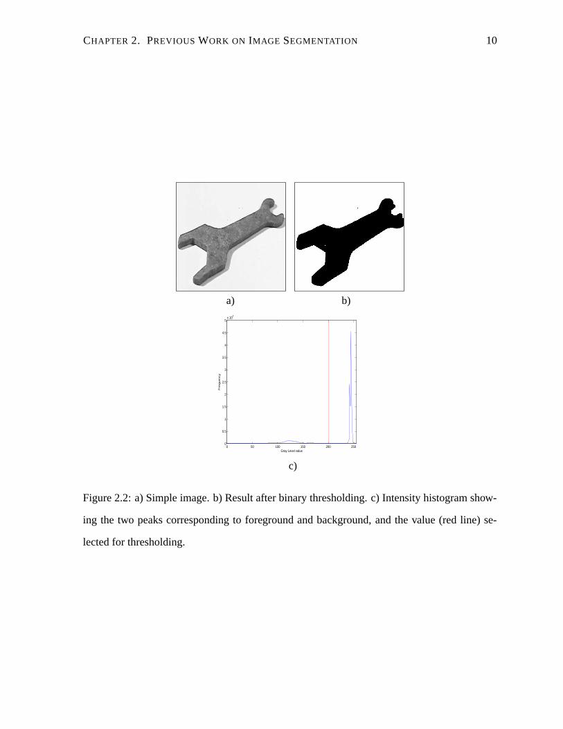
by examining the intensity histogram for the image. If the foreground and background are

simple and well differentiated, the histogram will show two large peaks corresponding to the

dominant gray value in each region. The threshold level corresponds to the minimum point at

the valley dividing the two peaks in the histogram. This is illustrated in Figure 2.2.


0 50 100 150 200 2500

0.5

1

1.5

2

2.5

3

3.5

4

4.5

5x 10

4

Gray Level value

Fre

qu

en

cy

b)

c)

a)

Figure 2.2: a) Simple image. b) Result after binary thresholding. c) Intensity histogram show-

ing the two peaks corresponding to foreground and background, and the value (red line) se-

lected for thresholding.


b)

c)

a)

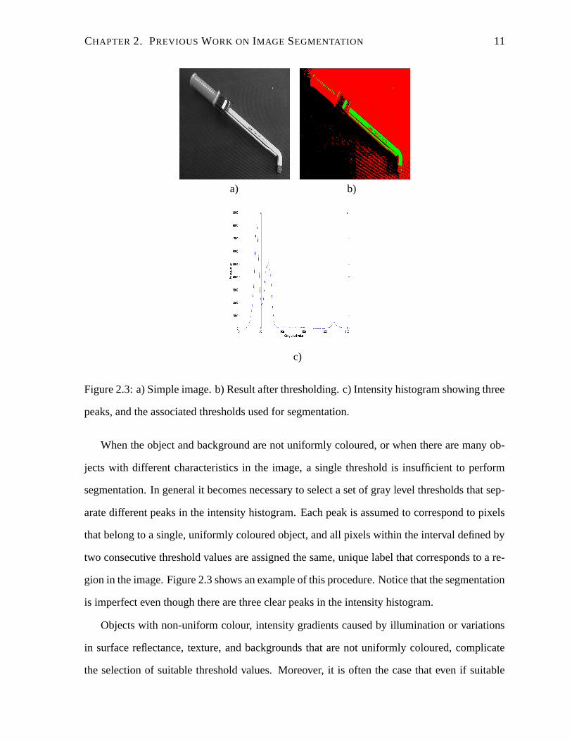
Figure 2.3: a) Simple image. b) Result after thresholding. c) Intensity histogram showing three

peaks, and the associated thresholds used for segmentation.

When the object and background are not uniformly coloured, or when there are many ob-

jects with different characteristics in the image, a single threshold is insufficient to perform

segmentation. In general it becomes necessary to select a set of gray level thresholds that sep-

arate different peaks in the intensity histogram. Each peak is assumed to correspond to pixels

that belong to a single, uniformly coloured object, and all pixels within the interval defined by

two consecutive threshold values are assigned the same, unique label that corresponds to a re-

gion in the image. Figure 2.3 shows an example of this procedure. Notice that the segmentation

is imperfect even though there are three clear peaks in the intensity histogram.

Objects with non-uniform colour, intensity gradients caused by illumination or variations

in surface reflectance, texture, and backgrounds that are not uniformly coloured, complicate

the selection of suitable threshold values. Moreover, it is often the case that even if suitable


values can be found, the resulting segmentation is inaccurate because of overlap in gray-level

intensities between different elements of the image, which leads to disconnected regions with

the same label. In complicated images, it also becomes difficult to separate different peaks in

the histogram, and to determine how many thresholds are required.

This leads to an important problem faced by all image segmentation algorithms: In the ab-

sence of prior knowledge about the image’s contents, it is in general not possible to determine

how many regions are required for a reasonable segmentation. This problem manifests itself

in two forms: Under-segmentation, which occurs when parts of the image that actually corre-

spond to different objects, or to an object and the background, are assigned to the same region;

and over-segmentation, which occurs when parts of the image corresponding to a single object

are split apart. Under-segmentation is considered the most serious of these problems, as it in-

volves the failure to detect a perceptually important boundary. Additionally, over-segmented

images can be improved using reasonably simple region merging procedures, while correctly

partitioning under-segmented images is a difficult problem. In general, a reasonable level of

over-segmentation can be expected, and is perhaps unavoidable given the nature of the seg-

mentation problem.

The second class of the early segmentation algorithms mentioned above starts with a set

of seed regions (individual pixels at the start of the procedure), and produces a segmentation

by iteratively merging together regions that are similar enough. There are many algorithms for

growing the regions, as well as for evaluating similarity between neighboring elements [42],

but the fundamental principle is the same: Each initial region will grow until no more similar

elements can be added to it. When none of the regions in the image can grow any more the

segmentation process is complete.

The work of Beveridge et al. [6] offers a good example of a procedure that integrates both

gray level thresholding and region merging. In their paper, an input image (which can be

either grayscale or colour) is divided into sectors of fixed size and fixed location. An intensity

histogram is calculated for each sector (and on colour images, for each colour channel), and


used to produce a local segmentation. For every sector, information from its neighbors is used

to detect clusters for which there may not be enough local support due to the artificially induced

partition of the image.

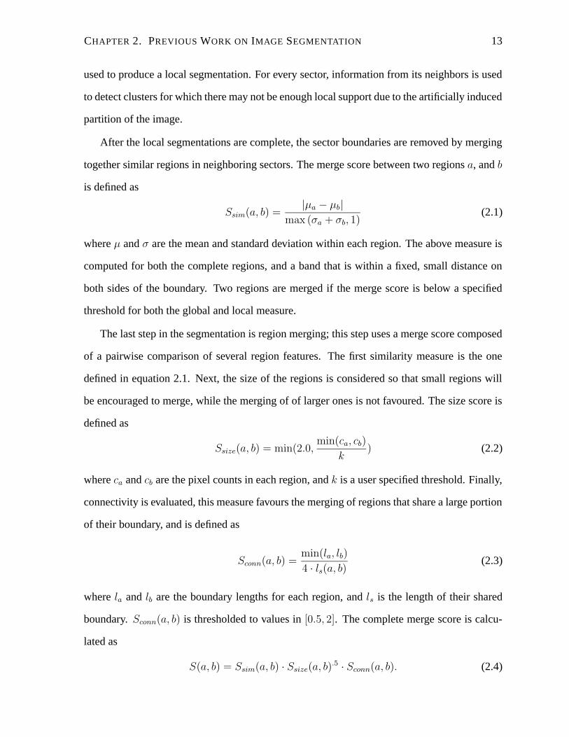
After the local segmentations are complete, the sector boundaries are removed by merging

together similar regions in neighboring sectors. The merge score between two regions a, and b

is defined as

Ssim(a, b) =|µa − µb|

max (σa + σb, 1)(2.1)

where µ and σ are the mean and standard deviation within each region. The above measure is

computed for both the complete regions, and a band that is within a fixed, small distance on

both sides of the boundary. Two regions are merged if the merge score is below a specified

threshold for both the global and local measure.

The last step in the segmentation is region merging; this step uses a merge score composed

of a pairwise comparison of several region features. The first similarity measure is the one

defined in equation 2.1. Next, the size of the regions is considered so that small regions will

be encouraged to merge, while the merging of of larger ones is not favoured. The size score is

defined as

Ssize(a, b) = min(2.0,min(ca, cb)

k) (2.2)

where ca and cb are the pixel counts in each region, and k is a user specified threshold. Finally,

connectivity is evaluated, this measure favours the merging of regions that share a large portion

of their boundary, and is defined as

Sconn(a, b) =min(la, lb)

4 · ls(a, b)(2.3)

where la and lb are the boundary lengths for each region, and ls is the length of their shared

boundary. Sconn(a, b) is thresholded to values in [0.5, 2]. The complete merge score is calcu-

lated as

S(a, b) = Ssim(a, b) · Ssize(a, b).5 · Sconn(a, b). (2.4)


Values of S(a, b) < 1 indicate a preference toward merging, if S(a, b) = 1 there is no prefer-

ence, and merging is discouraged if S(a, b) > 1. This process is repeated iteratively until no

further merging is possible.

Since the algorithm can only merge regions, the thresholds used during the local, thresh-

old based segmentation stage are selected so that they’ll yield a significantly over-segmented

image; the merging step is then relied upon to turn the unsegmented image into a reasonable

segmentation. Results presented in [6] show that this algorithm produces good segmentations

in parts of the image that are reasonably homogeneous, and over-segmented regions when there

is texture, significant intensity gradients, or objects with non-uniform coloring. The algorithm

is not without problems, as there are several thresholds that must be chosen carefully depend-

ing on the image, and the region boundaries themselves have slight artifacts introduced by the

sector-based initial segmentation. Even so, the algorithm illustrates what can be achieved with

thresholding/merging schemes.

2.2 Feature Space Analysis

In the previous section the histogram of gray-level intensities was used directly to determine

pixel categories within the image. Histogram analysis can be considered a special case of

feature space analysis. In general, each point in a data set (for our purposes, each pixel in

an image, though this can be generalized to pixel neighborhoods) is associated with a feature

vector that encodes some important characteristic of that particular point. In colour images, for

example, we can represent a pixel with a 3D vector that contains the RGB values of that pixel’s

colour. The feature vector itself can represent any of a number of image cues: colour, texture,

filter responses, spatial location, and so on. The space that contains these feature vectors is

what we call the feature space

For segmentation purposes, feature vectors are used to encode some image cue whose simi-

larity we wish to use as the basis of the segmentation process. It is expected that feature vectors


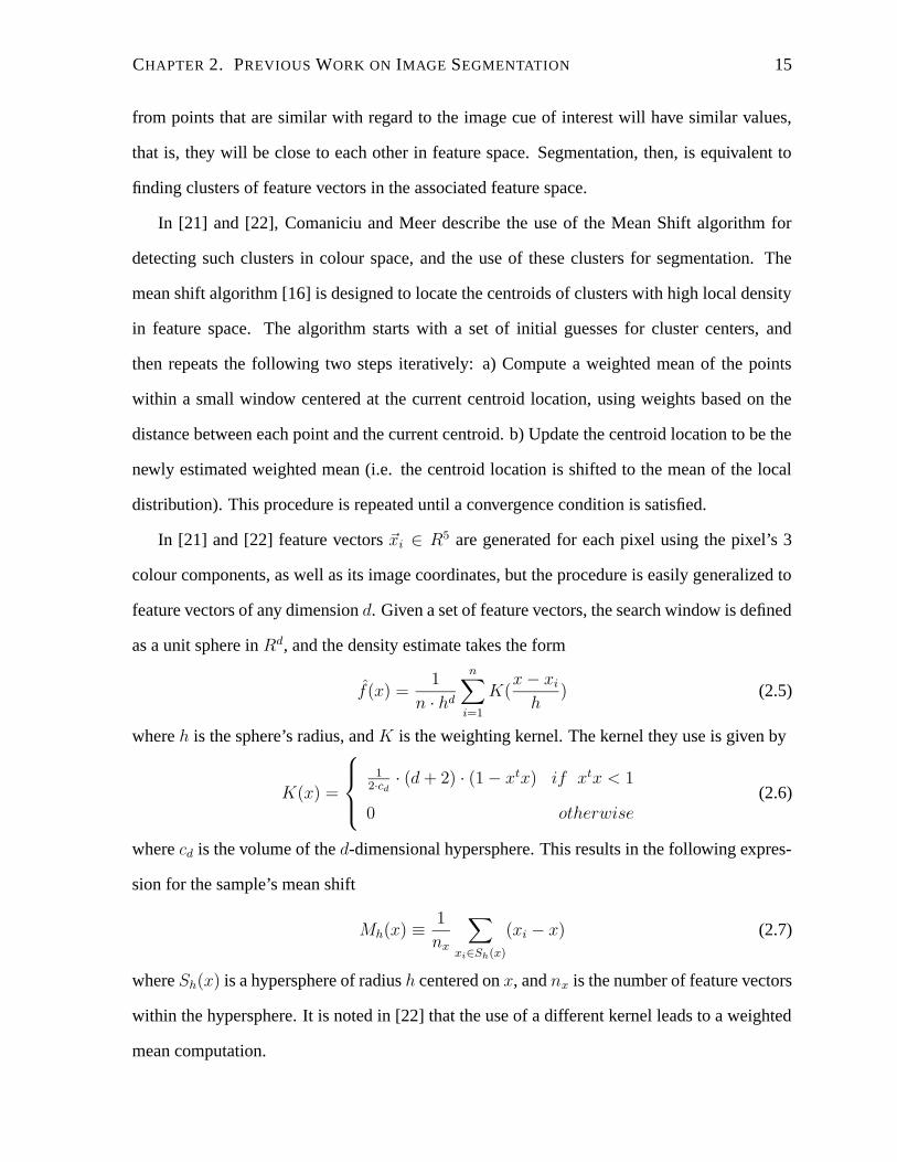
from points that are similar with regard to the image cue of interest will have similar values,

that is, they will be close to each other in feature space. Segmentation, then, is equivalent to

finding clusters of feature vectors in the associated feature space.

In [21] and [22], Comaniciu and Meer describe the use of the Mean Shift algorithm for

detecting such clusters in colour space, and the use of these clusters for segmentation. The

mean shift algorithm [16] is designed to locate the centroids of clusters with high local density

in feature space. The algorithm starts with a set of initial guesses for cluster centers, and

then repeats the following two steps iteratively: a) Compute a weighted mean of the points

within a small window centered at the current centroid location, using weights based on the

distance between each point and the current centroid. b) Update the centroid location to be the

newly estimated weighted mean (i.e. the centroid location is shifted to the mean of the local

distribution). This procedure is repeated until a convergence condition is satisfied.

In [21] and [22] feature vectors ~xi ∈ R5 are generated for each pixel using the pixel’s 3

colour components, as well as its image coordinates, but the procedure is easily generalized to

feature vectors of any dimension d. Given a set of feature vectors, the search window is defined

as a unit sphere in Rd, and the density estimate takes the form

f(x) =1

n · hd

n∑

i=1

K(x − xi

h) (2.5)

where h is the sphere’s radius, and K is the weighting kernel. The kernel they use is given by

K(x) =

12·cd

· (d + 2) · (1 − xtx) if xtx < 1

0 otherwise(2.6)

where cd is the volume of the d-dimensional hypersphere. This results in the following expres-

sion for the sample’s mean shift

Mh(x) ≡1

nx

∑

xi∈Sh(x)

(xi − x) (2.7)

where Sh(x) is a hypersphere of radius h centered on x, and nx is the number of feature vectors

within the hypersphere. It is noted in [22] that the use of a different kernel leads to a weighted

mean computation.


a) b) c)

Figure 2.4: a) Original image (640 × 480 pixels) . b) Mean-shift segmentation (coarse) c)

Mean-shift segmentation (fine). Run time for both segmentations was around 2.5 min. on a P4,

1.9 GHz. machine.

The above procedure will converge from an initial estimate to a region of locally maximal

density in feature space. The set of points of convergence for the input vectors corresponds to

the centroids of clusters in feature space that originate from groups of similar pixels, located

within a compact image neighborhood. For segmentation purposes, each pixel’s intensity or

color value is set to that of the corresponding point of convergence that signals the centroid

of a cluster. Cluster centers that are near enough are fused together, and regions smaller than

a user defined threshold are eliminated. Sample segmentations produced using the mean shift

algorithm are shown in Figure 2.4. These segmentations were generated using the EDISON

system [37] which implements the algorithms described in [21] and [22].

The mean-shift algorithm produces reasonable segmentations at coarser levels. However,

there is also noticeable over-segmentation. While the implementation used to generate Fig-

ure 2.4 uses only colour information to determine pixel similarity, it is possible in principle to

apply the same algorithm to feature vectors that contain texture descriptors and other image

cues.


2.3 Graph Theoretic Algorithms

There are several classes of algorithms that represent images as graphs, and then apply graph-

theoretic techniques to partition the graph into clusters that represent separate regions in the

image. Though several partitioning techniques exist, they all use the same underlying repre-

sentation of the image: a graph G(V,E) is constructed in which V is a set of vertices corre-

sponding to image elements (which may be pixels, feature descriptors, and so on), and E is a

set of edges linking vertices in the graph together. The weight of an edge wi,j is proportional

to the similarity between the vertices vi and vj and is usually referred to as the affinity between

elements i and j in the image.

The affinity value can use any of a number of image cues, including gray level intensity,

colour, texture, and other image statistics. It is also common to add a distance term that ensures

that the graph is sparse by linking together only those nodes that correspond to elements in the

image that are near each other. Once the graph is built, segmentation consists on determining

which subsets of nodes and edges that correspond to homogeneous regions in the image. The

key principle here is that nodes that belong to the same region or cluster should be joined by

edges with large weights, while nodes that are joined by weak edges are likely to belong to

different regions.

In [116], Wu and Leahy propose that image segmentation can be carried out by finding the

minimum cut through the graph, a cut through a graph defines the total weight of a set of links

that must be cut (removed) to divide the graph into two separate components

cut(A,B) =∑

i∈A,j∈B

wi,j (2.8)

MinCut(A,B) = min(cut(A,B)) (2.9)

where the minimum value is taken over all possible partitions of the graph into two components.

Intuitively, the minimum-cut corresponds to finding the subset of edges of least weight that can

be removed to partition the image in two. Since edges encode similarity, this is equivalent to

splitting the image along the boundary of least similarity.


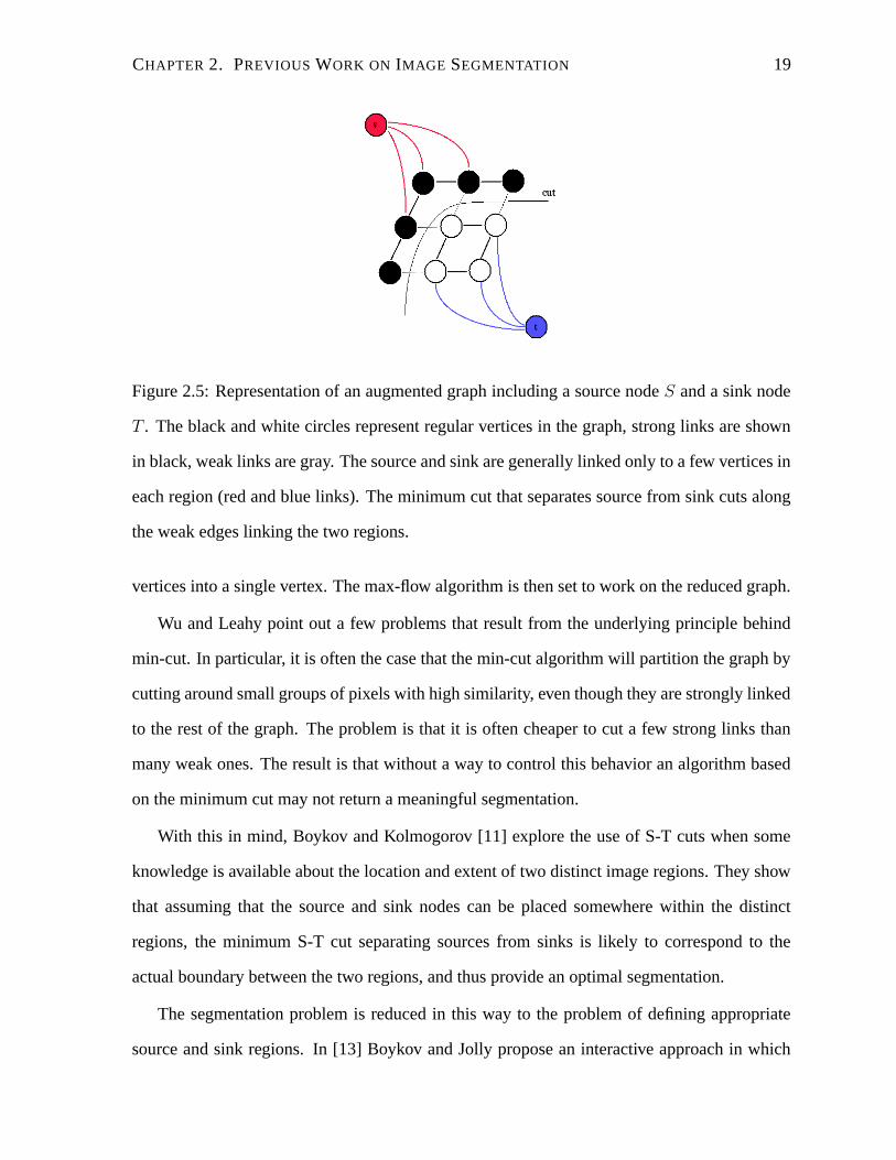
To calculate the minimum-cut efficiently, Wu and Leahy use a formulation of the problem

based on maximum-flows. Suppose that we are given a graph G′ that has been augmented

to contain two special nodes called source S, and sink T ; both source and sink nodes are

connected in some way to a subset of the original nodes from G with very large weights, as

illustrated in Figure 2.5.

Given this augmented graph, the problem is to find the smallest cut that completely discon-

nects source and sink nodes. Since the weights joining source and sink nodes to the original

nodes from G are large, the minimum cut separating sources and sinks will only contain links

from the original graph G. The computation of this S-T cut can be formulated as a maximum-

flow problem [32]. This formulation is based on viewing edges as pipes that carry water, where

the capacity of the edge to carry water is related to the edge’s strength and thus to the similarity

between the nodes spanned by the edge. If sufficient water is pumped through an edge, it will

become saturated. An increasing flow of water between two dissimilar regions A and B in

the graph will eventually saturate the subset of edges of least capacity that separate A from B.

The value of the flow that saturates these edges corresponds to the maximum-flow that can be

pumped between A and B, and the saturated edges make up the the minimum-cut separating

the two regions.

To approximate the optimal cut through the graph, Wu and Leahy take pairs of pixels in the

image, and compute the S-T minimum cut using one pixel as source, and the other as sink. To

approximate the minimum-cut through the graph, they choose the cut that yields the smallest

value among the S-T cuts corresponding to every possible pair of pixels within the image. They

use an algorithm due to Gomory and Hu [38] to carry out this process efficiently, but even so,

for large images the number of cuts that have to be evaluated becomes prohibitively large.

To address this problem, they also discuss a hierarchical version of the algorithm, intended

to work on large graphs where the standard method becomes impractical; the operating prin-

ciple of their improved approach is that links with strong weights are unlikely to be removed

as part of the min-cut. The size of the graph can be reduced by condensing strongly linked


Figure 2.5: Representation of an augmented graph including a source node S and a sink node

T . The black and white circles represent regular vertices in the graph, strong links are shown

in black, weak links are gray. The source and sink are generally linked only to a few vertices in

each region (red and blue links). The minimum cut that separates source from sink cuts along

the weak edges linking the two regions.

vertices into a single vertex. The max-flow algorithm is then set to work on the reduced graph.

Wu and Leahy point out a few problems that result from the underlying principle behind

min-cut. In particular, it is often the case that the min-cut algorithm will partition the graph by

cutting around small groups of pixels with high similarity, even though they are strongly linked

to the rest of the graph. The problem is that it is often cheaper to cut a few strong links than

many weak ones. The result is that without a way to control this behavior an algorithm based

on the minimum cut may not return a meaningful segmentation.

With this in mind, Boykov and Kolmogorov [11] explore the use of S-T cuts when some

knowledge is available about the location and extent of two distinct image regions. They show

that assuming that the source and sink nodes can be placed somewhere within the distinct

regions, the minimum S-T cut separating sources from sinks is likely to correspond to the

actual boundary between the two regions, and thus provide an optimal segmentation.

The segmentation problem is reduced in this way to the problem of defining appropriate

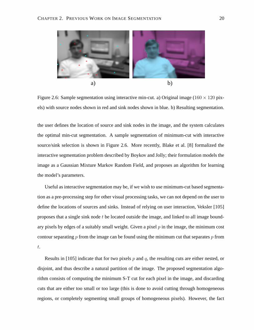
source and sink regions. In [13] Boykov and Jolly propose an interactive approach in which


a) b)

Figure 2.6: Sample segmentation using interactive min-cut. a) Original image (160 × 120 pix-

els) with source nodes shown in red and sink nodes shown in blue. b) Resulting segmentation.

the user defines the location of source and sink nodes in the image, and the system calculates

the optimal min-cut segmentation. A sample segmentation of minimum-cut with interactive

source/sink selection is shown in Figure 2.6. More recently, Blake et al. [8] formalized the

interactive segmentation problem described by Boykov and Jolly; their formulation models the

image as a Gaussian Mixture Markov Random Field, and proposes an algorithm for learning

the model’s parameters.

Useful as interactive segmentation may be, if we wish to use minimum-cut based segmenta-

tion as a pre-processing step for other visual processing tasks, we can not depend on the user to

define the locations of sources and sinks. Instead of relying on user interaction, Veksler [105]

proposes that a single sink node t be located outside the image, and linked to all image bound-

ary pixels by edges of a suitably small weight. Given a pixel p in the image, the minimum cost

contour separating p from the image can be found using the minimum cut that separates p from

t.

Results in [105] indicate that for two pixels p and q, the resulting cuts are either nested, or

disjoint, and thus describe a natural partition of the image. The proposed segmentation algo-

rithm consists of computing the minimum S-T cut for each pixel in the image, and discarding

cuts that are either too small or too large (this is done to avoid cutting through homogeneous

regions, or completely segmenting small groups of homogeneous pixels). However, the fact


that the cuts for two different pixels are either nested or disjoint leads to several ways to reduce

the size of the graph upon which the minimum cut must be computed; additional optimizations

are also discussed that reduce the number of pixels that need to be processed.

Finally, the algorithm is applied recursively to each previously extracted segment, thus

generating a segmentation hierarchy that goes from coarse to fine regions. Results shown in

the paper indicate that the algorithm is indeed capable of finding interesting image regions

without many of the associated artifacts that occur in typical min-cut segmentations. Is is

important to keep in mind that the images upon which the above algorithms work are usually

limited in size. This limitation is common to graph-theoretic algorithms, and is a consequence

of the amount of memory required to store the graphs associated with large images, and of the

computational cost of partitioning such graphs.

Boykov et al. [12] present an algorithm that relies on min-cut to perform energy mini-

mization efficiently. They address the problem of assigning labels to a set of pixels such that

the labeling is piecewise smooth, and consistent with observed data. They define a suitable

energy functional, and show that given an initial labeling, min-cut can be used to approxi-

mately minimize this functional with regard to two classes of operations that work respec-

tively on single labels, and label pairs. Other min-cut related algorithms can be found in [46],

and [108]. Ishikawa and Geiger [46] propose an interesting mixture between minimum cut

based grouping, and gray level thresholding. The algorithm locates image junctions, and then

uses a min-cut based algorithm to find the minimum set of gray level thresholds that will seg-

ment the image while preserving the junction structure. Their results show segmentations that

capture some of the structure in the image, however they also show some of the problems

inherent to gray level thresholding schemes, namely, splitting of homogeneous regions and

under-segmentation due to illumination effects, colour gradients, or texture.

In [108], Wang and Siskind propose a modification to the minimum cut criterion to reduce

the preference of minimum cut for small boundaries. They propose the use of minimum mean


cut, defined as

c(A,B) =cut(A,B)

L(2.10)

where L is the length of the boundary dividing A and B. Like other min-cut based algorithms,

the minimum mean cut is used recursively to produce finer segmentations. Wang and Siskind

present a polynomial-time algorithm for finding the minimum mean cut, and show results on

several images. It is interesting to point out that their algorithm uses an additional step of region

merging, since the minimum mean cut may lead to some spurious cuts where no image edge

exists. Wang [109] generalizes the minimum mean cut by using two edge weights to connect

pairs of vertices, the first weight comes from the similarity measure, and the second weight

corresponds to a normalization term based on the segmentation boundary length.

A different methodology is proposed by Gdalyahu, et. al, in [36]. They propose generating

a set of slightly different candidate segmentations for a given image, the candidate regions

are generated using an algorithm by Karger and Stein [53] which approximates the minimum

cut through a graph in a probabilistic fashion. The set of candidate segmentations provides

information about how often pairs of pixels are clustered together. This yields an estimate

of the probability that a given edge ei,j joining two pixels i and j is a crossing edge in an

’typical’ cut. The final segmentation is generated by removing all edges with greater than 50%

probability of being crossing edges. Shental et al. [96] describe a method that uses Generalized

Belief Propagation (GBP) to solve the typical cut problem, they show that the GBP formulation

is efficient, and develop a method for learning the affinity function that best describes similarity

from a labeled set of training images. Both of the above algorithms produce segmentations that

are qualitatively comparable to those offered by methods based on minimum cut.

Cho and Meer in [19] also use a set of slightly different segmentations to estimate the

probability of two pixels belonging to the same region. Their algorithm derives N different

versions of an initial segmentation by using the following procedure: A region adjacency graph

(RAG) which is initially set to represent the 8-connected neighborhood of pixels in the image is

reduced into several subgraphs using simple, local thresholds on gray level difference between


neighboring vertices. The edges corresponding to connections between homogeneous vertices

are removed. The resulting RAG contains nodes that represent homogeneous patches in the

image.

A probabilistic algorithm then merges pairs of neighboring nodes randomly, and the pro-

cedure is repeated with the new RAG until the RAG can not further reduced into subgraphs.

The above algorithm is repeated N times to generate N slightly different segmentations. Given

these different segmentations, the co-occurrence probability between pixel v and it’s ith neigh-

bor vi can be calculated with

p(v, vi) =Nv,vi

Ni = 0, . . . 7 (2.11)

where Nv,viis the number of times the pixels are assigned to the same region. The set of co-

occurrence probabilities for every pair of pixels defines the co-occurrence probability field of

the image. From this field, the consensus at each pixel v is calculated as

c(v) =255

8·

7∑

i=0

p(v, vi) (2.12)

the larger the value of c(v), the more likely it is that pixel v belongs to a homogeneous region.

The consensus at each pixel is used to produce a final segmentation using a modified version

of the RAG contraction procedure described above. The results presented in the paper are

qualitatively similar to those produced by the mean shift algorithm.

Tu et al. [103] propose a segmentation algorithm that uses Markov Chain Monte Carlo

simulation (MCMC) to determine the segmentation W that maximizes the Bayesian posterior

probability p(W |I)αp(I|W ) · p(W ). The prior probability p(W ) is calculated from known

statistics on the expected size of regions in an average image, as well as other conditions

imposed on W . A suitably defined Markov Chain, and Monte Carlo simulation, are then used

to estimate p(I|W ). Barbu and Zhu [2] also simulate Markov Chain dynamics to generate a

segmentation. They apply an algorithm from statistical mechanics known as the Swendsen-

Wang method to guide the Markov Chain process. Swendsen-Wang allows for a large number

of region labels to change at each step of the simulation; for this reason, it generally converges


much faster than regular MCMC algorithms which permit only one label change per simulation

step. Barbu and Zhu achieve a further increase in speed by starting the segmentation not with

individual pixels, but with small seed regions obtained from a simple pre-processing step.

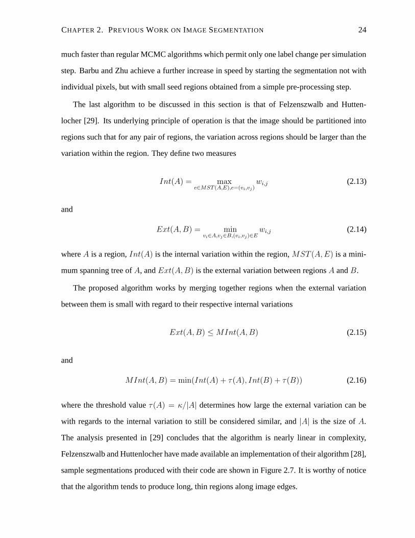
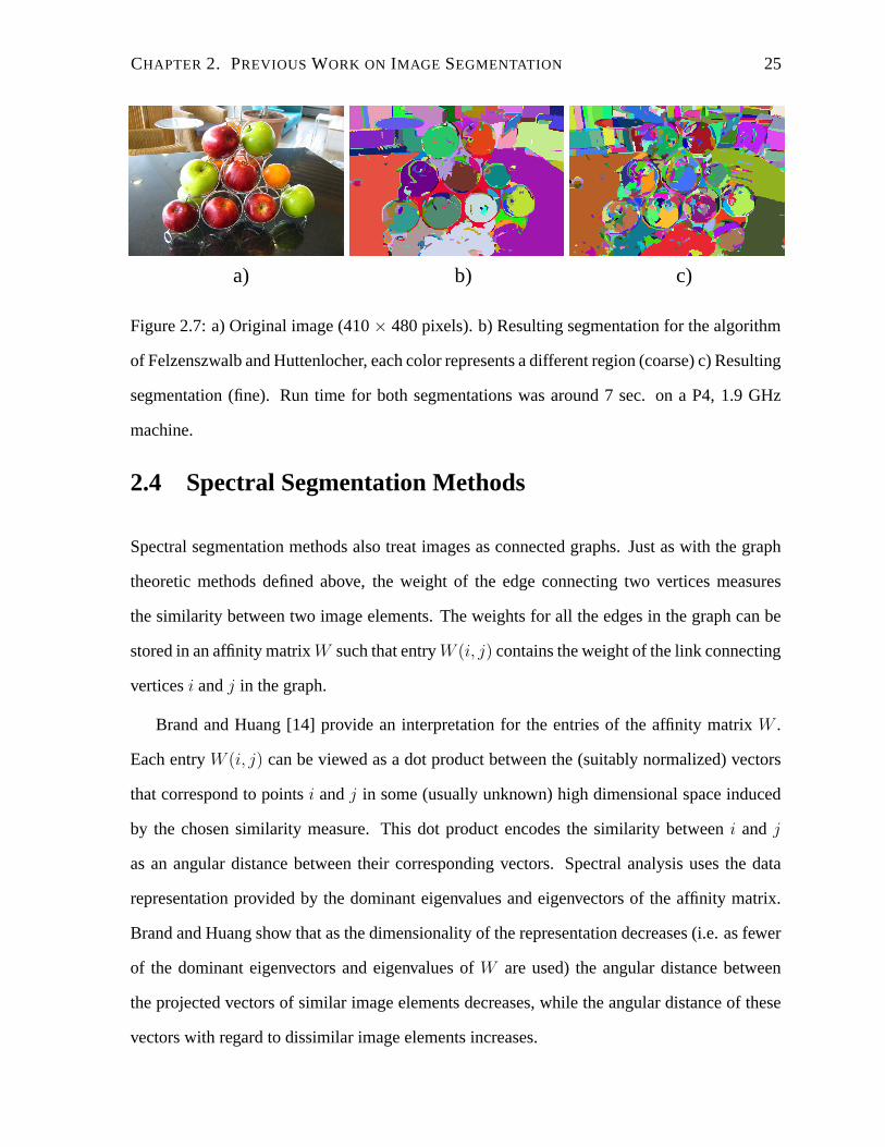
The last algorithm to be discussed in this section is that of Felzenszwalb and Hutten-

locher [29]. Its underlying principle of operation is that the image should be partitioned into

regions such that for any pair of regions, the variation across regions should be larger than the

variation within the region. They define two measures

Int(A) = maxe∈MST (A,E),e=(vi,vj)

wi,j (2.13)

and

Ext(A,B) = minvi∈A,vj∈B,(vi,vj)∈E

wi,j (2.14)

where A is a region, Int(A) is the internal variation within the region, MST (A,E) is a mini-

mum spanning tree of A, and Ext(A,B) is the external variation between regions A and B.

The proposed algorithm works by merging together regions when the external variation

between them is small with regard to their respective internal variations

Ext(A,B) ≤ MInt(A,B) (2.15)

and

MInt(A,B) = min(Int(A) + τ(A), Int(B) + τ(B)) (2.16)

where the threshold value τ(A) = κ/|A| determines how large the external variation can be

with regards to the internal variation to still be considered similar, and |A| is the size of A.

The analysis presented in [29] concludes that the algorithm is nearly linear in complexity,

Felzenszwalb and Huttenlocher have made available an implementation of their algorithm [28],

sample segmentations produced with their code are shown in Figure 2.7. It is worthy of notice

that the algorithm tends to produce long, thin regions along image edges.


a) b) c)

Figure 2.7: a) Original image (410 × 480 pixels). b) Resulting segmentation for the algorithm

of Felzenszwalb and Huttenlocher, each color represents a different region (coarse) c) Resulting

segmentation (fine). Run time for both segmentations was around 7 sec. on a P4, 1.9 GHz

machine.

2.4 Spectral Segmentation Methods

Spectral segmentation methods also treat images as connected graphs. Just as with the graph

theoretic methods defined above, the weight of the edge connecting two vertices measures

the similarity between two image elements. The weights for all the edges in the graph can be

stored in an affinity matrix W such that entry W (i, j) contains the weight of the link connecting

vertices i and j in the graph.

Brand and Huang [14] provide an interpretation for the entries of the affinity matrix W .

Each entry W (i, j) can be viewed as a dot product between the (suitably normalized) vectors

that correspond to points i and j in some (usually unknown) high dimensional space induced

by the chosen similarity measure. This dot product encodes the similarity between i and j

as an angular distance between their corresponding vectors. Spectral analysis uses the data

representation provided by the dominant eigenvalues and eigenvectors of the affinity matrix.

Brand and Huang show that as the dimensionality of the representation decreases (i.e. as fewer

of the dominant eigenvectors and eigenvalues of W are used) the angular distance between

the projected vectors of similar image elements decreases, while the angular distance of these

vectors with regard to dissimilar image elements increases.


If the original vectors are loosely clustered according to the chosen similarity measure,

the projection operation decreases the angular distance between elements of individual clusters

while increasing inter-cluster separation. This means that a clustering algorithm working on the

reduced-dimension representation of the data is more likely to be successful. Ng et al. [78] and

Brand and Huang [14] provide clustering algorithms based on such a reduced representation

of the original data. There are many different algorithms that use the spectral properties of the

affinity matrix, they differ in the number of eigenvectors/eigenvalues used, as well as in the

clustering procedure, but they rely on the principles described above. Weiss [111] discusses

the relationships between different spectral clustering methods.

Shi and Malik applied spectral analysis techniques to solve the image segmentation prob-

lem [97], [98]. Their formulation is related to the minimum cut algorithms described above.

Starting from the observation that minimum cut tends to prefer small boundaries, they define a

new cut measure between regions A and B as

Ncut(A,B) =cut(A,B)

assoc(A, V )+

cut(A,B)

assoc(B, V )(2.17)

where assoc(R, V ) =∑

i∈R,j∈V,(vi,vj)∈E wi,j is the total connection between elements in R and

all nodes in the graph. This Normalized Cut is not biased toward small regions, Shi and Malik

show that the cut that minimizes the Normalized Cut measure, also maximizes the association

between elements that belong to the same region.

Computing the Normalized Cut exactly for a given graph is an NP-complete problem, how-

ever, Shi and Malik show that an approximate solution can be obtained from the eigenvector

with the largest eigenvalue of the system

D−1/2WD−1/2x = (1 − λ)x (2.18)

where D is a diagonal matrix whose ith entry D(i, i) =∑

j w(i, j). Furthermore, they note that

succeeding eigenvectors provide sub-partitions to each of the groups from previous cuts. Their

segmentation algorithm consists of computing the affinity matrix, solving the above system for

the largest eigenvalue, and thresholding the corresponding eigenvector to obtain a partition of


the image. Several thresholds are tried, and the Normalized Cut is evaluated; the threshold

that yields the minimum Normalized Cut value is selected. This procedure is either applied

recursively to each of the detected regions, or eigenvectors with consecutively smaller eigen-

values are used to obtain the sub-partitions. Yu and Shi [117] study multi-way partitions in the

context of Normalized Cuts and Spectral Clustering. Meila and Shi [71] show a connection

between the eigenvectors and eigenvalues used in Normalized Cuts, and those of a Markov

matrix obtained by normalizing the affinity matrix W . They note that the Normalized Cuts

problem is strongly related to sets with low conductivity in the random walk described by the

Markov matrix.

The affinity measure proposed by Shi and Malik in [97] is the product of a spatial distance

term, and a brightness difference term. Belongie and Malik [5] study the integration of texture

similarity and brightness information into a single affinity measure, and Malik et al. [62], [63]

extend the above formulation so that the affinity measure incorporates several elements: A

brightness (or colour) affinity term, a texture similarity term, a boundary affinity term based on

intervening contours, and a spatial distance term that defines small neighborhoods over which

pixels are connected. A sample segmentation produced by Normalized Cuts using intensity

similarity and intervening contours is shown in Figure 2.8. This segmentation was produced

using the Normalized Cuts code available online at [23].

The boundary term depends on the probability that a contour exists between two pixels, and

is calculated from the responses of edge enhancing filters at various orientations. For texture,

they obtain a set of texture descriptors from filter responses across the image, and then use

these descriptors to measure similarity between small image neighborhoods. Their paper also

deals with the problem of assigning appropriate weights to each of the above components of

the affinity measure, based on the particular characteristics of an image patch.

The reader may have noticed that the image in Figure 2.8 is only medium size. This results

from one of the main shortcomings of spectral methods: The number of non-zero elements in

the affinity matrix is equal to the number of pixels in the image times the size in pixels of the


a) b) c)

e)d)

Figure 2.8: a) Original image (160 × 120 pixels). b) Resulting segmentation with 25 segments.

c) First eigenvector d) Second eigenvector. e) Third eigenvector.

neighborhood used in the affinity computation. For medium-sized images the computation of

the eigenvectors becomes computationally expensive, while for large images it may become

impossible to hold the affinity matrix in memory. The original Normalized Cuts formulation

relies on the fact that the affinity matrix can be made sparse, which allows the algorithm to

handle larger images than would be possible otherwise, and also allows for the use of optimized

eigensolvers that work on such sparse matrices. However, this is not sufficient for large images.

Fowlkes et al. [34], [33], and Belongie et al. [4] introduce a modification to the Normalized

Cuts framework that makes it possible to segment large images, or image sequences. The

modification is based on the Nystrom method for approximating the leading eigenvalues of a

matrix using only a small number of randomly sampled image pixels. These random samples

are used to build a smaller (non-square) affinity matrix whose leading eigenvectors can be

computed at a much lower computational expense than those of the affinity matrix for the full

image. These eigenvectors are then used to interpolate the complete solution to the Normalized


Cuts problem. Sharon et al. [94], [95] propose a different approach for making the Normalized

Cuts practical on large images. Their method solves a coarser Normalized Cut problem which

includes region based statistics in the affinity measure, and then interpolates the solution to

finer levels of detail, providing a hierarchy of segmentations for a given image.

2.5 Deformable Contours

Deformable contours were introduced as a technique for interactive image segmentation by

Kass et al., [54]. A deformable contour (also known as active contour, or snake) consists of

a parametric curve that is attracted to image features such as edges, lines, or corners. This

attraction is quantified by an energy function that has low values at places in the image that

contain the desired features. The energy function also incorporates a term that depends on

the shape of the curve, and can be used to bias the curve to take on smooth shapes (which is

something that previously discussed algorithms can not do, as they don’t model the shapes of

region boundaries explicitly), and a term that depends on user interaction, so that the curve can

be interactively pulled toward a desired location.

In [54], the energy function for a snake parameterized by v(s) = (x(s), y(s)) is defined as

Esnake =

∫ 1

0

Eint(v(s)) + Eimage(v(s)) + Econ(v(s))ds (2.19)

The internal energy Eint depends on the curvature of the snake, and controls how sharply the

curve can bend. The image energy Eimage depends on the type of feature toward which the

snake will be attracted. If, for example, Eimage is made to be inversely proportional to the

magnitude of the image gradient, the snake will be attracted to image edges. Finally, the term

Econ provides user specific control (see McInerny and Terzopoulos [69, 68]).

Given an initial curve, an iterative procedure based on gradient descent is used to drive the

snake toward a state of minimum energy. This energy minimization procedure is at the core of

all deformable contour formulations. Kass et al. show that given a reasonable initial guess for

the position of the snake, the active contour will converge to the desired image boundary. They


also note that if once the snake has converged, the boundary of interest moves a few pixels,

the energy minimization procedure will drive the active contour toward the new location of

the boundary. This behavior can be used to track slowly moving contours across an image

sequence.

There are two important issues that affect the results obtained with the active contour for-

mulation described above: First, the initial position of the curve will determine the final loca-

tion of the contour, since the energy function usually has many local minima, it is possible for

the snake to get stuck at one such minimum, and miss the globally optimal solution. Second,

segmenting multiple objects requires the initialization of multiple snakes, and adds another

layer of complexity to the energy minimization procedure, that now has to account for interac-

tions between different contours.

To solve the initialization problem, as well as to achieve a certain measure of automation,

it is common to initialize a set of ’seed’ contours all over the image. The contours are initially

small, but are biased to grow by the addition of a ’balloon’ force to the energy functional. The

state of minimum energy is achieved when the balloon force and the other terms in the energy

functional balance each other. The reader is referred to [15], [51], [99], and [118] among

others for extensions and modifications to the original active contours. In a related approach,

Jermyn and Ishikawa [49] propose an energy minimization scheme that incorporates boundary

and region properties. Their energy functional is normalized by contour length to avoid a bias

toward larger contours. More recently, Paragios [82] proposes an alternate formulation for

active contours which uses level set methods to control the evolution of the curve, Paragios

and Deriche [83] describe the use of these contours for image segmentation, and Kadir and

Brady [52] proposes a Level Set method incorporating region competition.

With such enhancements, active contour formulations have proven successful for the seg-

mentation of images in which regions are relatively homogeneous, and with simple back-

grounds. However, images that are rich in edge energy become problematic, the energy func-

tion develops a large number of local minima, and gradient descent methods used to evolve the


contour become attached to sub-optimal solutions. The issue of contour initialization also be-

comes more problematic, and in many instances, can prevent the contours from finding salient

boundaries.

2.6 Image Statistics and Learning for Segmentation

At the beginning of this chapter we mentioned that there is an ongoing effort to use the statis-

tics of natural images to help in the design and evaluation of image segmentation algorithms.

Martin, et. al, [66] present results of segmentations produced by several human observers on a

sizable number of images; their findings indicate that segmentations created by human subjects

have a significant amount of consistency

Figure 2.9 shows three images from their image database, along with several segmentations

produced by human observers. It is clear that different subjects segment the scene at different

levels of detail, but the important characteristic of all the segmentations is that regions proposed

by a human at a finer level of detail will merge in such a way that they yield the larger regions

proposed by a different observer at a coarser level.

With the above considerations in mind, Martin et al. propose two of error measures that can

be used to evaluate segmentation results from a segmentation algorithm. These error measures

are based on counting the number of pixels that are assigned to different regions in two different

segmentations of the same image, and are tolerant to variations due to the level of detail in the

corresponding segmentations. The local refinement error is defined as

E(S1, S2, pi) =|R(S1, pi)\R(S2, pi)|

|R(S1, pi)|(2.20)

where R(S, pi) is the set of pixels assigned to a region S in the segmentation which contains

pixel pi, \ represents the set difference operation, and | · | is the set cardinality.

The above error measure evaluates to 0 whenever two regions are identical, or when re-

gion S1 is a subset of region S2 (which gives this measure its robustness to variation due to


Figure 2.9: Three sample images from the Berkeley Segmentation Database, and correspond-

ing segmentations from different human observers.


different levels of detail in the segmentations). It is not symmetric, so the ordering of regions

is important. Using the above error measure, two error metrics for the complete image are

proposed

GCE(S1, S2) =1

nmin(

∑

i

E(S1, S2, pi),∑

i

E(S2, S1, pi)) (2.21)

and

LCE(S1, S2) =1

n

∑

i

min(E(S1, S2, pi), E(S2, S1, pi)), (2.22)

where n is the number of pixels in the image. The GCE, or Global Consistency Error only

considers refinements in one direction (i.e. every region in one of the segmentations must be

identical to, or a refinement of a region in the other segmentation). LCE, or Local Consistency

Error allows for refinements in either direction.

The results presented in [66] show that when two segmentations of the same image pro-

duced by different human observers are compared, the resulting errors are small across the

entire set of test images, this lends weight to the claim that segmentations produced by hu-

man observers are consistent. The error measures presented above provide a framework for

the evaluation of segmentation algorithms against a set of images for which ’ground truth’ is

available. Martin et al. compare the segmentations produced by the Normalized Cuts algorithm

with human segmentations, and conclude that the algorithm performs consistently worse than

human observers, but better than a random segmentation.

As a final note, Martin et al. evaluate the probability that two pixels are assigned to the

same region for a particular image cue. Their results show that as expected, proximity and

similarity are good indicators of whether pixels belong in the same region, and that regions in

the segmentation tend to be convex. They also find that the areas of regions in natural images

are distributed according to a simple power law.

The existence of a database of human segmentations from which some statistics of natural

images can be computed makes it possible to design segmentation algorithms based on such

statistics. Martin et al. [67] propose an edge extraction algorithm trained using the human

segmentations, they compare their edge extraction algorithm against Canny’s edge detector,


and against the human segmentations, and find that their edge detector has better performance

(though still significantly worse than human).

Ren and Malik [87] evaluate several region similarity measures that incorporate proximity,

intensity, texture similarity, and boundary smoothness. They train a classifier to combine these

cues so as to obtain the best possible performance on their training data, and show segmen-

tation results for their method. Fowlkes et al. [35] also evaluate the performance of different

grouping cues, and propose ways to train classifiers that combine these cues in a appropriate

manner. Finally, Heiler and Schnorr [43] use image statistics along with deformable contours

for segmentation.

2.7 Open Issues and State of the Field

The preceding sections provide an overview of the field of image segmentation, the review

shows that many current algorithms are able to produce reasonable results on images of mod-

erate complexity, several of these algorithms are efficient enough that they can be used as a

pre-processing stage for higher level vision tasks such as recognition and tracking. The exist-

ing research has indeed gone a long way toward achieving robust, high quality segmentations

without a-priori knowledge about particular images or image classes.

However, there are still several challenges facing current segmentation algorithms. Compu-

tational efficiency is still a concern when the processing of large affinity matrices is part of the

segmentation process, ultimately, a segmentation procedure can become impractically slow, or

require extremely large amounts of memory. This has limited the size of the images that can

be processed using many recent algorithms. However, we expect that the constant increase in

computational power and storage capacity of modern computers should progressively reduce

this limitation.

The definition of a good similarity measure for general images remains an open issue. There

is a general consensus in the literature that a robust image segmentation algorithm should com-


bine multiple image cues and estimate similarity based on this combination, but so far there

are few algorithms that use more than a single cue as a similarity measure, and only recently

has a significant effort been dedicated to designing similarity measures based on the statistics

of natural images, and human-generated segmentations. The design of a good similarity mea-

sure is tied to the robustness of the segmentation algorithm in dealing with surface markings,

lighting artifacts, and image texture.

Evaluating the output of segmentation algorithms is still problematic. The work of Martin

et al. [66] presents a significant advance in this direction by providing segmentation results that

can be used as a baseline for comparing the output of different segmentation methods, as well

as suitable error metrics to quantify the performance of the algorithms in terms of the quality

of their segmentations. However, at this time, to our knowledge only the Normalized Cuts

algorithm has been evaluated in this way, and the results of this evaluation can’t be interpreted

in a meaningful way in the absence of comparative results for other segmentation methods.

Finally, the general question of how far it is possible to go with purely bottom-up ap-

proaches remains unanswered. The gap observed by Martin et al. [66] between the performance

of the Normalized Cuts algorithm and human perception could very well be due to the use by

human observers of higher-level knowledge. Examples such as those shown in Fig 2.1 suggest

that at some point higher-level vision will be required to disambiguate and refine the results

of bottom-up image processing, but the development of segmentation methods that integrate

bottom-up and top-down analysis has yet to be explored in any degree of detail.

In the following chapter, a new bottom-up segmentation algorithm will be introduced. The

algorithm is based on S-T minimum cut for finding boundaries between regions. We will de-

scribe the use of spectral embedding to generate candidate source and sink regions, discuss the

properties that such candidate regions must have so that the segmentation will be meaningful,

and at the same time, show a connection between spectral embedding and anisotropic image

smoothing.

Date post:	23-May-2020
Category:	Documents
Upload:	others
View:	26 times
Download:	0 times

Chapter 2 Previous Work on Image Segmentationstrider/publications/Chapter2.pdf · Chapter 2...

Documents