Chapter 2 T ranscritical refrigerating devices · tion of greenhouse gases in the Earth’s...

Chapte r 2

T ranscritical re frig e rating de v ice s

2 .1 Reaso ns o f inte re st

Co nv entio na l mo deling a ppro a ches rema in co nfined in the cha ra cteristic dimen-

sio na l sca le o f the fina l user, while the fo rmula tio n o f lower-sca le mo dels a ims to

co mplete the picture o f the pheno meno n by co nsidering a s ma ny sca les a s po ssible in

o rder to increa se the a ccura cy a nd the suita bility o f the descriptio n. The result ca n

be v ery fa r fro m the immedia te sensitiv ity o f the fina l user beca use it is usua lly much

mo re co mplica ted, but this do es no t mea n tha t this descriptio n is less useful fo r the

fina l desig n purpo ses. A simpler mo del ca n a ppea r nicer but it will be less powerful

in predicting so mething rea lly new, which wa s no t implicitly included in the a v era g ed

q ua ntities co nsidered a s input da ta .

In the fo llowing , a pa rticula r techno lo g ica l a pplica tio n, i.e. the tra nscritica l re-

frig era ting pla nts with ca rbo n dio x ide a s wo rk ing fluid, will be co nsidered. This

a pplica tio n ha s been selected fo r the fo llowing rea so ns.

� First o f a ll, the po ssibility o f using a g a in the ca rbo n dio x ide a s wo rk ing fluid in

the refrig era ting pla nts with perfo rma nce which tries to a ppro a ch tha t o f usua l

dev ices ba sed o n sy nthetic fluids is chiefly due to a minia turiza tio n pro cess.

In pa rticula r, this minia turiza tio n pro cess dea ls with the desig n o f mini/ micro

cha nnel co mpa ct hea t ex cha ng ers a nd it ca n be co nsidered a g eo metrica l im-

2 9

30 CHAPTER 2 . TR ANSCR ITICAL R EFR IG ER ATING D EVICES

provement, since no additional functional elements are added to these devices.

� Secondly, at this development stage, some uncertainties exist about the heat

transfer properties of carbon dioxide and this will allow us to appreciate the

effects of the lower scales. In fact, the peculiar phenomena, which rise close

to the critical point, make it very difficult to obtain an accurate experimental

measurement of the heat transfer parameters (end-user scale). This situation

partially justifies the great discrepancies that exist among different phenomeno-

logical correlations, which have been proposed throughout the last years. In this

case, to formulate a lower-scale model means to go back to more fundamental

phenomena (underlying scale), which affect the heat transfer parameters, trying

to obtain some additional information by directly modeling them.

� Finally, the permeation of carbon dioxide throughout the gaskets of the connect-

ing components is a critical issue because of the high operating pressures; this

undesired phenomenon allows us to appreciate the practical effects of modeling

fluid flow in micro-structures.

This chapter is organized as follows. Some information about the history of car-

bon dioxide as refrigerant, its thermodynamic and thermo-physical properties and

the specific issues of the consequent transcritical cycles are reported. The design of

the experimental test rig and the results of the experimental plan are discussed. Fi-

nally, a reduced model fitting the previous experimental data is developed and some

interpolating results are reported.

2.1.1 Trends of regulation on refrigeration technology

O ver the last decades, the refrigeration, air conditioning and heat pump industry

has been forced through major changes caused by restrictions on refrigerants. For

2.1 . REASO NS O F INTEREST 31

this reason, research and development in this field have been strongly influenced by

environmental issues. These constraints are becoming more and more restrictive with

respect to the utilization of synthetic fluids in the refrigeration technology. For this

reason, some synthetic fluids that were once expected to be acceptable permanent

replacement fluids are now on the list of regulated substances due to their impact on

the environment. The present refrigeration technology, and even more the future one,

will not be allowed to develop devices without taking care of the effects on the global

environment.

Essentially the great majority of the synthetic fluids which have been developed

for the refrigeration technology derive from paraffinic hydrocarbons and they can be

obtained by substituting the hydrogen atoms with atoms of other substances, like

chlorine and fluorine. D epending on the final result of this process, the synthetic

fluids can be subdivided in three categories:

� the chlorofluorocarbons (CFCs), which are the compounds made from carbon,

chlorine and fluorine;

� the hydrochlorofluorocarbons (H CFCs), which are the compounds made from

carbon, hydrogen, fluorine and chlorine;

� the hydrofluorocarbons (H FCs), which are the compounds made from carbon,

hydrogen and fluorine.

Some widespread synthetic fluids and some natural fluids used in the refrigeration

technology are reported in Tab. 2.1.

All the regulations for refrigeration technology refer to some indexes, which allow

us to quantify the effects of the synthetic substances on the global environment. The

two most serious effects of the human activity on the global environment concern

32 CHAPTER 2. TRANSCRITICAL REFRIGERATING DEVICES

Table 2.1: Some widespread synthetic fluids and some natural fluids in refrigerationtechnology (ASHR AE codes are adopted).

Chlorofluorocarbons (CFCs)ASHR AE Code Chemical Formula Chemical Name

R-11 C Cl3 F TrichlorofluoromethaneR-113 C Cl2 F C ClF2 TrichlorotrifluoroethaneR-114 C ClF2 C ClF2 DichlorotetrafluoroethaneR-12 C Cl2 F2 DichlorodifluoromethaneR-13 C ClF3 ChlorotrifluoromethaneR-14 C F4 Tetrafluoromethane

R-C318 C4 F8 Octafluorocyclebutane

Hydrochlorofluorocarbons (HCFCs)R-123 C H Cl2 C F3 DichlorotrifluoroethaneR-21 C H Cl2 F DichlorofluoromethaneR-22 C H ClF2 Chlorodifluoromethane

Hydrofluorocarbons (HFCs)R-134 a C H2 F C F3 1,1,1,2-tetrafluoroethaneR-15 2 C H3 C H F2 1,1-difluoroethaneR-23 C H F3 Trifluoromethane

MixturesR-4 01A R-22/15 2a/124 (5 3/13/34 ) Ternary mixtureR-4 07C R-32/125 /134 a (23/25 /5 2) Ternary mixtureR-4 10A R-32/125 (5 0/5 0) B inary mixtureR-5 07 R-125 /14 3a (5 0/5 0) B inary mixture

Natural FluidsR-115 0 C H2 = C H2 Ethene (ethylene)R-127 0 C H3 C H = C H2 Propene (propylene)R-17 0 C H3 C H3 EthaneR-290 C H3 C H2 C H3 PropaneR-5 0 C H4 MethaneR-6 00 C H3 C H2 C H2 C H3 B utaneR-6 00a C H (C H3)3 2-methyl propane (isobutane)R-7 17 N H3 AmmoniaR-7 18 H2 O W aterR-7 28 N2 NitrogenR-7 29 N2/O2/A (7 6 /23/1) AirR-7 32 O2 OxygenR-7 4 0 A ArgonR-7 4 4 C O2 Carbon dioxide

2.1. REASONS OF INTEREST 33

the anthropic (or enhanced) global warming due to the greenhouse effect and the

depletion of the stratospheric ozone layer.

The greenhouse effect is a naturally occurring process that aids in heating the

Earth’s surface and atmosphere. It results from the fact that certain atmospheric

gases, such as carbon dioxide, water vapor, and methane, are able to change the en-

ergy balance of the Earth by being able to absorb relatively long-wave radiation from

the Earth’s surface. These gases are called greenhouse gases. Without the greenhouse

effect, life on this planet would probably not exist as the average temperature of the

Earth would be too low. The relevance of this effect is controlled by the concentra-

tion of greenhouse gases in the Earth’s atmosphere. All of the major greenhouse gases

have increased in concentration since the beginning of the industrial revolution. Some

evidences exist which seem to suggest that a result of these higher concentrations is

an enhanced global warming which could affect the planet climate. The most com-

mon greenhouse gases include: carbon dioxide (CO2); methane (CH4); nitrous oxide

(N2O); the synthetic fluids involved in the refrigeration technology (CFCs, HCFCs

and HFCs); and tropospheric ozone (03). Even though the synthetic fluids involved

in the refrigeration technology are the strongest greenhouse gases per molecule, they

account for the 25% of the change in the intensity of the Earth’s greenhouse effect,

i.e. less than the contribution due to the carbon dioxide which accounts for the 50%.

In order to estimate the effects of a chemical substance with regard to the anthropic

global warning, the global warming potential (G W P ) may be considered. This index

relates the potential of a greenhouse gas to that of carbon dioxide over a 100-year

period and it is determinated by the Intergovernmental Panel on Climate Change.

The synthetic fluids created for the refrigeration technology are characterized by

G W P s which are three orders of magnitude higher than the G W P of carbon dioxide,


which has GWP = 1 by definition. Another very popular index is the total equivalent

warming impact, T E WI, used to measure the overall contribution of a technology to

global warming. This index is slightly less rigorous than the previous one because it

depends as well on the considered technology which uses the fluid and the installation

location of the device but it still gives good relative comparisons. The T E WI index

takes into account the whole life cycle of the considered device and the indirect effects

on the global environment in order to allow proper device operation. This is important

for comparison involving synthetic fluids and natural fluids, because the natural fluids

usually imply lower efficiency since they are not designed for any specific application.

Since the synthetic fluids involved in refrigeration have some effects on the enhanced

global warming, they are included in the K yoto Protocol. The K yoto Protocol has

been defined by the United Nations Framework Convention on Climate Change during

the world conference at K yoto (Japan) in 1997, in order to reduce the anthropogenic

carbon dioxide equivalent emissions of greenhouse gases. The K yoto Protocol is not

yet in force since the number of countries that have ratified it is not sufficient, but

the general trends which inspire this protocol are widely shared and they will affect

the technological development whether it will be ratified or not.

While the synthetic fluids for refrigeration are not the leading causes of the en-

hanced global warming, the situation is completely different if the depletion of the

stratospheric ozone layer is considered. The ozone layer is a region of concentra-

tion of the O3 molecule in the Earth’s atmosphere. The layer sits at an altitude of

about 10-50 km, with a maximum concentration in the stratosphere at an altitude

of 25 km. In recent years, some evidences exist that the stratospheric ozone layer is

becoming thinner, primarily at the poles, and this phenomenon is being called the

ozone hole. The ozone layer naturally shields Earth’s life from the harmful effects


of the solar ultraviolet radiation. A severe decrease in the concentration of ozone

in the ozone layer could lead to harmful effects, like an increase in the number of

cases of skin cancer, a sharp increase in cataracts and sun burning, suppression of

immune systems and a reduction in the growth of ocean phytoplankton. The ozone

layer is naturally produced by the solar ultraviolet radiation which hits the strato-

sphere. The CFCs, and secondly the HCFCs, created at the Earth’s surface slowly

drift upward to the stratosphere where ultraviolet radiation from the sun causes their

decomposition and the release of chlorine. Chlorine in turn attacks the molecules of

ozone converting them into oxygen molecules. The human activities are altering the

amount of stratospheric ozone, with the main culprits being human-made CFCs and

HCFCs.

The ozone depletion potential (OD P ) is a measure of the ability of a compound

to reduce the amount of stratospheric ozone and it can be used to quantify the effects

of a chemical substance on the global environment. The OD P is the technical tool

adopted by the Montreal Protocol and it is defined as the ratio of calculated ozone

column change for each mass unit of a gas emitted into the atmosphere relative to

the calculated depletion for a reference gas (R-11). The Montreal Protocol is the first

worldwide agreement designed to protect human health and the environment against

the adverse effects of the depletion of the stratospheric ozone layer. The protocol

is administered by the United Nations Environment Program, which maintains the

list of ozone-depleting substances that are targeted for control practices, reductions,

or total phase-outs. The OD P formed the primary basis for inclusion on the list,

although the final list was a product of international negotiation. The Montreal

Protocol divides ozone depleting substances into a variety of lists of chemicals that are

subject to different control requirements. Countries that signed the treaty committed


to:

1. reduce consumption or production of HCFCs to 1989 levels;

2. stop consumption or production of chemicals on G roup 2 after January 1st, 1994

(Halo n 1211, Halo n 1301, and Halo n 2402);

3. stop consumption or production of chemicals on G roup 1 after January 1st, 1996

(R-11, R-12, R-113, R-114, and R-115);

4. stop consumption or production of chemicals on G roups 1, 2 and 3 after January

1st, 1996 (R-13, R-111, R-112, R-211, R-212, R-213, R-214, R-215, R-216, R-

217, carbon tetrachloride, and 1,1,1-trichloroethane);

5. reduce consumption or production of methyl bromide to 75% of 1991 levels

beginning in 1999.

The Montreal Protocol mandated an end to the production and consumption of the

major CFCs, halons, hydrobromofluorocarbons (HB FCs) and methyl bromide by

1996, while the HCFCs are tolerated but they are not considered acceptable per-

manent replacement fluids. Implementation of the Montreal Protocol was dependent

on national regulation. In particular, the European Union (EU) regulation on ozone

depleting substances, EU 2037/2000 applies from October 1st 2000, upon which date

the previous regulation, EU 3093/94, was repealed. The remarkable feature of this

EU regulation is that in some cases it goes beyond the requirements of the Montreal

Protocol, particularly with regard to the HCFCs. The key points are discussed in

the following.

� New bans on the supply and use of CFCs, Halo n s , 1,1,1-trichloroethane, car-

bon tetrachloride, HB FCs and bromochloromethane. These bans apply from

October 1st 2000 for most applications, although certain delays and exceptions

apply. The bans on these substances apply to both virgin and recycled material.


� Significant revisions to the control on use of HCFCs. This adds a number

of new controls to those specified in the previous EU regulation. HCFCs

will not be allowed to be used in new equipment from January 1st 2001 (with

some exemptions) and servicing HCFC systems will be restricted to the use of

recovered/reclaimed refrigerant from January 1st 2010 to December 31st 2014.

All the major end use sectors for HCFCs are subject to new use controls.

� Tougher requirements regarding the recovery of ozone depleting substances from

products and equipment and to prevent leakage from systems.

� A ban on the supply of ozone depleting substances in disposable containers

(except for essential uses).

� A revised timetable for the supply of HCFCs. The timetable was designed to

match the new HCFC end use controls. Some cuts came into effect in 2001 and

there was a substantial cut by 2003. No virgin HCFCs can be supplied after

the end of 2009.

� A ban on the import of products containing ozone depleting substances. This is

immediate for all ozone depleting substances except HCFCs, which are char-

acterized by specific use control dates.

� A ban on the export of virgin and recycled CFCs and Halons and products

containing them, although certain exemptions apply.

� A new timetable for the phase out of EU production of HCFCs.

A complete discussion about the regulation on this subject is beyond the purposes

of the present work. It is important to point out that, in the international regulation,

an unquestionable trend exists, which aims to reduce and eventually eliminate the


utilization of synthetic fluids in refrigeration technology. The consecutive regulations

on this subject become more and more restrictive and they implicitly suggest to move

to natural fluids in order to find different long-term solutions. Instead of continuing

the search for new chemicals, there is an increasing interest in technology based on

ecologically safe refrigerants, i.e. fluids like water, air, noble gases, hydrocarbons,

ammonia and carbon dioxide [20].

2.1.2 Recovery of natural fluids

The ASHRAE (American Society of Heating, Refrigerating and Air-Conditioning

Engineers) has set more than two thousand fluids theoretically suitable as working

fluids for vapor compression. Just a few of the proposed ones are natural, i.e. are

naturally present in the Earth biosphere. As outlined in the previous section, envi-

ronmental problems have gained increasing importance and they suggest a recovery

of natural fluids. The possible natural fluids which could be used in refrigeration

based on vapor compression are:

� ammonia (R-717);

� hydrocarbons (mainly isobutane R-600a and propane R-290);

� carbon dioxide (R-744);

� air (R-729);

� argon (R-740).

The most important characteristics of these fluids are reported in Tab. 2.2. The

usual operating temperatures for vapor cycles in air conditioning systems are included

between 0�

and + 50�

. In this range of temperature, air and argon are present

only as in the gas state, as it is easy to verify by considering the critical point, and

for this reason those fluids have not been included in Tab. 2.2. It must be pointed out


Tab

le2.

2:C

ompar

ison

amon

gso

me

synth

etic

and

nat

ura

lre

frig

eran

ts(s

ourc

e[2

0]).

R-1

2R

-22

R-1

34a

R-4

07C

R-4

10A

R-7

17R

-600

aR

-290

R-7

44O

PD

/GW

Pa

1/85

000.

05/1

700

0/13

000/

1600

0/19

000/

00/

200/

30/

1Fla

mm

ability

/Tox

icity

N/N

N/N

N/N

N/N

N/N

Y/Y

Y/N

Y/N

N/N

Mol

ecula

rm

ass

[kg/k

mol

]12

0.9

86.5

102.

086

.272

.617

.058

.144

.144

.0N

orm

alboi

ling

poi

ntb

[

� ]−

29.8

−40

.8−

26.2

−43

.8−

52.6

−33

.3−

11.6

−42

.1−

78.4

Cri

tica

lpre

ssure

[MP

a]

4.11

4.97

4.07

4.64

4.79

11.4

23.

644.

257.

48C

riti

calte

mper

ature

[

� ]11

2.0

96.0

101.

186

.170

.213

3.0

134.

796

.731

.1R

educe

dpre

ssure

c[−

]0.

070.

100.

070.

110.

160.

040.

040.

110.

47R

educe

dte

mper

ature

d[−

]0.

710.

740.

730.

760.

790.

670.

670.

740.

90R

efri

gera

tion

capac

ity

e[k

J/m

3]

2734

4356

2868

4029

6763

4382

1509

3907

2254

5Fir

stco

mm

erci

aluse

asre

frig

eran

t19

3119

3619

9019

9819

9818

59?

?18

69

aG

lobalw

arm

ing

pot

enti

alin

rela

tion

to10

0ye

ars

inte

grat

ion

tim

e,fr

omth

eIn

terg

over

nm

enta

lPan

elon

Clim

ate

Chan

ge(I

PC

C).

bA

SH

RA

Ehandbook

2001

fundam

enta

ls.

cR

ati

oof

satu

rati

onpre

ssure

at27

3.1

5K

tocr

itic

alpre

ssure

.dR

ati

oof

273

.15

Kto

crit

icalte

mper

atu

re.

eV

olu

met

ric

refr

iger

ation

capaci

tyat

273.1

5K

.


that carbon dioxide, due to its critical temperature 31.1 � , realizes a transcritical

cycle for the considered operating conditions, that is a refrigerating cycle that works

between two different pressures: evaporating pressure below the critical one and the

heat rejection pressure above. All the other fluids are characterized by the usual

configuration and phase-change processes exist for both operating pressures.

A complete review of all refrigeration systems where natural fluids can be suitabil-

ity adopted and a serious comparison among possible natural candidates according

to the considered application is beyond the purposes of the present work. Some good

reviews about this subject may be considered [22, 23]. In order to compare the suit-

ability of the considered natural fluids for air conditioning applications, only some

essential features will be discussed [21].

1. Working pressure

The operating pressures for R-717 and R-290 are very similar, while the R-600a

is characterized by lower values and R-744 is characterized by much greater

pressures. Increasing the operating pressure of the working fluid is usually con-

sidered a difficulty and for this reason the previous comparison seems to be

unfavorable to carbon dioxide. However it must be pointed out that high work-

ing pressure fluids are less penalized than lower pressure fluids when taking into

account temperature drops related to pressure drops, being the same the cross-

ing velocity. For this reason, we can increase the crossing velocity inside heat

exchangers obtaining higher heat transfer coefficients, and so a better efficiency

in the heat transfer process.

The worry about carbon dioxide high working pressures is not justified if we

consider that its volumetric latent heat is higher than that of all other natural

fluids. A large value of volumetric latent heat implies a reduction of the volume


flow rate to be run to obtain the same refrigeration capacity. High operating

pressure and the related high vapor density make it possible to employ small

size piping and heat exchangers with small internal volume. For this reason the

danger linked to a possible explosion is small because this danger is related to

the mechanical energy inside the circuit, which is proportional to volume. For

the same reason, carbon dioxide implies a reduction of the refrigerant charge

and consequently more compact compressors and lighter machines. The last

feature is particularly relevant for airborne systems, as will be discussed later

on.

Even though the carbon dioxide high working pressures do not imply a real

explosion danger, they may induce some leakage problems. Since carbon diox-

ide is a natural fluid, possible leakages do not affect the environment but they

usually hinder the thermodynamic performance of the systems. This problem

may be reduced by considering special stainless steel connections. However

cost reduction suggests to consider connecting components made of elastomers.

Unfortunately the thermodynamic properties of carbon dioxide cause a high

solubility as well as a moderate diffusion velocity in elastomers. For this rea-

son, compared to other natural gases, the permeation rate results significantly

higher. Special care must be taken in order to ensure acceptable performances

during operating conditions. This feature will be further discussed at the end

of Chapter 5.

2. Heat transfer performance

Considering the attitude to exchange heat, the worst among the selected natural

fluids previously considered is isobutane (R-600a). This can be seen from the

low thermal conductivity of the liquid and mainly the values of the vapor den-


sity and pressure. Propane and ammonia behave better. Indeed, carbon dioxide

shows the best heat transfer performance. In the usual operative conditions for

the working fluid in refrigerating machines and heat pumps, the thermophysical

properties of carbon dioxide are favorable to produce high heat transfer coef-

ficients in the heat exchangers of the equipment (of suitable geometry), often

higher than those commonly obtained with traditional synthetic refrigerants.

3. Compatibility with other materials

Ammonia is the worst natural fluid with regard to corrosion problems. In

fact, the refrigerating plants based on ammonia as working fluid should involve

steel or aluminum components, instead of copper in order to avoid corrosion

problems. For the same reason, only few hermetic compressors exist for this

fluid. Ammonia is virtually insoluble in the most commonly used lubricating

oils.

On the other hand, hydrocarbons and carbon dioxide do not display drawbacks

in this respect and are compatible with common materials and oils. In par-

ticular, carbon dioxide is an inert product and is compatible with all common

materials encountered in a refrigeration circuit, both metals and plastics or

elastomers.

4. Safety

Ammonia is toxic and the effects due to direct exposure can vary from eyes

irritation up to death according to considered concentrations. Moreover, am-

monia is flammable in air and this induces to avoid any possibility of direct

contact between the circuit containing ammonia and the air to be distributed

into conditioned space.


Hydrocarbons are not toxic, but they are flammable and for this reason they

need safety constraints too. Some evidences exist that, in systems based on

hydrocarbons, small refrigerant leakage in a confined space can easily provoke

fire or explosions. Many markets in the world are quite restrictive to application

of hydrocarbons in vapor compression systems. Even though the car air condi-

tioning devices using hydrocarbons are allowed in Australia, the regulation on

this subject is very severe.

Finally, carbon dioxide is a product that displays no special local safety problem,

as it is non-flammable and non-toxic. However it is a gas heavier than air, it can

accumulate in the lower part of a non-ventilated ambient, causing suffocation

for lack of oxygen.

The introduction of natural refrigerants requires the development of improved

technology in processes and components suitably adapted to their positive and nega-

tive characteristics, and the formulation of safety codes of practice and standards for

systems and component design, installation and operation [24]. In particular, for am-

monia and hydrocarbon applications there is a great need for uniform international

regulations and standards based on accepted quantitative risk assessment studies.

However, the possible widespread diffusion of ammonia and hydrocarbons seems a

distant possibility in Europe and in U.S.A., with the exception of few applications

which include supermarkets and domestic refrigerators respectively. Even though re-

search on alternative refrigerants is continuing on many parallel paths, carbon dioxide

is a very promising working fluid for vapor compression refrigerating systems.

Recent researches on transcritical carbon dioxide systems have investigated a va-

riety of possible applications, which can make suitable use of the thermo-physical

(thermodynamic and transport) properties of this natural fluid. For several reasons,


mobile air conditioning applications were among the first to be considered [20]. In

particular, the automotive air conditioning sector yields many research programs,

mostly with funding from involved industries [25– 27]. In automobiles, a natural fluid

for refrigerating systems would allow us to avoid any future regulation constraints

due to the high leakage rates which characterize this application. Moreover, the high

temperature of heat rejection allows us to design ultra-compact gas coolers, which

increase energy efficiency and reduce the packaging problems due to integration with

other subsystems in closed spaces (under-hood space management). Finally, the car-

bon dioxide is particularly suitable for working in heating mode and this can allow

us to keep cars comfortable in severe winter conditions, when waste heat rejected by

engine coolant is not enough.

Some of the previous considerations are not exclusive advantages for automotive

application. In particular, lightweight and ultra-compact systems are highly valued

by any mobile application. In this work, the airborne application will be considered.

The present air conditioning systems for civil aircrafts are based on simple expansion

of compressed air taken from engines and this implies very low efficiencies. In this

case, a natural fluid (air) is already adopted but the possibility to consider a vapor

compression system would enable to improve the efficiencies up to one order of mag-

nitude in comparison with present devices. Obviously a vapor compression system

requires an auxiliary electrical supply but this would be harmonious with new trends

for new aircrafts which aim to decouple the auxiliaries from the propulsion power

need. Despite previous considerations, the research in this field is still very poor. In

the next section, the considered application will be discussed in a more detailed way

in order to appreciate the most relevant topics and the specific features which may

suggest to consider the transcritical refrigerating cycles.


2.1.3 Air-conditioning in airb orne system s

In the aircraft industry, the term Environmental Control System (ECS) is used

to identify the devices which allow us to realize suitable environmental conditions

for passengers and crew inside the cabin. ECS includes systems and equipment as-

sociated with the ventilation, heating, cooling, humidity/contamination control and

pressurization in the passenger and cargo compartments, and the electronic equipment

bays [28]. Environmental control systems of various type and complexity are used in

military and civil aircraft, helicopter and spacecraft applications. In the following,

only commercial transport aircraft will be considered. For this market application,

air-cycle air conditioning for the ECS represents the largely predominant strategy.

The Brayton refrigeration cycle is preferred to the Evans-Perkins cycle. This strat-

egy is usually a matter of convenience due to the easiness of extracting compressed

air from engine bleeds but it enormously increases the energy consumption for air-

conditioning.

Two features are the most distinguishing for the present application. Aircraft

ECSs operate under very extreme conditions because the external physical environ-

ment during flight conditions is not survivable by unprotected humans. Outside air

at cruise altitude is extremely cold, dry and can contain high levels of ozone. On the

other hand, while on the ground air can be hot, humid, and contain many pollutants,

such as particulate matter, aerosols and hydrocarbons. These ambient conditions

change quickly from ground operations to flight. In addition to essential safety re-

quirements, the ECS should provide a comfortable environment for the passengers

and the crew. This is complicated by the high seating density of the passengers, the

changes in cabin pressure and the changes of outside environment during flight.

First of all, let us consider an usual ECS based on air-cycle refrigeration system.


Figure 2.1: Cabin airflow patters [28, 29].

The outside air supplied to the airplane cabin is provided by the engine compressors,

cooled by air-conditioning packs located under the wing center section and mixed with

an equal quantity of filtered, recirculated air. As shown in Fig. 2.1, air enters the

passenger cabin from overhead distribution outlets that run the length of the cabin.

The exhaust air leaves the cabin through return air grilles located in the sidewalls near

the floor and running the length of the cabin on the both sides. The cabin ventilation

is designed and balanced so that air supplied at one seat row leaves at approximately

the same seat row, thus minimizing airflow in the cabin. The following basic systems

comprise the typical aircraft ECS based on air-cycle refrigeration cycle [28].

1. Pneumatic system

The pneumatic system or engine bleed air system extracts a small amount of

air from the engine compressor to ventilate and pressurize the aircraft compart-

ments. A schematic of a typical engine bleed air system is shown in Fig. 2.2.

Essentially four ports are available in order to extract engine compressed air,

characterized by increasing pressure levels: starter, fan, intermediate pressure


Figure 2.2: Typical engine bleed air system schematic [28, 29].

and high pressure port. During climb and cruise, the bleed air is usually taken

from the intermediate pressure port for minimum bleed penalty. During idle

descent, it is taken from the high pressure port where maximum available pres-

sure is required to maintain cabin pressure and ventilation. Air extracted from

the fan port can be used as the heat sink for the bleed air heat exchanger (pre-

cooler), or ram port can be used (see Fig. 2.2), which usually requires an ejector

or fan for static operation.

2. Air-conditioning system

The Air Cycle System (ACS) realizes the requested cooling capacity by means of

a Brayton inverse cycle. Essentially this process can be realized in three steps.

Ambient air compressed by the engine compressor provides the power input, the

heat of compression is removed in a heat exchanger using ambient air as heat

sink and finally the cooled air is refrigerated by expansion across a turbine. The

turbine energy resulting from expansion is absorbed by an auxiliary machine,

which is either a ram air fan, a further bleed air compressor or both [28]. This


Figure 2.3: Typical air cycle systems (ACSs) [28, 29].


assembly is called an air cycle system (ACS). Moisture condensed during the

refrigeration process is removed by a water separator.

The most common types of air-conditioning cycles in use on commercial trans-

port aircraft are shown in Fig. 2.3. The most used air-cycle machines are:

the (two-wheel) bootstrap ACS consisting of a turbine and an auxiliary

compressor which further compresses the bleeded air;

the three-wheel ACS consisting of a turbine, an auxiliary compressor and

a fan which moves the ambient air needed for cooling the compressed air

before expansion (3WM-ACS);

the four-wheel ACS consisting of two turbines which allow intermediate

removal of the moisture, an auxiliary compressor and a fan.

The three-wheel ACS is used on most of the newer commercial aircrafts, includ-

ing commuter aircrafts and business aircrafts. The four-wheel ACS was first

applied on the Boeing 777 aircraft and it is still used today.

3. Cabin pressure controller

Cabin pressure is controlled by modulating the airflow discharged from the

pressurized cabin through one or more cabin outflow valves. The system controls

the cabin ascent and descent rates to acceptable comfort levels and maintains

cabin pressure altitude in accordance with cabin-to-ambient differential pressure

schedules.

This traditional picture of the ECS is nowadays under discussion. In fact the goal

of reducing energy consumption due to transportation is considered a top priority issue

and it will affect the aircraft industries in the next years by forcing the development


Figure 2.4: Schematic of conventional power distribution [31].

Figure 2.5: Schematic of improved power distribution based mainly on electricalpower supply [31].


of new technological solutions. Many research and development programs have been

founded in order to reach this goal. The Power Optimised Aircraft project (POA) [30]

is the most recent and most integrated project to address the creation of a more

efficient aircraft. At the aircraft level, the project should demonstrate a 25% reduction

in peak non-propulsive power usage, a 5% reduction in fuel consumption, a reduction

in equipment weight and no degradation in production costs, maintainance costs or

reliability. This will be achieved by:

the traditional approach of improving performance of individual systems in

terms of acceptable energy consumptions;

the innovative approach of completely altering the way in which the architecture

of aircraft systems is designed.

L et us start considering the second approach. In a conventional architecture,

which can be described by the basic schematic shown in Fig. 2.4, fuel is converted

into power by the engines. Most of this power is used to move the aircraft. The

remainder is directly transmitted to auxiliaries or converted into pneumatic, mechan-

ical, hydraulic and electrical power in order to satisfy non-propulsive power demand.

In particular, the ECS receives pneumatic power directly from the engine bleed ports.

Up to now the electrical power is the less relevant in the whole energy balance. Ac-

cording to other mobile applications, for example automotive and marine applica-

tions, some evidence exists about the fact that a more widespread electrical power

distribution would allow us to consider more efficient components and a more flexible

management of the energy demand. Both these advantages can yield an increase in

the whole efficiency [31]. L et us consider a potential optimized architecture based

on this concept, shown in Fig. 2.5. This optimized solution at total aircraft level is

certain to define an improvement that any solution at systems level can no longer

provide. Obviously some problems may emerge. For example, improving the electri-


Figure 2.6: Hybrid ECS based on a three-wheel motorized ACS (3WM-ACS) and acarbon dioxide V CS. The motor involved in the air cycle allows us to consider lowpressure (LP) engine bleed for the air supply. Two positions of the evaporator in theECS architecture are considered.

cal power distribution can increase the whole weight of the auxiliaries because the

electrical systems tend to be heavier than their conventional equivalents. In order

to evaluate the behavior of all systems and to verify the suitability of the adopted

architecture on the aircraft level, it is necessary to apply an integrated model of all

considered systems. One of the goals of the experimental activity described later on

in this work is to validate a mathematical model of the V apor Cycle System (V CS)

in order to yield a reliable simulation tool.

Improving electrical power distribution and increasing the number of the electrical

systems can open some opportunities for the ECS too. If a motorized ACS is adopted,

the additional mechanical power, which derives from the electrical motor, allows us to


consider a lower pressure engine bleed for the air supply of the Brayton cycle. Since

the engine bleed ports may greatly penalize the performance of the engines and this

effect is worse for higher pressures, the motorized ACS limits the maximum pressure

demand for the engine bleed and produces obvious benefits. This new strategy allows

us to remove the high pressure (HP) engine bleed port and keep the low pressure

(LP) engine bleed port as it is (the pressure sizing criteria must be applied and the

airflow must be defined by the basic fresh flow requirement). In this condition, the

motorized ACS is capable of satisfying pressurization, ventilation and cooling/heating

during the whole aircraft mission profile except descent. In this phase, normally the

engine bleed system switches on HP and the new strategy requires boosting of the

motorized ACS to compensate for the lack of the HP engine bleed port.

Nevertheless, something better can be done gaining the efficiency of a Vapor Com-

pression System (VCS), i.e. a system based on a proper closed refrigerant circuit

which realizes an Evans-Perkins cycle. In this way, during the whole aircraft mission

profile except descent, the ACS is capable to satisfy pressurization and ventilation

and the VCS (configured eventually as heat pump) could support the ACS for cool-

ing/heating. The only penalty is again the required pressurization in descent and

the motorized ACM boosting is necessary to compensate the lack of HP engine bleed

port. This system could be defined a hybrid ECS because it is composed of two

subsystems which realize different thermodynamic reference cycles. Two possible in-

tegration strategies between subsystems are reported in Fig. 2.6. The refrigerant

cooler can be conveniently installed at the cabin exhaust air outlet. Even though the

comfort temperature inside the cabin does not ensure the lowest heat sink for the

refrigerant cooler (during flight condition the external temperature is usually much

lower), this solution allows us to avoid any additional external air inlet and ensure sta-


ble operating conditions. The evaporator can be installed in, at least, two promising

locations:

� after the mixing point (AM) between recirculated air taken from the cabin and

the refrigerated air as in the 3WM-ACS (see dashed lines in Fig. 2.6);

� before the mixing point (BM) in the recirculation air duct which takes air from

the cabin (see continuous lines in Fig. 2.6).

In the first configuration (AM), the evaporator would receive a great air mass flow

rate, which is the sum of recirculation and ACS mass flow rate, but it would work

with quite low air inlet temperature because of the ACS cooling capacity. The great

air mass flow rate tends to reduce the thermal resistance at the evaporator with

consequent positive effects in terms of efficiency, while the low air inlet temperature

requires low evaporating temperature for the refrigerant and this usually penalizes

the compressor. On the other hand, in the second configuration (BM), the situation

is reversed because the evaporator would receive a moderate air mass flow rate equal

to the fresh flow requirement, but it would work with a higher air inlet temperature

equal to the cabin comfort temperature. On the basis of the previous considerations,

it is not clear what of these configurations is the best in terms of energy saving.

The comparison depends on operating conditions, working fluid, system architecture

and adopted components. In order to understand what constraints limit the design

process and what configuration yields the best performance, an experimental test rig

has been developed. This activity will be discussed later in this work.

The vapor compression refrigerating systems seem promising for airborne appli-

cation and natural fluids should be considered in order to avoid any future regulation

constraint, as it happens now with the air cycle machines. Among the natural fluids

2.2. CARB ON DIOXIDE AS REFRIGERANT 55

for refrigeration, carbon dioxide seems suitable for this application. Before proceed-

ing with the description of the experimental test rig, a discussion of carbon dioxide

characteristics as refrigerant is needed.

2.2 Carbon diox ide as refrigerant

During the ten years that followed the rediscovery of carbon dioxide as refrigerant,

there has been a considerable worldwide increase in interest and development activity

in this field. Carbon dioxide is very abundant in the environment, waste of many

technological processes and used in other widespread technological applications, for

example carbonated water. Since it is a natural fluid which has been standing in the

biosphere for so many years, its harmlessness is demonstrated with reference with any

possible, still unknown, undesired effects. Carbon dioxide is certainly a greenhouse

gas, but for its possible use as a refrigerant it should be obtained from industrial

waste. In this case, the added greenhouse impact should be considered null, as null

is of course its impact on the stratospheric ozone depletion [33].

In the following, only basic theoretical features will be discussed in order to move

rapidly to the considered aircraft application. This must not induce to forget that the

number of applications for carbon dioxide is increasing. Unfortunately it is difficult

to discuss design and practical issues from the general point of view, because the

development of components and the way to use properly the specific features of carbon

dioxide greatly depends on the specific application.

2.2.1 H istorical back ground

Carbon dioxide has been a natural agent extensively used in the past as a working

fluid in vapor compression refrigerating systems, above all in the initial forty years of


the twentieth century [33].

Even though the commercial widespread diffusion of carbon dioxide operating

devices had to wait the first years of the twentieth century, the first ideas about how

carbon dioxide could be used in refrigeration date back to the nineteenth century.

Alexander Twining appears to be the first to propose carbon dioxide as refrigerant

in his 1850 British Patent but the first carbon dioxide system was not built until

the late 1860s by American Thaddeus S. C. Lowe [20]. Lowe did not develop his

idea further. In Europe, Carl Linde built the first carbon dioxide machine in 1881.

Franz Windhausen from Brunswick in Germany, in 1886 patented a compressor for

a carbon dioxide refrigerating machine. The following year the British Company J.

& E. Hall bought a licence to build a carbon dioxide compressor from Windhausen

himself. The same company built the first two-stage compressor as well. This can be

considered the starting point of the extended use of carbon dioxide as working fluid

in mechanical refrigeration.

It is commonly believed that carbon dioxide was exclusively used as a refrigeration

fluid aboard ships. It is certainly true that, of the three sectors which drove the rapid

expansion of mechanical refrigeration at the beginning of the twentieth century, i.e.

ice manufacturing, beer brewing and meat transportation from Australia and Latin

America to Great Britain, the latter mainly involved the general use of equipments

working with carbon dioxide. This was essentially due to safety reasons aboard ships.

But there are also several examples of use of carbon dioxide refrigerating machines

in different sectors [34]. Examples are cooling of the ammunition warehouse in war-

ships, in breweries, in wine or liquor cellars, in slaughterhouses, in dairy industries,

in artificial ice factories and also in all civil application where the safety issue was

considered of prominent importance.

2.2. CARBON DIOXIDE AS REFRIGERANT 57

As the CFC were introduced in the 1930s and 1940s, these synthetic refrigerants

replaced the old working fluids in most applications. Carbon dioxide was also dis-

placed by this transition to CFC. The reasons of this rapid decline lay certainly in the

low energy efficiency of these equipments, the drastic reduction in refrigerating power

when ambient temperature increases and finally the problems of refrigerant contain-

ment at high pressure, which was difficult with the sealing technology available at

that time.

With the CFC problem becoming a pressing issue, Norwegian Gustav Lorentzen

believed that the carbon dioxide could have a renaissance as viable refrigerant al-

ternative [35, 36]. In an international patent application, he devised a transcritical

carbon dioxide cycle system, where the high-pressure side was controlled by a throt-

tling valve. In 1992, Lorentzen and Pettersen published the first experimental results

on a prototype carbon dioxide system for automobile air conditioning. The results

about efficiency of this prototype were encouraging, in comparison even with devices

based on usual synthetic fluids. For this reason, the interest in carbon dioxide as

refrigerant increased considerably throughout the 1990s.

In spite of some encouraging results in particular applications and some potential

for more compact components, the widespread diffusion of carbon dioxide is essentially

a regulation matter. The emergency of environmental issues based on the depletion

of the stratospheric ozone and the display of the anthropogenic greenhouse effect

obviously leads to consider more severe regulation. However, since any technological

revolution implies some effort, the benefit for the environment must be proportional

to this effort. Otherwise some doubts emerge that the same effort could be more

usefully applied in another context. A clear and objective analysis of the whole

environmental effects due to complete turn-over of synthetic fluids with moderate


environmental effects, like HFCs, in favor of natural fluids, like carbon dioxide, is

lacking. Some studies, which have been made for specific applications, may be affected

by market strategies and this can increase the confusion about this subject.

2.2.2 Properties of carbon dioxide

Before discussing some peculiarities of refrigerating systems which involve carbon

dioxide as working fluid, some of its thermodynamic and transport properties will

be reported. The aim of this section is to point out the intrinsic features of carbon

dioxide which make it different if compared with traditional refrigerants.

� The main difference is the low value of the critical temperature (see Tab. 2.2)

31.1 , that is around the maximum summer ambient temperature in Countries

with temperated climate. As a consequence, in the traditional vapor compres-

sion refrigerating cycle, the process of heat rejection to the environment does

not usually imply condensation of carbon dioxide, but a dense gas progressive

cooling at (ideally) a constant pressure higher than the critical pressure [34].

The transcritical refrigerating cycle will be discussed later on. Concerning the

thermodynamic and transport properties, this feature forces to consider states

close to the critical point and consequent critical phenomena.

� A further important difference of carbon dioxide transcritical cycles is given by

the much higher pressure levels at equivalent working conditions as far as tem-

peratures of the external source and sink are concerned. Also in this case, the

critical pressure (see Tab. 2.2) 73.8 bar can help to estimate the pressure levels

because usual vapor compression systems based on carbon dioxide work close

to and even partially above the critical pressure. As previously outlined even

though the carbon dioxide high working pressure does not imply a real bursting


Figure 2.7: Phase diagram for carbon dioxide [96].

danger, it may induce some leakage problems, particularly if elastomeric sealing

components are considered.

It is easy to verify that the critical point plays a relevant role in both previ-

ous features. The critical point for carbon dioxide is reported in the phase diagram

shown in Fig. 2.7. The highest temperature at which condensation/evaporation oc-

curs is known as the critical temperature Tc. Formally, it is possible to define other

thermodynamic properties of the critical point. However both theoretical and exper-

imental evidences exist which indicate that the idea of a definite critical point, with

unambiguous critical temperature Tc, pressure pc and volume vc is probably only an

approximation. Actually there appears to be a critical region [37]. In order to show

how the thermodynamic and transport properties strongly depend on temperature

in the critical region, a more detailed discussion is reported. The properties will be


Figure 2.8: Isobaric specific heat capacity for carbon dioxide [96].

divided into three groups: the thermodynamic properties (state functions), the trans-

port properties (macroscopic effects due to microscopic relaxation phenomena) and

technological properties (some properties selected from the previous sets which are

relevant for this technological application).

1. Thermodynamic properties

In the critical region, the thermodynamic properties have a strong dependence

on temperature. In particular the isobaric specific heat capacity at supercrit-

ical pressures is characterized by a marked peak for a particular temperature,

as shown in Fig. 2.8. For each supercritical pressure, the value of tempera-

ture at which the specific heat capacity reaches a peak is called pseudo-critical

temperature, Tpc. For supercritical pressures, the set of pseudo-critical tem-

peratures defines a pseudo-critical curve, which can be considered as a sort of

prolongation of the saturation curve. In Fig. 2.7, both the saturation curve and


Figure 2.9: Density for carbon dioxide [96].

Figure 2.10: Specific enthalpy change for carbon dioxide. The reference enthalpy isequal to 200 kJ/kg for saturated liquid at 0 � , according to what proposed by theInternational Institute of Refrigeration (IIR) [96].


Figure 2.11: Entropy change for carbon dioxide. The reference entropy is equalto 1 kJ/(kg K) for saturated liquid at 0 � , according to what proposed by theInternational Institute of Refrigeration (IIR) [96].

pseudo-critical curve are reported. When the bulk temperature decreases below

the pseudo-critical temperature for the considered supercritical pressure, the

fluid instantaneously changes from a vapor-like state to a liquid-like state [38].

For this reason, the supercritical fluid region (pc < p and Tc < T ) can be divided

into two sub-regions: the liquid-like region (pc < p and Tc < T < Tpc) and the

vapor-like region (pc < p and Tc < Tpc < T ). These concepts will be useful later

on for discussing convective heat transfer close to the critical point. It should

be noted that the conventional design methods, like for examples the Logarith-

mic Mean Temperature Difference (LMTD) and the Effectiveness - Number of

Transfer Units (ε-NTU), based on simplifying assumptions for the isobaric spe-

cific heat capacity, cannot be globally applied to design heat exchangers for this

application. Since the thermodynamic properties strongly vary with tempera-


ture, the heat exchangers can be numerically described by using discretization

meshes of appropriate size.

The density of carbon dioxide changes rapidly with temperature near the critical

point too, as shown in Fig. 2.9. At supercritical pressures the density differ-

ence between liquid-like states and vapor-like states is much smaller than the

difference between liquid phase and vapor phase for pressures below the critical

pressure. However, for subcritical pressures, condensation induces a gradual

increase in the density, while in this case the increase is very rapid close to

the pseudo-critical temperature. Even though the density difference is smaller

in this second case, the corresponding density slope with respect to enthalpy

∂ρ/∂h is much greater. This implies that in turbulent regime high-frequency

fluctuations of enthalpy may induce high-frequency fluctuations of density, in

addition to common fluctuations of velocity components. For this reason, the

turbulence closure models for time-averaged equations must provide some tech-

niques for describing this additional effect. This effect will be discussed in great

detail in Chapter 4.

Finally, in Figures 2.10 and 2.11, enthalpy and entropy changes are reported

at constant pressure. The enthalpy and entropy decrease with temperature

during the cooling process is characterized by more abrupt changes close to

the pseudo-critical temperature. In the supercritical region, both enthalpy and

entropy strongly depend on pressure .

2. Transport properties

The transport properties derive from the microscopic relaxation phenomena and

they strongly affect the heat transfer performance. In Figures 2.12 and 2.13,

thermal conductivity and dynamic viscosity for carbon dioxide are reported,


Figure 2.12: Thermal conductivity for carbon dioxide [96].

Figure 2.13: Dynamic viscosity for carbon dioxide [96].


respectively. At the pseudo-critical temperature which implies the maximum

isobaric specific heat capacity, the thermal conductivity shows a weaker peak

too, at least at supercritical pressures closer to the critical point. The dynamic

viscosity shows a peculiar behavior too. When the bulk temperature decreases

below the pseudo-critical temperature for the considered supercritical pressure,

the dynamic viscosity abruptly increases, in order to match the liquid-like be-

havior. The viscosity and the ratio of liquid to vapor viscosity are important

parameters for the fluid flow behavior [20]. Here two features will be pointed

out. Firstly, it is easy to verify that the Prandtl number has a maximum

at the pseudo-critical temperature associated with the corresponding specific

heat capacity, which is the leading property in its definition. This results in a

strongly varying local heat transfer coefficient depending on temperature and

pressure, which reaches the maximum value for the pseudo-critical tempera-

ture. Secondly, as a result of the strong dependence of physical properties on

temperature, convective heat transfer at supercritical pressure is generally more

complex than common applications. For these reasons, carbon dioxide is char-

acterized by enhanced heat transfer: consequently compact heat exchangers can

be realized but some care is required for properly designing these devices.

3. Technological properties

The technological properties are some thermodynamic and transport properties

which particularly affect the design and the operating conditions of refrigerating

machines based on carbon dioxide.

As previously outlined, the first example is the much higher operating pres-

sure at equivalent working conditions, which implies special care for selecting

connecting components and for avoiding explosion danger. Fortunately, carbon


dioxide is characterized by a smaller slope of the saturation pressure curve in

comparison with conventional refrigerants. For this reason, a smaller tempera-

ture change follows a given pressure change and this can reduce the undesired

temperature glide due to pressure drops in the two-phase region. For this rea-

son, higher pressure drops are allowed because the relative pressure drops may

be modest and the effects in terms of temperature glide may be even more

negligible.

As a consequence of high working pressures, the liquid density is much higher

than that of conventional refrigerants. The higher vapor density gives the high

volumetric refrigeration capacity, which is defined as product of vapor density

and latent heat of evaporation. The volumetric refrigeration capacity is 3-10

times larger than other refrigerants and this allows us to design more compact

evaporators in order to obtain the same cooling capacity.

Finally, the last technological property considered here is the surface tension.

Surface tension affects the growth of vapor bubbles by determining superheat

required for nucleation and consequently affects the evaporation heat transfer.

Carbon dioxide presents a smaller surface tension than those of other refriger-

ants.

The previous properties will be useful for characterizing the heat transfer per-

formance of carbon dioxide during the cooling process and consequently the most

important features of transcritical thermodynamic cycles.

2.2.3 Transcritical refrigerating cycle

A thermodynamic cycle can be defined transcritical when it involves pressure

levels below the critical pressure (subcritical pressures) and above the critical pressure


Figure 2.14: Transcritical cycle in the carbon dioxide temperature-entropy diagram.

Figure 2.15: Transcritical cycle in the carbon dioxide pressure-enthalpy diagram.


(supercritical pressures). A typical example of a transcritical cycle for carbon dioxide

in the temperature-entropy diagram is reported in Fig. 2.14. Obviously, it is possible

to design both direct and inverse transcritical cycles. In the following, only single-

stage traditional vapor compression refrigerating cycles will be discussed. Since the

critical temperature of carbon dioxide is quite low, during the process of heat rejection

to the environment it is hard to realize a condensation of the working fluid. For this

reason, a dense gas progressive cooling at (ideally) a constant supercritical pressure

is considered and the cycle becomes transcritical.

Two are the most important features of the transcritical thermodynamic cycles

based on carbon dioxide as working fluid.

� The coefficient of performance (COP) of the transcritical cycle is not a mono-

tonic function of the supercritical discharge pressure which characterizes the

dense gas cooling process. In particular, an optimal value of the supercritical

pressure, which is function of the considered operating conditions (evapora-

tion temperature, heat sink temperature, superheat of the compressor suction

line, isoentropic compression efficiency,...), exists and some devices should be

designed to work as close as possible to this favorable condition.

� The heat sink temperature and the consequent gascooler outlet temperature

strongly affect the cooling capacity of the transcritical cycle. Since the outlet

conditions of the gascooler are usually very close to the critical point, very small

temperature changes are enough to produce strong changes of the gascooler

outlet enthalpy, which can be identified with the evaporator inlet enthalpy. For

this reason, simple transcritical cycles may be very sensitive to environmental

conditions and they should be designed in order to access a cooling heat sink

with a temperature as constant as possible.


The first feature can be understood by considering the pressure-enthalpy diagram,

reported in Fig. 2.15. The shape of the constant-temperature curves explains why

an optimum gascooler pressure exists. In fact, at supercritical pressures closer to the

critical point, small changes in the discharge pressure induce strong changes in the

gascooler outlet enthalpy and this means that in optimal conditions modest additional

work of compression can easily widen the evaporation process in terms of specific

enthalpy, i.e. it can easily increase the difference between outlet and inlet specific

enthalpy of the evaporator. However for a fixed gascooler outlet temperature, an

increase in the discharge supercritical pressure does not increase the COP, when the

added capacity no longer fully compensates for the additional work of compression.

In Fig. 2.15, three transcritical cycles are reported but only the cycle characterized

by the intermediate discharge pressure has the best COP.

Moving from the cycle characterized by the intermediate gascooler pressure to that

characterized by the lower pressure both the refrigerating effect and the compression

work decrease (by ∆he−

and ∆hc−

respectively). On the other hand, moving from the

cycle characterized by the intermediate gascooler pressure to that characterized by

the higher pressure both the refrigerating effect and the compression work increase

(by ∆he+ and ∆hc

+ respectively). In both cases, it depends on the relative changes

of the refrigerating effect and the compression work whether the COP decreases or

increases. For an ideal simple transcritical cycle, such as those reported in Fig. 2.15,

the value of the optimum pressure of the gas cooler can be estimated, as a function of

the evaporation temperature and the gascooler outlet temperature [34]. In Fig. 2.15,

the optimal discharge pressure for an evaporating temperature of 0 � is reported as

a function of the gascooler outlet temperature by means of an inclined segment. A

gascooler pressure below the optimum value can sometimes drastically penalize the


cycle efficiency. The trend of the cycle COP as a function of the gascooler pressure

for discharge pressures greater than the optimal one is rather flat. Therefore a slight

overpressure in the gascooler with respect to the optimum, does not penalize too

much the cycle efficiency.

The second feature which characterizes the transcritical thermodynamic cycles

based on carbon dioxide is easier to understand and it is a direct consequence of

the thermophysical properties close to the critical point. If the gascooler outlet tem-

perature is close to the pseudo-critical temperature for the considered supercritical

pressure, then the isobaric specific heat capacity reaches its maximum and for this

reason, small changes in the outlet temperature yield strong changes in the outlet

enthalpy. From the thermodynamic point of view, the gascooler outlet enthalpy can

be identified with the evaporator inlet enthalpy. Any change to the minimum en-

thalpy of the cycle will affect directly the cooling capacity and consequently the COP

because the compression process can be reasonably considered independent of the

gascooler outlet conditions. Let us consider an example: at supercritical pressure of

90 bar, a temperature change of 5 � close to pseudo-critical temperature yields a

enthalpy change of 40 kJ/kg, which is a third of the specific cooling capacity of the

optimized cycle reported in Fig. 2.15. In order to properly take into account this

phenomenon, an approach temperature difference (ATD) can be introduced. This is

the difference between the gascooler outlet temperature and the inlet temperature of

the cooling fluid which realizes the heat sink for the refrigerating cycle. Fortunately,

heat exchanger design calculations and practical experience show that it is possible to

obtain an ATD of a few degrees, even in air-cooled heat exchangers. For this reason,

even though this feature is of primary importance, it can be controlled by properly

selecting the heat cooling sink and checking that its characteristic temperature is


weakly variable.

There are several ways for modifying the basic single-stage transcritical cycle,

both from the thermodynamic and technological point of view, in order to improve

the efficiency and/or the cooling capacity for a given system and component size.

Exploring and applying these opportunities may seem an obvious trend but it is not

what the refrigeration industry usually did during the last fifty years. In particular,

two issues worked as conservative factors against any hardware improvement in this

field. Firstly, the chemical industry put on the market synthetic fluids designed in

order to match the needs of the refrigeration technology. In this way, the research

activity focused on searching for and designing the best fluid for any given applica-

tion. Secondly, low energy prices over most of the twentieth century did not justify

investments in research activity aiming to reduce the energy consumption. Both the

previous reasons induced to consider the simplest vapor compression cycle in order

to reduce the number of components. Nowadays, both these conservative factors

lost importance. Today’s research is focusing on ways to modify the standard vapor

compression cycle by means of multistage compression, intercooling, internal heat

exchangers and expanders for work recovery [20]. Rather than searching for a fluid

suitable for a defined refrigerating cycle, the current trend is to adapt the cycle to

the favorable characteristics of the (hopefully natural) working fluid. In principle, a

great number of modifications to the simple transcritical cycle are possible. A com-

plete discussion about all of them is beyond the scope of the present work because

essentially they depend on the considered application. Some literature papers can be

considered a good starting point in this direction [20,34,35].

For airborne systems, it is important to consider a very simple architecture in order

to satisfy rigorous constraints about weight reduction and to guarantee the highest


reliability standards. For this reason in the design of the experimental test rig, a very

simple architecture has been considered. Some cycle modifications (increasing of heat

transfer surfaces for heat rejection and internal heat exchanger) have been considered

every time that experimental evidences seemed to require them as the only ways to

satisfy the desired goals. This allowed us to limit the number of cycle modifications

to minimum value.

2.3 Design and construction of the experimental

test rig

An experimental test rig has been designed and built in order to evaluate the

performance of a carbon dioxide refrigerating machine based on a transcritical cycle.

The test rig reproduces as close as possible the operating conditions of the vapor com-

pression subsystem involved in the hybrid ECS, which is currently under investigation

for substituting conventional air-based ECS in commercial aircrafts.

The main goals of this activity are:

1. to produce a coherent set of measurements which will be used to calibrate a

simplified mathematical model needed to characterize the vapor compression

subsystem;

2. to supply some experimental evidences which allow us to select the most suitable

integration strategy between the vapor cycle and the air cycle subsystem, needed

to define the whole hybrid ECS (the two most promising strategies are reported

in Fig. 2.6).

The most promising aircraft architecture can be selected by running numerical

simulations at aircraft level in order to prove the effective improvements due to al-

2.3 . DESIGN AND CONSTRUCTION OF THE EXPERIMENTAL TEST RIG 73

Figure 2.16: A schematic view of the integration between experimental and simulationactivity.

ternative solutions and finally to take any action useful to address the creation of a

more efficient aircraft. These models include steady-state system models for simu-

lation of long-term behavior, such as power consumption during full flight missions.

The steady-state behavior of a considered system may typically consist of parametric

analytical functions and/or may be based on existing data sets. These data sets may

arise from complex system simulations (e.g. computationally expensive CFD simula-

tions of the cabin airflow in the case of the hybrid ECS model) or experiments, which

represent the underlying system behavior. It may be impracticable to fully evaluate

the underlying behavior of these systems, in particular if validation or optimization of

the integrated system on the aircraft level is considered. In such cases, approximate

representations of the behavior of these systems can provide good possibilities for

efficient evaluation at low computational cost and with adequate accuracy [32].


Between detailed system simulation and interpolation of experimental data, a

third way is possible and it will be here considered for developing the mathematical

model of the VCS. In fact, detailed models may be useful during the design process

of the experimental test rig, but they require a long computational time which is

unacceptable at aircraft level. In theses cases, model reduction methods provide

interesting answers, as they allow us to replace a large size model, also called Detailed

Model (DM), whose order N corresponds to the number of discretization nodes, by

a small size model or Reduced Model (RM) whose order is n � N . RMs are made

up of small systems of equations and they simulate the system thermal behavior

for the whole domain or a part of it with limited loss of accuracy and very short

computing time. The previous concepts are quite general and they may be applied to

the modeling of a single phenomenon [39], a single component or a complex network

made of many components. A schematic view of the integration between experimental

and simulation activity is reported in Fig. 2.16.

The essential starting point of any reduced model is a reliable detailed model,

which produces numerical results close to experimental data according to a given

tolerance. Since the validation process could involve infinite experimental configura-

tions, a meaningful design of experiments (DOE) is needed. The selected experiments

should be as close as possible to the actual operating conditions of the installed VCS.

Unfortunately, a full capacity test rig would be too expensive at this stage because

of the lack of existing components for aircraft application. For this reason, smaller

components, derived from automotive application, were considered in this work and

a proper scaling strategy was considered too.

The steady-state cooling load for a particular aircraft model is determinated by

a heat transfer study of several elements (convection at outer aircraft skin, radiation

2.3. DESIGN AND CONSTRUCTION OF THE EXPERIMENTAL TEST RIG 75

from external environment, solar radiation through glasses, conduction through air-

craft structure, convection at interior aircraft skin,... ). These calculations allow us

to estimate the refrigerating thermal power needed by the particular aircraft model.

Usually, this cooling request is split between two identical ECSs in order to guar-

antee at least half of the cooling capacity, in case of single system failure. In the

present application, this ideal process is more complicate by the fact that the cool-

ing capacity must be further split between the VCS and the ACS which make the

ECS. The most suitable splitting ratio is one of the goals of the optimization. A first

guess is reported in Tab. 2.3, where only one of the two identical systems has been

considered. The sizing criteria for the air conditioning system is usually defined by

conditions at ground operation on a hot, humid day with the aircraft fully loaded

and doors closed [28]. A cabin temperature of about 25 � is usually specified for

these hot-day ground-design conditions. During flight, the system should maintain a

cabin temperature of 24 � with a full passenger load and, moreover, the requested

cooling capacity is usually smaller than that required by ground conditions because

the external environmental temperature is lower [28].

The experimental test rig aims to generate one third of the full cooling capacity for

both ground and flight conditions. In order to realize similar temperature profiles and

to reproduce operating conditions as close as possible to those of the actual machine

at aircraft level, the air mass flow rates for both heat exchangers were chosen to

be one third of the actual values too. The heat exchanger inlet temperatures were

increased (+5 � for the evaporator and +2 � for the gas cooler) in order to take

into account local heatings due to fans and auxiliary devices.

The nominal design conditions and the corresponding ranges for the low capacity

test rig are reported in Tab. 2.4. It is a good practice to set the nominal condition


Table 2.3: Selected operating conditions of both full capacity VCS and low capacityVCS test rig.

Full Capacity VCS at Aircraft Level

Ground Flight

Cooling Capacity [kW ] 22.0 16.0Cabin Comfort Temperature [ � ] 25 24

Gascooler Air Mass Flow Rate [kg/s] 0.90 0.90Gascooler Air Inlet Temperature [ � ] 27 26

Evaporator after mixing point (AM) (see Figure 2.6)Evaporator Air Mass Flow Rate [kg/s] 1.40 1.20Evaporator Air Inlet Temperature [ � ] 20 20

Evaporator before mixing point (BM) (see Figure 2.6)Evaporator Air Mass Flow Rate [kg/s] 0.80 0.60Evaporator Air Inlet Temperature [ � ] 30 29

Low Capacity VCS Test Rig (1/3 of Full Capacity)

Ground Flight

Cooling Capacity [kW ] 7.3 5.3Gascooler Air Mass Flow Rate [kg/s] 0.30 0.30Gascooler Air Inlet Temperature [ � ] 27 26

Evaporator after mixing point (AM) (see Figure 2.6)Evaporator Air Mass Flow Rate [kg/s] 0.47 0.40Evaporator Air Inlet Temperature [ � ] 20 20

Evaporator before mixing point (BM) (see Figure 2.6)Evaporator Air Mass Flow Rate [kg/s] 0.27 0.20Evaporator Air Inlet Temperature [ � ] 30 29


Table 2.4: Nominal operating conditions of the low capacity VCS test rig.

Nominal Range

Cooling Capacity [kW ] 6.3 5.3 ÷ 7.3Gascooler Air Mass Flow Rate [kg/s] 0.33 0.27 ÷ 0.33Gascooler Air Inlet Temperature [ � ] 30 25 ÷ 30

Evaporator Air Mass Flow Rate [kg/s] 0.33 0.20 ÷ 0.47Evaporator Air Inlet Temperature [ � ] 25 20 ÷ 30

for each parameter as mid value of the corresponding range. This practice has been

forced for the gascooler. It is precautionary to assume higher temperature for the heat

rejection sink because this temperature can strongly penalize the cycle performance.

Moreover, the gascooler air mass flow rate should not be smaller than the evaporator

one because the former must reject a larger thermal power than that introduced as

cooling capacity.

2.3.1 Test rig components and architecture

The current applied research for aircraft air conditioning aims to investigate novel

ways of generating and distributing power for non-propulsive auxiliary systems in

order to reduce the energy consumption. It does not deal with developing new

technologies/components because this would be too expensive in terms of research

resources if applied to the whole aircraft and it would not bring an immediately avail-

able alternative to the current aircraft architecture. For this reason, the design of

the VCS experimental test rig did not start from scratch. Existing prototype compo-

nents have been taken from automotive application because it shares the same need

for lightweight and ultra-compact components. Practically the simplified design of

the experimental test rig required to find the best architecture satisfying the desired


performance (see Tab. 2.4) and reducing the number of components to the minimum

value.

First of all, the elements which define the test rig can be classified in six categories:

1. circuit main components, which realize the transcritical refrigerating circuit

(gascooler, evaporator, compressor, throttling valve, internal heat exchanger);

2. circuit accessories, which allow the refrigerating machine to work properly (fil-

ters, safety valves, external heat exchanger, pipes, connecting components,...

);

3. auxiliary circuit components, which simulate the thermal load and the heat

rejection sink as close as possible to actual operating conditions at aircraft level

(air ducts, air fans, local heaters, recirculation piping,... );

4. mechanical power suppliers, which provide the mechanical power needed for

moving refrigerant/air mass flows and controlling the automatic devices (elec-

trical motors, inverters, pneumatic ports,... );

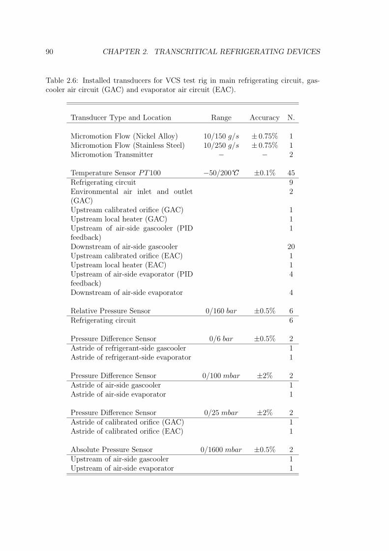
5. transducers, which allow us to perform the measurements and to collect the

feedback signals for controlled devices (pressure transducers, temperature trans-

ducers, mass flow transducers,... );

6. softwares, which allow us to store the measured data, to realize different con-

trol strategies and to analyze on-line/off-line the reliability of performed tests

(acquisition system, flexible control system, post-processing system,... ).

Let us start with the circuit main components. All the heat exchangers of the

refrigerating circuit (gascooler, evaporator and internal heat exchanger) derive from

automotive application. Figures 2.17 and 2.18 report a picture of a one-slab gascooler

and of a one-slab evaporator, respectively. Both gascooler and evaporator are brazed

aluminum heat exchangers with flat microchannel tubes and proper manifolds, which


Figure 2.17: Parallel flow brazed aluminum gascooler with flat microchannel tubes,originally developed for automotive application (Obrist Engineering). The microchan-nel tubes realize a two-pass design. Folded fins without louvers are considered. Ex-ternal sizes for one slab are 615 x 353 x 13 mm (courtesy of Microtecnica s.r.l.).

Figure 2.18: Parallel flow brazed aluminum evaporator with flat microchannel tubes,originally developed for automotive application (Obrist Engineering). The microchan-nel tubes realize a multi-pass design. Folded fins without louvers are considered.External sizes for one slab are 256 x 271 x 42 mm (courtesy of Microtecnica s.r.l.).


realize multi-pass design in order to improve heat transfer effectiveness. Both have

finned air-side surface but the folded fins are smooth, in order to avoid additional

air-side pressure drops due to louvers. This technology allows us to have more than

700 m2 heat transfer surface per 1 m3 core volume, which is close to the current

technological limit for compact heat exchangers. The high working pressure and

favorable heat transfer properties of carbon dioxide enable reduced microchannel

diameters and small refrigerant-side surface areas [20]. This aspect, with regard

to the gascooler, will be discussed later on.

Since the required cooling capacity for the present test rig is greater than that of a

conventional air conditioning system for automotive applications, multi-slab configu-

rations for heat exchangers is needed. In order to evaluate the proper architecture for

the present application, some numerical simulations were run. A numerical code pre-

viously developed was used for this purpose [40] and small changes were introduced

(internal heat exchanger) in order to describe the architectures under investigation.

The numerical code requires detailed geometrical and topological data of both heat

exchangers in order to match real devices and some compressor global performance

data. Both the heat exchangers were discretized by means of a proper number of

subsystems in order to catch effects due to thermo-physical properties variation with

temperature. Finally, the predicted operating conditions and consequent performance

were calculated by means of an iterative procedure, aiming to satisfy the thermal bal-

ance for both heat exchangers. Heat transfer phenomenological correlations taken

from literature were adopted for characterizing heat transfer phenomena and pres-

sure drops. The reliability of the numerical results is guaranteed by an extensive

validation process based on experimental data [40]. In the following, this model is

regarded as the detailed model, previously discussed about integration between ex-


Table 2.5: Numerical simulations for different system architectures: simple architec-

ture A with one-slab gascooler and one-slab evaporator; improved architecture B withtwo-slab gascooler, one-slab evaporator and internal heat exchanger; best architecture

C with two-slab gascooler, two-slab evaporator and internal heat exchanger.

Architecture A B C

Coefficient of performance [−] 0.840 1.434 1.543Refrigerant mass flow rate [kg/s] 0.088 0.056 0.061Cooling capacity [kW ] 3.812 6.426 6.970Mechanical compression power [kW ] 4.538 4.483 4.517Rejected thermal power [kW ] 7.149 10.224 10.526Wasted compressor thermal power [kW ] 0.482 0.642 0.643Wasted discharge line thermal power [kW ] 0.689 0.371 0.404Internal thermal power [kW ] - 3.289 3.890

EvaporatorCooled air mass flow rate [kg/s] 0.334 0.334 0.334Inlet cooled air temperature [ � ] 25.0 25.0 25.0Inlet cooled air humidity ratio [g/kg] 1.950 1.950 1.950Outlet cooled air temperature [ � ] 13.7 6.8 5.0Outlet cooled air humidity ratio [g/kg] 1.947 1.949 1.947

GascoolerCooling air mass flow rate [kg/s] 0.326 0.326 0.326Inlet cooling air temperature [ � ] 30.0 30.0 30.0Outlet cooling air temperature [ � ] 51.3 60.5 61.4

perimental and simulation activity (see Fig. 2.16). The nominal operating conditions

for air-side mass flow rates reported in Tab. 2.4 were assumed.

Three architectures were investigated:

� architecture A, the simplest and most lightweight architecture made of a one-

slab gascooler, a one-slab evaporator, compressor and throttling valve;

� architecture B , an improved architecture which doubles the heat rejection sur-

face by assuming a two-slab gascooler and enables to reach lower enthalpy at


Figure 2.19: Thermodynamic cycles for different system architectures (see Tab. 2.5).

evaporator inlet by adding an internal heat exchanger;

� architecture C, a further improved architecture which doubles the heat transfer

surface at the evaporator too, by assuming a two-slab evaporator.

The numerical results are reported in Tab. 2.5. Fig. 2.19 shows the simulated cy-

cles in the pressure-enthalpy diagram. The first comment is that the simple architec-

ture A does not allow us to satisfy the required cooling capacity (3.8 kW < 6.3 kW ).

The test rig must generate only one third of the cooling capacity of the actual VCS

at aircraft level. Each VCS at aircraft level provides only half (for safety reasons, two

identical systems are expected) of the thermal load assigned to the vapor subsystem

by the hybrid ECS. If we roughly assume that the hybrid ECS divides equally the

thermal load between air and vapor subsystem, the low capacity VCS of the test rig

simulates one twelfth of the actual cooling demand at aircraft level. Two improve-


ments have been considered in order to increase the cooling capacity. Increasing heat

transfer surface of the gascooler allows us to reduce the approach temperature and

consequently to reduce the gascooler outlet enthalpy, which is equal to the evaporator

inlet enthalpy. In the simple architecture A, the evaporator must realize a final super-

heating of the refrigerant in order to avoid liquid suction by the compressor. This

penalizes the heat transfer performance of the evaporator because it forces to work

in a single-phase region, which is characterized by lower heat transfer coefficients.

For this reason, both the improved architectures consider an internal heat exchanger

which enables to realize an evaporation process completely in the two-phase region

(vapor mass fraction is in the range 0.4 − 0.9). It is worth to point out that both

the previous improvements do not directly involve the evaporator, which is still one-

slab. The further architecture C considers a two-slab evaporator. In this case, the

improvement in terms of cooling capacity is smaller than expected. This proves that

the evaporator is a very efficient heat exchanger, which can realize cooling capacities

higher that those it was designed for, but the actual limiting constraint for further

increasing the cooling capacity is the maximum thermal power which can be rejected

by the gascooler. The only benefit of architecture C is an increase of the evapora-

tion temperature, which helps to avoid frosting (see Fig. 2.19). The increase in the

evaporation temperature slightly modifies the suction conditions for the compressor

and this justifies the small discrepancy between the refrigerant mass flow rates of

architecture B and C (see Tab. 2.5). In the experimental test rig, the architecture C

has been implemented.

Once the heat transfer surfaces have been defined, it is possible to select the proper

compressor and the proper rotational speed, which realizes the desired refrigerant

mass flow rate. The selected compressor derives from a mobile application too (bus air


Figure 2.20: Single-stage open two-cylinder piston compressor for carbon dioxide witha swept volume of 110 cm3 and rotational speed range of 500 − 2500 rpm. It is apre-series prototype currently under development (Bock FK −CO2). The eight-poleelectrical motor has a nominal mechanical power of 11 kW and a nominal rotationalspeed of 750 rpm at 50 Hz (courtesy of Microtecnica s.r.l.).

conditioning). Figure 2.20 reports a picture of the installed compressor. Essentially

it is a single-stage two-cylinder piston compressor for carbon dioxide, which is moved

by an external motor. The swept volume is 110 cm3 and the rotational speed range

is 500 − 2500 rpm. Like the previous heat exchangers, it is a pre-series prototype

currently under development too. Taking into account the swept volume, some very

easy calculations allow us to estimate the rotational speed required by architecture

C as included in the range 600 − 800 rpm (it depends on the actual volumetric

efficiency), i.e. close to the lowest allowed speeds. For this reason, the compressor

has been coupled with an eight-pole electrical motor with nominal rotational speed of

750 rpm at 50 Hz and nominal mechanical power of 11 kW . In order to investigate

different rotational speeds, the electrical motor is supplied with an inverter which

enables to tune the electrical frequency in the range 40 − 60 Hz and, consequently,


Figure 2.21: Automatic throttling valve with position feedback control (courtesy ofMicrotecnica s.r.l.).

the rotational speed of the electrical motor in the range 600 − 900 rpm.

In transcritical refrigerating cycles, the high-pressure side is no more related to

the temperature field inside the heat exchanger designed for heat rejection. For this

reason, the high-pressure side becomes a tunable parameter which must be controlled

in order to ensure the best COP. There are many different ways of controlling pres-

sure [20]. The easiest way is to use a throttling valve with an adjustable orifice,

which temporarily changes the balance between compressor mass flow rate and valve

flow rate during transient conditions, in order to vary the high-pressure refrigerant

charge. In fact the pressure in the high-pressure side of the circuit is determinated by

the relationship between refrigerant charge (mass) inside volume and temperature.

Since the total refrigerant charge in the circuit is constant, a refrigerant buffer must

be provided so that the high-pressure charge can be varied without flooding or drying

up the evaporator. In the present application, an automatic throttling valve with po-


Figure 2.22: Refrigerant-side schematic of the experimental test rig (courtesy of Mi-crotecnica s.r.l.).


sitio n feedba ck co ntro l a nd a low-pressure receiv er a s refrig era nt buffer a t ev a po ra to r

o utlet ha v e been a do pted. A picture o f the a uto ma tic v a lv e is repo rted in Fig . 2 .2 1 .

It a llows us to repro duce different co ntro l stra teg ies by simply mo dify ing the so ftwa re

setting s. In pa rticula r, v a ry ing the pressure a t g a sco o ler o utlet (ba ck -pressure wo rk -

ing mo de) in o rder to rea lize the ma x imum CO P a cco rding to the inlet tempera ture

o f the a v a ila ble hea t rejectio n sink , seems a pro mising stra teg y .

The prev io usly discussed ma in co mpo nents a re co llected to g ether in o rder to re-

a lize the refrig era ting circuit. Since the o pera ting pressures fo r tra nscritica l ca rbo n

dio x ide cy cles ca n be v ery hig h (up to 1 4 0 bar), lea k a g e pro blems a re relev a nt. Fo r this

rea so n, a do uble-o g iv e co nnecting techno lo g y (Swa g elo k ) ha s been a do pted beca use

it sho uld ensure the best sea ling . Howev er, the ex perimenta l test rig shows a cha rg e

reductio n due to lea k a g e, which wo uld be una ccepta ble fo r a pra ctica l pro to ty pe wo rk -

ing fo r so me mo nths. Fo rtuna tely this lea k a g e do es no t a ffect the ex perimenta l results

beca use the time needed to perfo rm a n ex perimenta l ca mpa ig n is usua lly sho rter tha n

the time needed to o bserv e a relev a nt cha rg e reductio n g iv ing a lo ss o f ca pa city a nd

CO P .

A co mplete refrig era nt-side schema tic o f the ex perimenta l test rig is repo rted in

Fig . 2 .2 2 . In a dditio n to ma in co mpo nents, so me circuit a ccesso ries, which ena ble the

refrig era ting ma chine to wo rk pro perly , a re needed. The first issue co ncerns the sa fety

dev ices. Two sa fety v a lv es ha v e been a do pted in o rder to a v o id ex plo sio ns a t g a sco o ler

a nd ev a po ra to r a nd a third v a lv e a llows us to by -pa ss the a uto ma tic thro ttling v a lv e,

if it do es no t pro perly wo rk . The co mpresso r wa s eq uipped by the ma nufa cturer

with two integ ra ted sa fety v a lv es a t suctio n a nd discha rg e line. Ano ther issue is

how to intro duce the ca rbo n dio x ide in the refrig era ting circuit. The fill-in a nd the

ex ha ust co nnectio n o f ca rbo n dio x ide were pla ced a t ev a po ra to r inlet. In this wa y , two

88 CHAPTER 2 . TR ANSCR ITICAL R EFR IG ER ATING D EVICES

Figu

re2.23:

Air-sid

esch

ematic

ofth

eex

perim

ental

testrig

(courtesy

ofM

icrotecnica

s.r.l.).

2.3 . DESIGN AND CO NSTRUCTIO N O F THE EXPERIMENTAL TEST RIG 89

heat exchangers (evaporator and internal heat exchanger) are interposed between the

carbon dioxide storing capacity and the compressor. This should reduce the risk of

liquid suction by compressor. Finally an auxiliary heat exchanger (cooling capacity of

100 W at nominal operating conditions) with water as cooling sink has been placed at

gascooler outlet. This device allows us to temporarily tune the approach temperature

without affecting the performance of the internal heat exchanger.

In addition to the refrigerant circuit, the experimental test rig is made by two air

circuits which simulate the thermal load (evaporator air circuit) and the heat rejec-

tion sink (gascooler air circuit) as close as possible to actual operating conditions at

aircraft level. A schematic of both air circuits is reported in Fig. 2.23. The evaporator

is housed in a closed air circuit, while the gascooler is housed in an open air circuit

which can take air from the external environment or partially recirculate it in order

to reduce the energy consumption. B oth the air circuits involve an air fan which

generates the desired mass flow rate, a calibrated orifice for measurement purposes

and a local heater. The local heater of the evaporator air circuit must compensate

the cooling capacity realized by the refrigerating circuit. Since this circuit is prac-

tically closed, the air contained inside the circuit is progressively dehumidified and

the condensed water is extracted by a proper device. This allows us to suppose that,

for steady state conditions, the evaporator air is characterized by very low humidity,

independently of external environment. For this reason, the sensible cooling capacity

largely dominates over the latent cooling capacity and the latter can be practically

neglected for the present application. This peculiarity greatly simplified the design

of experiments because a degree of freedom was removed and the time needed to per-

form an experimental test was shortened. This simplification is acceptable because

some evidences suggest that it is more convenient to assign the whole latent cooling


Table 2.6: Installed transducers for V CS test rig in main refrigerating circuit, gas-cooler air circuit (G AC) and evaporator air circuit (EAC).

Transducer Type and L ocation R ange Accuracy N.

Micromotion Flow (Nickel Alloy) 10/15 0 g /s ± 0.75 % 1Micromotion Flow (Stainless Steel) 10/25 0 g /s ± 0.75 % 1Micromotion Transmitter − − 2

Temperature Sensor P T100 −5 0/200 � ±0.1% 45R efrigerating circuit 9Environmental air inlet and outlet(G AC)

2

Upstream calibrated orifice (G AC) 1Upstream local heater (G AC) 1Upstream of air-side gascooler (PIDfeedback)

1

D ownstream of air-side gascooler 20Upstream calibrated orifice (EAC) 1Upstream local heater (EAC) 1Upstream of air-side evaporator (PIDfeedback)

4

D ownstream of air-side evaporator 4

R elative Pressure Sensor 0/160 bar ±0.5 % 6R efrigerating circuit 6

Pressure D ifference Sensor 0/6 bar ±0.5 % 2Astride of refrigerant-side gascooler 1Astride of refrigerant-side evaporator 1

Pressure D ifference Sensor 0/100 m bar ±2% 2Astride of air-side gascooler 1Astride of air-side evaporator 1

Pressure D ifference Sensor 0/25 m bar ±2% 2Astride of calibrated orifice (G AC) 1Astride of calibrated orifice (EAC) 1

Absolute Pressure Sensor 0/1600 m bar ±0.5 % 2Upstream of air-side gascooler 1Upstream of air-side evaporator 1


capacity to the ACS. In this way, it would be easier to extract the condensed water

and to ensure sanitary conditions by avoiding large wet surfaces. Anyway, it is pos-

sible to estimate the true cooling capacity including latent thermal power by means

of simplified tools (like for example the experimental by-pass factor), which require

to know only the sensible thermal power. The local heater of the gascooler air circuit

allows us to test severe operating conditions due to an increase in cabin temperature.

Both the local heaters are made by electrical resistances and can ensure a maximum

thermal power of 10 kW . Both the air fans are moved by two-pole electrical mo-

tors with nominal rotational speed of 3000 rpm at 50 H z and nominal mechanical

power of 2.3 kW . Both the electrical motors are supplied by inverters which enable

to gradually tune the rotational speed from zero to the maximum value.

The experimental test rig was equipped with some transducers which allowed us

to perform the measurements and to collect the feedback signals for the controlled

devices. A list of the most important transducers is reported in Tab. 2.6. Essentially

the network of transducers has been designed in order to completely characterize the

actual thermodynamic cycle and to estimate the air-side thermal powers involved

in both air circuits. The last feature enables to check the thermal balance of each

heat exchanger and to consequently verify the reliability of the experimental results.

The air inlet temperatures for the gascooler and the evaporator in the respective

air circuits are controlled by means of two independent PID (proportional-integral-

derivative) controllers. The controllers tune the thermal power introduced into air

circuits by local heaters in order to force the air inlet temperatures to become equal

to the user-defined values.

Finally, the experimental test rig has been provided by a data acquisition system

and an on-line post-processing system. The data acquisition system allows us to


Figu

re2.24:

Vap

orC

ycle

Subsy

stemtest

rig(cou

rtesyof

Microtecn

icas.r.l.).


store the measured quantities on 64 independent channels (currently 61 channels are

used) with a frequency of 1 − 2 Hz, which is enough to obtain meaningful results

with regard to heat transfer phenomena. The post-processing system allows us to

check, in every moment during the experimental test, the performances of the actual

refrigerating cycle in terms of cooling capacity and COP, the thermal balance of both

gascooler and evaporator and the time rate of change of meaningful quantities. The

last features are useful to evaluate the effects on cycle performances due to the fill-in

process of carbon dioxide and to establish the reached steady state conditions, which

conclude the test.

A picture of the whole experimental test rig is reported in Fig. 2.24. In the

following, the design of experiments will be discussed and the experimental results

will be analyzed.

2.3.2 Design of experiments and analy sis of the results

The design of experiments deals with the problem of deciding what pattern of ex-

perimental test conditions will best reveal aspects of investigated phenomena and will

best allow us to validate the reduced model [41]. To perform a general experimental

design, a fixed number of discrete values (“ levels” ) for each of a number of variables

(“ factors” ) is selected and then all the possible combinations are experimentally con-

sidered. The goal of the experimental design is to characterize how the investigated

quantity (“ response” ) depends on considered factors. Obviously the same experimen-

tal design can allow us to investigate multiple responses, if they all come from the

same phenomenon. If there are l1 levels for the first variable, l2 for the second,... and

lk for the kth , the complete arrangement of l1× l2× · · · × lk experimental runs is called

an l1 × l2 × · · · × lk factorial design.


For the present application, there are six meaningful factors: the air mass flow

rate at the evaporator inlet Ge; the air mass flow rate at the gascooler inlet Gg; the air

temperature at the evaporator inlet Te; the air temperature at the gascooler inlet Tg;

the working pressure at the gascooler outlet pbp and finally the refrigerant mass flow

rate G. Possible responses are the cooling capacity Φe, the rejected thermal power

Φg and the thermal coefficient of performance TCOP. The TCOP is defined as:

T C O P =Φe

Φg + (Φr h − Φr l) + Φd − Φe

=Φe

Wc − Φc

, (2.1)

where Φr h is the high-pressure-side thermal power due to the internal heat exchanger,

Φr l is the low-pressure-side thermal power due to the internal heat exchanger, Φd is

the thermal power waste of the compressor discharge line, Wc is the mechanical power

absorbed by the compressor and Φc is the compressor thermal power waste. In the

previous definition of TCOP, non-ideal insulation forces to consider additional terms:

Φr h − Φr l ≥ 0, Φd ≥ 0 and Φc ≥ 0. The T C O P differs from the usual coefficient

of performance C O P = Φe/Wc. Taking into account the definition of isoentropic

efficiency %is = W isc /Wc, where W is

c is the isoentropic mechanical power needed to

perform an ideal compression with constant entropy, the following correlation between

TCOP and COP holds:

T C O P =W is

c

Wc − Φc

C O P

%is

. (2.2)

Since in the experimental tests Wc − Φc ≈ W isc , then T C O P ≈ C O P/%is ≥ C O P .

In the design of the experimental test rig, the direct measurement of the mechanical

power need has been neglected because the final goal of the present activity is to pro-

duce some indications about the best architecture for ECS and to produce a reduced

mathematical model, which allows us to characterize the system performance start-

ing from the component performances. For this reason, the available experimental

data on compressor performance are enough to calculate the COP starting from the


Table 2.7: Factorial design for the present application. The design of experimentshas been defined by air-side operating conditions only. It is possible to group the ex-perimental runs characterized by same operating conditions for each heat exchanger.This yields six classes for the evaporator (E1 − 6), with four runs each, and fourclasses for the gascooler (G1 − 4), with six runs each.

Run Air Flow Rate [kg/s] Air Inlet Temperature [ � ] Air-side ClassesEvap. Gasc. Evap. Gasc. Evap. Gasc.

1 0.33 0.33 25 25 E4 G22 0.33 0.33 25 30 E4 G13 0.33 0.33 30 25 E3 G24 0.33 0.33 30 30 E3 G15 0.33 0.27 25 25 E4 G46 0.33 0.27 25 30 E4 G37 0.33 0.27 30 25 E3 G48 0.33 0.27 30 30 E3 G3



TCOP, measured by this experimental test rig.

The number of factors can be reduced. First of all, the refrigerant pressure at the

gascooler outlet should be set equal to the optimal value for the considered approach


Table 2.8: Experimental results for the first set of runs (1−8) defined by the factorialdesign (see Table 2.7). Pressure, temperature and enthalpy (IIF reference state) arereported for seven meaningful points (P1 − 7) which define the refrigerating cycle.See Figure 2.19 for adopted labeling of meaningful cornerstones.

P Run # 1 2 3 4 5 6 7 8

p [±0.7 bar] 87.3 92.1 90.5 94.8 89.9 94.2 93.7 97.91 T [±0.2 � ] 114.1 118.6 118.5 121.7 119.4 122.5 121.7 124.8

h [±0.6 kJ /kg] 534.6 537.5 538.3 539.8 539.8 541.2 540.5 541.9

p [±0.7 bar] 86.1 90.8 89.3 93.5 88.7 92.9 92.3 96.62 T [±0.2 � ] 108.5 113.1 112.9 116.2 113.8 116.8 116.0 119.1

h [±0.6 kJ /kg] 528.2 531.0 531.9 533.5 533.4 534.6 533.9 535.2

p [±0.7 bar] 83.2 87.8 86.4 90.5 85.8 89.9 89.3 93.53 T [±0.1 � ] 37.0 40.1 38.3 41.2 38.9 41.9 40.5 43.5

h [±0.4 kJ /kg] 353.3 359.4 346.4 356.1 359.3 366.3 355.0 362.7

p [±0.7 bar] 82.6 87.2 85.8 89.8 85.1 89.2 88.6 92.74 T [±0.1 � ] 30.8 33.2 32.2 34.9 33.1 35.3 34.5 36.7

h [±0.4 kJ /kg] 285.9 292.9 289.2 299.4 295.2 302.4 298.5 305.4

p [±0.4 bar] 32.8 33.7 34.1 35.4 33.5 34.5 35.1 36.25 T [±0.1 � ] -2.2 -1.3 -0.7 0.6 -1.5 -0.4 0.4 1.4

h [±0.3 kJ /kg] 285.9 292.9 289.2 299.4 295.2 302.4 298.5 305.4

p [±0.4 bar] 31.4 32.3 32.8 34.0 32.1 33.0 33.7 34.76 T [±0.1 � ] -3.8 -2.8 -2.3 -0.9 -3.0 -2.0 -1.2 -0.1

h [±0.3 kJ /kg] 407.5 410.0 419.9 421.9 413.6 414.7 422.3 422.7

p [±0.4 bar] 27.2 28.1 28.6 29.8 28.0 28.9 29.6 30.67 T [±0.1 � ] 18.7 21.0 22.6 25.2 22.2 24.1 25.2 27.2

h [±0.3 kJ /kg] 471.6 473.1 474.2 475.7 474.5 475.5 476.0 477.0


Table 2.9: Experimental results for the second set of runs (9 − 16) defined by thefactorial design (see Table 2.7). Pressure, temperature and enthalpy (IIF referencestate) are reported for seven meaningful points (P1−7) which define the refrigeratingcycle. See Figure 2.19 for adopted labeling of meaningful cornerstones.

P Run # 9 10 11 12 13 14 15 16

p [±0.7 bar] 91.3 97.3 96.5 101.9 96.4 101.3 101.1 106.91 T [±0.2 � ] 107.6 111.8 110.2 115.1 110.9 116.1 115.7 120.3

h [±0.6 kJ/kg] 523.2 524.9 523.1 526.4 524.3 528.1 527.6 530.3

p [±0.7 bar] 89.9 95.8 95.0 100.4 95.0 99.8 99.6 105.32 T [±0.2 � ] 103.3 107.5 106.0 110.9 106.9 111.7 111.3 115.9

h [±0.6 kJ/kg] 518.4 520.0 518.3 521.4 519.7 523.0 522.6 525.2

p [±0.7 bar] 86.4 92.3 91.3 96.7 91.3 96.2 95.8 101.53 T [±0.1 � ] 39.2 42.8 41.2 44.5 42.2 45.4 44.0 47.5

h [±0.4 kJ/kg] 358.3 362.6 351.6 357.2 361.4 367.2 357.0 362.3

p [±0.7 bar] 85.6 91.4 90.4 95.7 90.4 95.3 95.0 100.64 T [±0.1 � ] 26.5 29.0 27.7 29.9 28.3 30.7 29.8 32.2

h [±0.4 kJ/kg] 266.6 272.3 268.4 273.4 270.5 276.2 273.4 279.6

p [±0.4 bar] 31.6 32.6 33.3 34.3 32.5 33.3 34.0 35.05 T [±0.1 � ] -3.7 -2.5 -1.6 -0.6 -2.6 -1.7 -0.9 0.2

h [±0.3 kJ/kg] 266.6 272.3 268.4 273.4 270.5 276.2 273.4 279.6

p [±0.4 bar] 30.0 31.0 31.7 32.6 30.9 31.6 32.3 33.36 T [±0.1 � ] -5.5 -4.3 -3.5 -2.5 -4.5 -3.6 -2.8 -1.7

h [±0.3 kJ/kg] 363.4 365.7 372.7 374.0 363.8 366.9 375.0 377.6

p [±0.4 bar] 24.9 25.9 26.4 27.3 25.8 26.5 27.1 28.07 T [±0.1 � ] -1.5 0.6 1.6 4.2 -0.4 2.9 4.5 7.1

h [±0.3 kJ/kg] 450.5 451.4 451.7 453.5 450.2 453.4 454.4 456.2


Table 2.10: Experimental results for the third set of runs (17 − 24) defined by thefactorial design (see Table 2.7). Pressure, temperature and enthalpy (IIF referencestate) are reported for seven meaningful points (P1−7) which define the refrigeratingcycle. See Figure 2.19 for adopted labeling of meaningful cornerstones.

P Run # 17 18 19 20 21 22 23 24

p [±0.7 bar] 88.5 92.1 91.5 95.9 91.4 95.1 95.1 99.21 T [±0.2 � ] 123.1 127.3 126.4 130.4 128.2 131.1 130.1 133.3

h [±0.6 kJ/kg] 545.6 548.6 547.9 550.4 550.2 551.8 550.5 552.3

p [±0.7 bar] 87.4 91.0 90.4 94.7 90.2 93.8 93.8 97.92 T [±0.2 � ] 116.7 120.8 120.0 123.9 121.6 124.6 123.7 126.9

h [±0.6 kJ/kg] 538.0 541.0 540.4 542.7 542.6 544.1 543.0 544.7

p [±0.7 bar] 84.9 88.4 87.8 92.1 87.6 91.1 91.1 95.13 T [±0.1 � ] 37.7 40.1 38.6 41.5 39.6 42.2 41.0 43.8

h [±0.4 kJ/kg] 349.0 355.8 340.9 349.8 354.6 362.3 349.9 358.1

p [±0.7 bar] 84.3 87.8 87.2 91.4 87.0 90.5 90.4 94.44 T [±0.1 � ] 34.7 36.9 36.0 38.5 36.6 38.7 38.1 40.5

h [±0.4 kJ/kg] 309.5 319.2 312.7 322.6 320.5 327.7 322.2 330.1

p [±0.4 bar] 33.3 34.2 34.6 35.6 34.0 35.0 35.6 36.65 T [±0.1 � ] -1.7 -0.7 -0.2 0.9 -0.9 0.2 0.9 1.9

h [±0.3 kJ/kg] 309.5 319.2 312.7 322.6 320.5 327.7 322.2 330.1

p [±0.4 bar] 31.4 32.2 32.6 33.5 32.0 32.9 33.5 34.46 T [±0.1 � ] -3.9 -3.0 -2.5 -1.5 -3.1 -2.1 -1.5 -0.5

h [±0.3 kJ/kg] 444.9 449.1 456.9 459.5 451.7 452.4 458.6 459.9

p [±0.4 bar] 27.3 28.1 28.5 29.4 28.1 29.0 29.5 30.47 T [±0.1 � ] 28.3 30.5 30.8 33.2 30.6 32.6 32.9 35.1

h [±0.3 kJ/kg] 482.4 483.9 483.8 485.3 484.0 485.2 485.0 486.5


temperature in order to realize the maximum COP. Moreover, the refrigerant mass

flow rate is mainly a result of the compressor rotational speed because suction cannot

change too much for the considered operating conditions and the same holds for the

volumetric efficiency according to the results of specific tests on the compressor alone.

For these reasons, both previous quantities will be investigated numerically by means

of the reduced mathematical model. Only the air-side quantities will be considered

for the experimental design. The minimum number of levels (2) will be considered for

all factors, with the exception of the air flow rate at the evaporator inlet where 3 levels

will be considered because the range of this parameter is wider (see Tab. 2.4). The

previous assumptions define a 3 × 2 × 2 × 2 factorial design, which requires 24 runs.

The experimental design is reported in Tab. 2.7. For a given design, it is possible to

extract an experimental sub-design by considering a proper sub-set of factors. For

example, let us suppose to fix all the factors related to the evaporator, i.e. Ge and

Te. This defines a 2 × 2 factorial sub-design with 4 runs for the residual factors, i.e.

Gg and Tg. Since the number of runs of the whole experimental design is greater

than that of the sub-design (24 > 4 in the reported example), it is possible to use

these additional data for statistically estimating the effects due to the factors kept

constant for each sub-design. This issue will be discussed later on when dealing with

the reduced model. The sub-designs for both evaporator and gascooler are reported

in Tab. 2.7, too.

In order to characterize the thermodynamic cycle, let us consider the following

components only: discharge line (d subscript), gascooler (g subscript), high-pressure-

side internal heat exchanger (rh subscript), throttling valve (v subscript), evaporator

(e subscript), low-pressure-side internal heat exchanger (rl subscript) and compres-

sor (c subscript). Consequently let us define the following cornerstone labels (see


Table 2.11: Comparison between air-side (AS) and refrigerant-side (RS) measure-ments. The thermal balance for both the heat exchangers is verified by means of therelative percentage error (R), defined as R = (AS − RS)/RS × 100. The air-sidemeasurements have not been performed for the third set of runs (17 − 24).

Thermal PowerGascooler [kW ] Evaporator [kW ] Internal TCOP

Air-Side Refr.-Side R Air-Side Refr.-Side R [kW ] [−]

1 10.88 10.45 3.97 8.31 7.27 12.50 3.83 1.932 10.69 10.46 2.15 8.11 7.13 12.00 3.85 1.823 11.83 11.39 3.75 9.41 8.02 14.78 3.34 2.044 11.52 11.28 2.12 8.99 7.78 13.40 3.42 1.915 10.83 10.43 3.73 8.19 7.09 13.34 3.65 1.816 10.57 10.35 2.06 7.82 6.91 11.65 3.75 1.717 11.59 11.25 2.94 9.10 7.78 14.51 3.38 1.928 11.31 11.15 1.39 8.78 7.58 13.73 3.51 1.81

9 11.87 11.16 6.04 7.20 6.74 6.81 6.06 1.3310 11.77 11.31 3.91 7.06 6.71 5.19 6.16 1.2711 12.89 12.32 4.44 8.38 7.71 8.69 5.83 1.4612 12.77 12.40 2.92 8.01 7.58 5.69 6.03 1.3813 11.80 11.41 3.33 7.17 6.73 6.56 6.22 1.2614 11.57 11.32 2.16 6.85 6.59 3.81 6.29 1.2115 12.65 12.31 2.73 8.12 7.54 7.64 5.90 1.3916 12.54 12.38 1.21 7.90 7.44 6.21 5.99 1.32

Figs. 2.19 and 2.22):

1. compressor outlet and discharge line inlet (P1),

2. discharge line outlet and gascooler inlet (P2),

3. gascooler outlet and high-pressure-side internal heat exchanger inlet (P3),

4. high-pressure-side internal heat exchanger outlet and throttling valve inlet (P4),

5. throttling valve outlet and evaporator inlet (P5),

6. evaporator outlet and low-pressure-side internal heat exchanger inlet (P6),

7. low-pressure-side internal heat exchanger outlet and compressor inlet (P7).

The experimental data in terms of pressure, temperature and specific enthalpy for

2.3. DESIGN AND CONSTRUCTION OF THE EXPERIMENTAL TEST RIG101

the cornerstones of the thermodynamic cycle are reported in Tab. 2.8 for runs #1−8,

in Tab. 2.9 for runs #9 − 16 and in Tab. 2.10 for runs #17 − 24 of the experimental

design. It was not possible to repeat the experimental tests a number of times suitable

for evaluating the statistical scattering due to experimental inaccuracies. For this

reason, the previous data are not provided with their error bars, but at least the

accuracy of the instrument was considered. Moreover it was not possible to ensure

exactly the same refrigerant charge during all the experimental tests because of the

leakage problems. This point will be discussed better in Chapter 5. In order to reduce

the effects of the refrigerant charge on the measurements, the experimental procedure

included a preliminary phase during which the refrigerant mass was carefully regulated

in order to reproduce a fixed reference cycle. To reproduce the reference cycle means

that the pressure and specific enthalpy values for the seven cornerstones (P1 − 7),

shown in Figs. 2.19 and 2.22, differ from the reference values for less than 2%. Even

though this way of tuning the refrigerant charge is indirect, it allowed to verify the

unperturbated reference cycle before investigating each test of the experimental plan.

Taking into account the previous data, it is possible to calculate the cooling capac-

ity, the rejected thermal power and the TCOP for each experimental run. Since both

air circuits are provided with temperature transducers (the effects due to moisture

content can be neglected), it is possible to verify the thermal balance for both main

heat exchangers. The post-processed experimental results are reported in Tab. 2.11.

The difference between air-side and refrigerant-side measurements with regard to

transferred thermal power are very good for the gascooler. In this case, the relative

error on the thermal balance is less than 6%. Unfortunately the same error for the

evaporator is much higher and it can be equal to 15% as maximum value. This error

is not due to the simplifying assumption of neglecting the latent thermal power. In


fact this error means that the air-side estimation overestimates the transferred ther-

mal power. Since only the sensible thermal power is measured, at most the air-side

estimation should be smaller than refrigerant-side one, which involves both sensible

and latent thermal power. Moreover the error is a monotonic increasing function of

the air mass flow rate at the evaporator: the average error is around 6% for 0.27 kg/s

and 13% for 0.33 kg/s. On the other hand, the refrigerant-side measurements for

the evaporator are quite critical because, for all the experimental runs, a two-phase

flow exists at the evaporator inlet and, for the majority of the experimental runs,

the same holds at the evaporator outlet too. In this case, temperature and pres-

sure data do not allow us to estimate the inlet and outlet void fraction. Hence the

refrigerant-side measurements for the evaporator are indirect. The evaporator inlet

enthalpy is assumed equal to the throttling valve inlet enthalpy and the evaporator

outlet is estimated by means of the outlet enthalpy of the low-pressure-side internal

heat exchanger and an extrapolated efficiency (95%) for the last component. The

extrapolated efficiency is based on experimental data for the internal heat exchanger

only. Anyway, despite the inaccuracies of the refrigerant-side measurements, it is

plausible to trust them more because the estimated maximum error is close to 10%,

which is lower than that on thermal balance. For this reason, it is plausible to sup-

pose that the error is mainly due to an air leakage in the evaporator air circuit (EAC)

between the measurement section for the air mass flow rate and the evaporator inlet.

This means that a slightly reduced fraction of the measured air mass flow rate really

passes through the evaporator and it is involved in the heat transfer process.

In the derivation of the reduced model, only the refrigerant-side data will be

considered. Anyway, the described procedure is general and it can be applied to

multiple experimental designs in order to find statistically meaningful results.

2.4 . REDUCED MODEL 103

2.4 Reduced model

In this section, a reduced mathematical model which interpolates the experimental

data will be developed. In this case, the reduction technique is essentially a regression

method (see Fig. 2.16).

2.4.1 Design of the reduced model

First of all, the physical quantities must be properly made dimensionless in order

to reduce the round-off errors. Let us define η = h/h0 the dimensionless enthalpy,

π = p/p0 the dimensionless pressure and σ = G/G0 the dimensionless refrigerant

mass flow rate. In the same way, we can proceed for the air-side quantities. Let

us define θ = Ta/T0 the dimensionless air inlet temperature and ς = Ga/G0 the

dimensionless mass flow rate. The subscript will identify the generic component,

according to the nomenclature introduced in the previous section. The input data for

the model are the following user-defined quantities: ςeu, ςg

u, θeu, θg

u, σu and π4,u, which

is the set point of the back-pressure throttling valve. The output data are the cooling

capacity Φe = G0 h0 σ(η6 − η5), the rejected thermal power Φg = G0 h0 σ(η2 − η3), the

high-pressure-side internal thermal power Φrh = G0 h0 σ(η3 − η4), the low-pressure-

side internal thermal power Φrl = G0 h0 σ(η7 − η6), the thermal power waste of the

discharge line Φd = G0 h0 σ(η1 − η2) and finally the TCOP, calculated by means

of Eq. (2.1). As it is evident by looking at the previous definitions, the reduced

model must predict the cornerstones of the thermodynamic cycle in order to properly

calculate all the output data.

As previously discussed, for a given experimental design, it is possible to extract an

experimental sub-design by considering a proper sub-set of factors. For example, let us


consider a generic component k, which is characterized by some factors with regard to

air-side condition, and let us suppose to keep them constant. All the residual factors

allow us to define a factorial sub-design, which requires Nk runs. Since the number of

runs for the experimental sub-design is smaller than that for full experimental design

Nk ≤ N , then Mk = N/Nk multiple sub-designs exist. It is possible to use the results

due to different sub-designs in order to statistically estimate the effects of the factors

kept constant for each sub-design. If the component does not involve air circuits and

there is no need to characterize the air-side condition, then Nk = N and Mk = 1.

The enthalpy difference and the pressure difference for the generic k component

contained between the cornerstone i and the cornerstone i + 1 can be approximated

as linear combinations of the inlet state i and the refrigerant mass flow rate, namely:

ηi − ηi+1 = αkηηi + αk

π πi + αkσ σu + αk

0, (2.3)

πi − πi+1 = βkηηi + βk

π πi + βkσ σu + βk

0 , (2.4)

where αkη, αk

σ, αk0 are the coefficients of the linear approximation for the enthalpy

difference and similarly βkη , βk

σ, βk0 are the coefficients of the linear approximation

for the pressure difference. These coefficients can be obtained by two recursive least

square fittings of the experimental data.

In the following, only the coefficients for the enthalpy difference will be reported

but it is easy to proceed in a similar way for the pressure difference. Some auxiliary

coefficients will be derived by a first least square fitting of the experimental data for

the generic m sub-design. This yields:

αk, mη

Nk∑

n= 1

(ηni )2 + αk, m

π

Nk∑

n= 1

ηni πn

i + αk, mσ

Nk∑

n= 1

ηni σ + αk, m

0

Nk∑

n= 1

ηni =

Nk∑

n= 1

ηni

(

ηni − ηn

i+1

)

, (2.5)

2.4. REDUCED MODEL 105

αk, mη

Nk∑

n=1

πni ηn

i + αk, mπ

Nk∑

n=1

(πni )2 + αk, m

σ

Nk∑

n=1

πni σ + αk, m

0

Nk∑

n=1

πni =

Nk∑

n=1

πni

(

ηni − ηn

i+1

)

, (2.6)

αk, mη

Nk∑

n=1

σηni + αk, m

π

Nk∑

n=1

σπni + αk, m

σ

Nk∑

n=1

(σ)2 + αk, m0

Nk∑

n=1

σ =

Nk∑

n=1

σ(

ηni − ηn

i+1

)

, (2.7)

αk, mη

Nk∑

n=1

ηni + αk, m

π

Nk∑

n=1

πni + αk, m

σ

Nk∑

n=1

σ + αk, m0 Nk =

Nk∑

n=1

(

ηni − ηn

i+1

)

. (2.8)

The previous equations define a linear system of equations in the variables αk, mη ,

αk, mπ , αk, m

σ and αk, m0 . It is easy to verify that the matrix involved in this system

of equations is the Vandermonde’s matrix, which is generally characterized by high

condition numbers. For this reason, searching for a good solution of the previous

system by means of iterative techniques can be quite difficult. However for the present

application, the small number of variables and the small number of experimental data

allowed to easily solve the system by means of a direct technique.

Therefore a second least square fitting is performed on the previous interpolation

coefficients themselves by considering all the Mk experimental sub-designs. In this

case, the interpolation variables are those needed to characterize the air-side condi-

tions. In the following, only the procedure for the coefficient αk, mη is reported but the

same must be performed for αk, mπ , αk, m

σ and αk, m0 too. This yields:

γkς , η

Mk∑

m=1

(

ςkm

)2+ γk

θ , η

Mk∑

m=1

ςkmθk

m + γk0, η

Mk∑

m=1

ςkm =

Mk∑

m=1

ςkmαk, m

η , (2.9)

γkς , η

Mk∑

m=1

θkmςk

m + γkθ , η

Mk∑

m=1

(

θkm

)2+ γk

0, η

Mk∑

m=1

θkm =

Mk∑

m=1

θkmαk, m

η , (2.10)


γkς, η

Mk∑

m=1

ςkm + γk

θ, η

Mk∑

m=1

θkm + γk

0, η Mk =

Mk∑

m=1

αk, mη . (2.11)

The previous equations define a linear system of equations in the variables γkς, η, γk

θ, η

and γk0, η. The matrix involved in this system of equations is again the Vandermonde’s

matrix, but the same simplifying conditions, which have been previously discussed,

hold. Finally the interpolating coefficient αkη involved in Eq. (2.3) can be derived by

considering the user-defined input data, namely:

αkη = γk

ς, η ςku + γk

θ, η θku + γk

0, η. (2.12)

This means that a first set of the user-defined input data, i.e. ςeu, ςg

u, θeu and θg

u, are

involved in the calculation of the interpolating coefficients for the evaporator and the

gascooler. If the component does not involve air circuits and there is no need to

characterize the air-side condition, then αk, mη = αk

η = γk0, η.

The Eqs. (2.3, 2.4) can be written for all the components and they finally define

a linear system of equations, which allows us to calculate all the cornerstones and

consequently the thermodynamic cycle. This system of equations is:

[

Aη Aπ

Bη Bπ

] {

xη

xπ

}

+

{

x0

η

x0

π

}

= 0, (2.13)

where the previous vectors are:

xη = {η1, η2, η3, η4, η5, η6, η7}T , (2.14)

xπ = {π1, π2, π3, π4, π5, π6, π7}T , (2.15)

x0

η ={

αdσσ

u + αd0, αg

σσu + αg

0, αrhσ σu + αrh

0 , 0,

αeσσ

u + αe0, αrl

σ σu + αrl0 , αc

σσu + αc

0

}T, (2.16)

x0

π ={

βdσσ

u + βd0 , βg

σσu + βg

0 , βrhσ σu + βrh

0 , πu4 ,

βeσσ

u + βe0, βrl

σ σu + βrl0 , βc

σσu + βc

0

}T, (2.17)


and the previous matrices are:

Aη =

αdη − 1 +1 0 0 0 0 00 αg

η − 1 +1 0 0 0 00 0 −1 +1 0 αrh

η 00 0 0 −1 +1 0 00 0 0 0 αe

η − 1 +1 00 0 0 0 0 αrl

η − 1 +1+1 0 0 0 0 0 αc

η − 1

, (2.18)

Aπ =

αdπ 0 0 0 0 0 00 αg

π 0 0 0 0 00 0 0 0 0 αrh

π 00 0 0 0 0 0 00 0 0 0 αe

π 0 00 0 0 0 0 αrl

π 00 0 0 0 0 0 αc

π

, (2.19)

Bη =

βdη 0 0 0 0 0 00 βg

η 0 0 0 0 00 0 0 0 0 βrh

η 00 0 0 0 0 0 00 0 0 0 βe

η 0 00 0 0 0 0 βrl

η 00 0 0 0 0 0 βc

η

, (2.20)

Bπ =

βdπ − 1 +1 0 0 0 0 00 βg

π − 1 +1 0 0 0 00 0 −1 +1 0 βrh

π 00 0 0 −1 0 0 00 0 0 0 βe

π − 1 +1 00 0 0 0 0 βrl

π − 1 +1+1 0 0 0 0 0 βc

π − 1

. (2.21)

In order to define the previous system of equations, some simplifying hypotheses have

been considered. The back-pressure throttling valve has been described in an idealized

way by assuming η4 = η3 and π4 = π4, u. Moreover the interpolating expressions for

the internal heat exchanger differ from the other components. Since the internal

thermal powers on both sides are very similar to each other (they can differ for

non-ideal insulation only), it is better that both of them are functions of the same

variables. The efficiency of the internal heat exchanger highly depends on the nature

(single-phase or two-phase) of the fluid flow in the low-pressure-side. Hence it is


better to use the inlet conditions for the low-pressure part for interpolating both the

transformations (3-4 and 6-7) realized by the internal heat exchanger because, in this

way, it is easier to take into account the fact that the low-pressure-side fluid flow is

single-phase or two-phase. For this reason, the enthalpy and pressure difference for

the high-pressure part are expressed as linear functions of the inlet conditions for the

low-pressure part.

2.4.2 Numerical results

First of all, the numerical results due to the reduced model have been compared

with the original experimental data in order to verify that the two recursive least

square fittings do not affect the reliability of the predictions. The comparison is re-

ported in Tab. 2.12 and it shows a very good match for the most important quantities.

In fact the discrepancy between the experimental data and the numerical results is

very small for the cooling capacity (−4.0 % ≤ R ≤ +4.1 %) and for the rejected

thermal power (−1.6 % ≤ R ≤ +3.6 %), while it is a bit higher for the TCOP

(−9.5 % ≤ R ≤ +9.2 %). The reason is due to the fact that the TCOP involves a

ratio of estimated quantities and it is very sensitive to inaccuracies. The accuracy is

also poor for the transferred thermal power due to the internal heat exchanger. In

this case, it is difficult to accurately predict thermal powers which are much smaller

that those due to the main heat exchangers. Anyway the effects on the whole device

performances due to the last inaccurate estimation of the internal thermal power are

very modest. Recalling that the numerical results are due to a simple data fitting,

the comparison is reasonable and the reduced model will be used for analysing the

effects due to the VCS installation strategy. The evaporator can be installed:

� after the mixing point (AM) between recirculated air taken from the cabin and

the refrigerated air due to the 3WM-ACS (see sketched lines in Fig. 2.6) and


Table 2.12: Comparison between experimental and numerical results due to reducedmodel for the considered factorial design (see Table 2.7). For each thermal power,three values are reported which are respectively the experimental datum (E), thenumerical result due to the reduced model (M) and the relative percentage error (R),defined as R = (E − M)/M × 100.

Thermal PowerGascooler [kW ] Evaporator [kW ] Internal [kW ] TCOP [−]E M R E M R E M E M R

1 10.45 10.54 0.9 7.27 7.06 -2.8 3.83 3.42 1.93 1.75 -9.52 10.46 10.84 3.6 7.13 7.19 0.8 3.85 2.34 1.82 1.71 -5.93 11.39 11.26 -1.1 8.02 7.80 -2.8 3.34 3.30 2.04 1.93 -5.44 11.28 11.35 0.7 7.78 7.66 -1.6 3.42 3.50 1.91 1.78 -6.65 10.43 10.71 2.7 7.09 7.16 0.9 3.65 2.51 1.81 1.74 -3.76 10.35 10.57 2.1 6.91 6.91 -0.0 3.75 2.42 1.71 1.64 -4.17 11.25 11.17 -0.7 7.78 7.58 -2.6 3.38 3.44 1.92 1.81 -5.78 11.15 11.01 -1.3 7.58 7.30 -3.7 3.51 3.30 1.81 1.69 -6.5

9 11.16 11.03 -1.1 6.74 6.65 -1.3 6.06 6.72 1.33 1.32 -1.010 11.31 11.52 1.8 6.71 6.98 4.1 6.16 6.08 1.27 1.34 5.611 12.32 12.15 -1.3 7.71 7.43 -3.6 5.83 7.31 1.46 1.37 -6.312 12.40 12.52 1.0 7.58 7.68 1.4 6.03 6.14 1.38 1.39 0.913 11.41 11.47 0.5 6.73 6.91 2.8 6.22 6.28 1.26 1.32 4.914 11.32 11.34 0.1 6.59 6.79 3.0 6.29 5.64 1.21 1.30 7.115 12.31 12.39 0.7 7.54 7.66 1.6 5.90 5.90 1.39 1.42 2.216 12.38 12.34 -0.4 7.44 7.47 0.3 5.99 5.27 1.32 1.34 1.9

17 10.75 10.85 0.9 7.91 7.78 -1.6 1.93 2.47 2.20 2.15 -2.118 10.73 10.89 1.5 7.55 7.76 2.8 1.99 2.06 2.01 2.11 5.019 11.73 11.57 -1.3 8.63 8.28 -4.0 1.43 2.27 2.29 2.16 -5.720 11.62 11.72 0.9 8.24 8.37 1.5 1.56 1.64 2.10 2.15 2.021 10.80 10.73 -0.6 7.52 7.70 2.3 1.87 1.95 1.98 2.16 9.022 10.69 10.56 -1.3 7.23 7.42 2.8 2.04 1.95 1.84 2.01 9.223 11.62 11.49 -1.1 8.25 8.16 -1.2 1.54 1.92 2.09 2.10 0.324 11.50 11.32 -1.6 7.96 7.87 -1.1 1.68 1.78 1.96 1.96 0.0


Figu

re2.25:

Num

ericalresu

ltsdue

tored

uced

model:

effects

ofrefrigeran

tm

assflow

ratean

dset

poin

tof

back

-pressu

revalve

with

evaporator

installed

afte

rth

em

ixin

gpoin

t(see

Fig.

2.6).T

he

air-side

condition

sfor

the

evaporator

areG

e=

0.47kg/s

(max

imum

value)

and

Tea=

20

�

(min

imum

value),

while

those

forth

egasco

olerare

Ge=

0.30kg/s

and

Tea=

27

�

.


Fig

ure

2.26

:N

um

eric

alre

sults

due

tore

duce

dm

odel

:eff

ects

ofre

frig

eran

tm

ass

flow

rate

and

set

poi

nt

ofbac

k-p

ress

ure

valv

ew

ith

evap

orat

orin

stal

led

befo

re

the

mix

ing

poi

nt

(see

Fig

.2.

6).

The

air-

side

conditio

ns

for

the

evap

orat

orar

eG

e=

0.27

kg/s

(min

imum

valu

e)an

dT

e a=

30

(max

imum

valu

e),w

hile

thos

efo

rth

ega

scool

erar

eG

e=

0.30

kg/s

and

Te a=

27

.


this would ensure the maximum air mass flow rate (roughly Gea = 0.47 kg/s

for the low capacity tes rig) but the minimum air inlet temperature (roughly

T ea = 20 ! ) or

" before the mixing point (BM) in the recirculation air duct which takes air from

the cabin (see continuous lines in Fig. 2.6) and this would ensure the maximum

air inlet temperature (roughly T ea = 30 ! ) but the minimum air mass flow rate

(roughly Gea = 0.27 kg/s for the low capacity test rig).

Both previous configurations have been investigated and the numerical results

for the cooling capacity, the rejected thermal power, the internal thermal power and

the TCOP are reported in Figs. 2.25 and 2.26. The asterisks denote the actual ex-

perimental measurements. The air-side conditions for the gascooler are the same in

both cases. The effects of the refrigerant mass flow rate and the set point of the

back-pressure valve are investigated too. It is easy to verify that the previous results

are substantially identical for both configurations. This seems somehow to prove the

idea that the two configurations are equivalent, but they are not. In fact, the real

systems do not work with a fixed refrigerant mass flow rate. In the electrified air-

craft architecture, the compressor will be powered by an electrical motor controlled

by an inverter and the feedback will be on the rotational speed. For this reason, the

effective refrigerant mass flow rate can change according to the density of the actual

suction condition. The same holds for the reported experimental design. Consid-

ering Tabs. 2.8, 2.9 and 2.10, it is easy to verify that the suction density decreases

when the air mass flow rate at the evaporator increases. In fact, high air mass flow

rate at the evaporator enhances the efficiency of the evaporator and consequently

the super-heating too. Working with a fixed rotational speed leads to a consequent

reduction of the refrigerant mass flow rate. As shown in the bottom-right sub-plots

2.5 . CONCLUSIONS 113

of Figs. 2.25 and 2.26, reducing the refrigerant mass flow rate for a given set point of

the back-pressure valve increases the TCOP. Unfortunately, as shown in the top-left

sub-plots in the same figures, this reduces the cooling capacity too. For this reason,

the after-mixing (AM) installation strategy (see Fig. 2.6) for the evaporator is prefer-

able for reducing the energy consumption, but this could force to consider larger heat

exchangers. Actually the air mass flow rate at the evaporator does not directly affect

the performances of the transcritical cycle but it reduces the suction density, conse-

quently the refrigerant mass flow rate and this is enough to increase the coefficient of

performance.

2.5 Conclusions

In this section, the main outlines for the design of an experimental test rig which

enables us to characterize the thermal performances of a refrigerating device based

on a carbon dioxide transcritical cycle have been discussed. The final goal of this

experimental test rig is to prove that the trascritical device can properly match the

required specifications in order to be integrated with a conventional air-cycle machine

and to realize in this way a hybrid air conditioning system for airborne application.

The experimental results are encouraging because the expected performances have

been realized. This means that, in principle, the transcritical thermodynamic cycle

can properly work for this application. However from the technological point of view,

some problems still remain. First of all, the leakage problems of this prototype, which

complicated the management of the experimental tests because they did not allow us

to work with the same carbon dioxide charge for the whole experimental plan, would

be completely unacceptable for a standard market device. Obviously this problem

can be mitigated by considering better technologies for the gaskets, but this could


complicate the installation/ maintenance of these devices in comparison with usual air-

cycle machines. Secondly, automotive prototypes have been considered as components

for the discussed exercise, but they are not the more lightweight and ultra-compact

solutions, as required by airborne standards. Large opportunities of optimization in

this direction exist, particularly for the compressor. Even though some compressors

designed for other applications dealing with higher pressures exist (see, for example,

methane compressors used in automotive applications, which are characterized by

discharge pressures up to 200 bar), up to now the lubricants for carbon dioxide are

still in their infancy and this substantially hinders the development of reliable carbon

dioxide compressors.

Discussing the design of the experimental test rig, the importance of the thermal

rejection phase for improving the performances of the transcritical cycle has been

pointed out and consequently the importance of the gascooler too. Finned compact

gascoolers made of flat extruded aluminum tubes with internal mini/ micro-channels

constitute a promising technology and the optimization of this type of heat exchangers

is therefore one of the main research goal for the development of refrigerating systems

operated with carbon dioxide. For this reason, these compact heat exchangers will

be analyzed more extensively in the next chapter.

Date post:	21-Jul-2020
Category:	Documents
Upload:	others
View:	1 times
Download:	0 times

Chapter 2 T ranscritical refrigerating devices · tion of greenhouse gases in the Earth’s...

Documents