Chapter 2 The Solow Growth Model (and a look ahead) 2.1 Centralized Dictatorial Allocations • In this section, we start the analysis of the Solow model by pretending that there is a dictator, or social planner, that chooses the static and intertemporal allocation of resources and dictates that allocations to the households of the economy We will later show that the allocations that prevail in a decentralized competitive market environ- ment coincide with the allocations dictated by the social planner. 2.1.1 The Economy, the Households and the Dictator • Time is discrete, t ∈ {0, 1, 2, ...}. You can think of the period as a year, as a generation, or as any other arbitrary length of time. • The economy is an isolated island. Many households live in this island. There are 9
Transcript
Chapter 2
The Solow Growth Model (and a look
ahead)
2.1 Centralized Dictatorial Allocations
• In this section, we start the analysis of the Solow model by pretending that there is
a dictator, or social planner, that chooses the static and intertemporal allocation of
resources and dictates that allocations to the households of the economy We will later
show that the allocations that prevail in a decentralized competitive market environ-
ment coincide with the allocations dictated by the social planner.
2.1.1 The Economy, the Households and the Dictator
• Time is discrete, t ∈ {0, 1, 2, ...}. You can think of the period as a year, as a generation,
or as any other arbitrary length of time.
• The economy is an isolated island. Many households live in this island. There are
9
George-Marios Angeletos
no markets and production is centralized. There is a benevolent dictator, or social
planner, who governs all economic and social affairs.
• There is one good, which is produced with two factors of production, capital and labor,
and which can be either consumed in the same period, or invested as capital for the
next period.
• Households are each endowed with one unit of labor, which they supply inelasticly to
the social planner. The social planner uses the entire labor force together with the
accumulated aggregate capital stock to produce the one good of the economy.
• In each period, the social planner saves a constant fraction s ∈ (0, 1) of contemporane-
ous output, to be added to the economy’s capital stock, and distributes the remaining
fraction uniformly across the households of the economy.
• In what follows, we let Lt denote the number of households (and the size of the labor
force) in period t, Kt aggregate capital stock in the beginning of period t, Yt aggregate
output in period t, Ct aggregate consumption in period t, and It aggregate investment
in period t. The corresponding lower-case variables represent per-capita measures: kt =
Kt/Lt, yt = Yt/Lt, it = It/Lt, and ct = Ct/Lt.
2.1.2 Technology and Production
• The technology for producing the good is given by
Yt = F (Kt, Lt) (2.1)
where F : R2+ → R+ is a (stationary) production function. We assume that F is
continuous and (although not always necessary) twice differentiable.
10
Lecture Notes
• We say that the technology is “neoclassical” if F satisfies the following properties
1. Constant returns to scale (CRS), or linear homogeneity:
F (µK, µL) = µF (K,L), ∀µ > 0.
2. Positive and diminishing marginal products:
FK(K,L) > 0, FL(K,L) > 0,
FKK(K,L) < 0, FLL(K,L) < 0.
where Fx ≡ ∂F/∂x and Fxz ≡ ∂2F/(∂x∂z) for x, z ∈ {K,L}.
3. Inada conditions:
limK→0
FK = limL→0
FL =∞,
limK→∞
FK = limL→∞
FL = 0.
• By implication, F satisfies
Y = F (K,L) = FK(K,L)K + FL(K,L)L
or equivalently
1 = εK + εL
where
εK ≡∂F
∂K
K
Fand εL ≡
∂F
∂L
L
F
Also, FK and FL are homogeneous of degree zero, meaning that the marginal products
depend only on the ratio K/L.
And, FKL > 0, meaning that capital and labor are complementary.
Finally, all inputs are essential: F (0, L) = F (K, 0) = 0.
11
George-Marios Angeletos
• Technology in intensive form: Let
y =Y
Land k =
K
L.
Then, by CRS
y = f(k) (2.2)
where
f(k) ≡ F (k, 1).
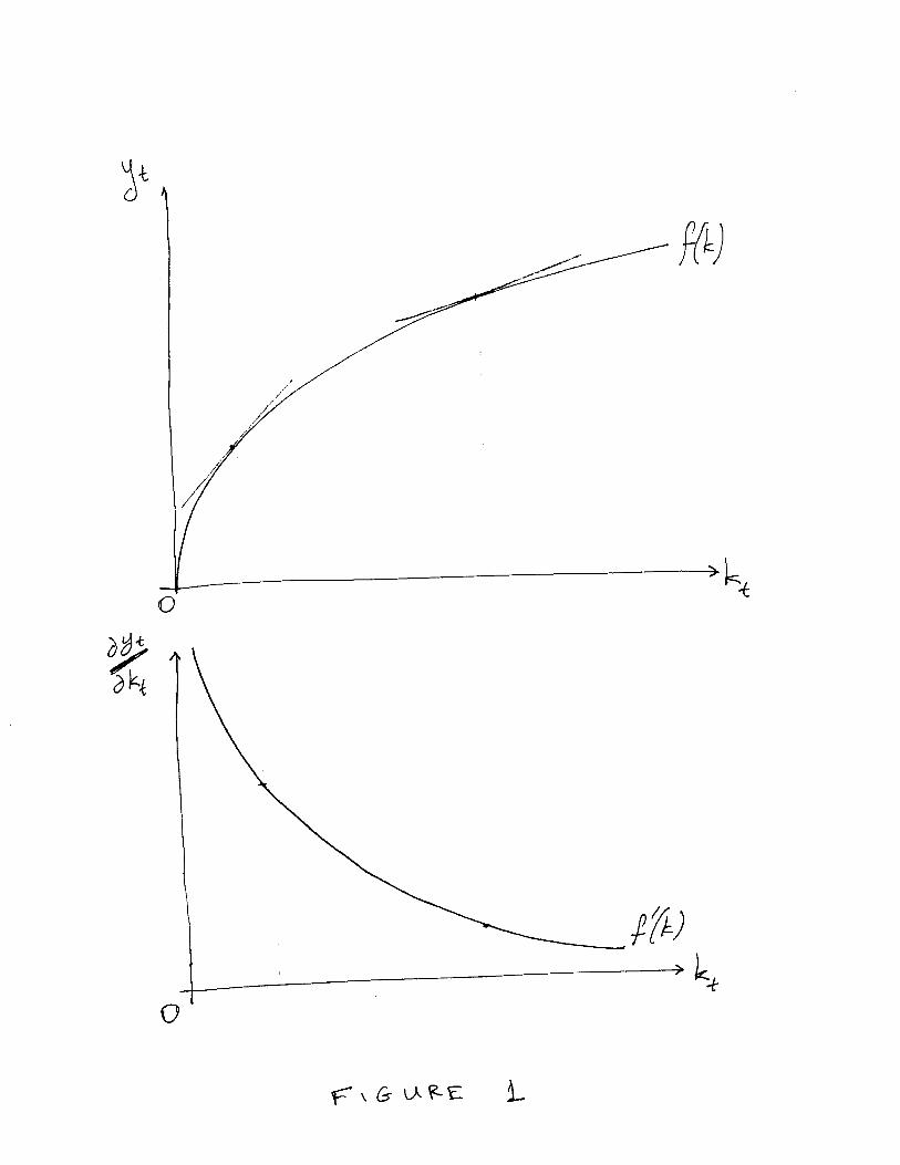
By definition of f and the properties of F,
f(0) = 0,
f 0(k) > 0 > f 00(k)
limk→0
f 0(k) = ∞, limk→∞
f 0(k) = 0
Also,
FK(K,L) = f 0(k)
FL(K,L) = f(k)− f 0(k)k
• The intensive-form production function f and the marginal product of capital f 0 are
illustrated in Figure 1.
• Example: Cobb-Douglas technology
F (K,L) = KαL1−α
In this case,
εK = α, εL = 1− α
and
f(k) = kα.
12
Lecture Notes
2.1.3 The Resource Constraint, and the Law of Motions for Cap-
ital and Labor
• Remember that there is a single good, which can be either consumed or invested. Of
course, the sum of aggregate consumption and aggregate investment can not exceed
aggregate output. That is, the social planner faces the following resource constraint:
Ct + It ≤ Yt (2.3)
Equivalently, in per-capita terms:
ct + it ≤ yt (2.4)
• Suppose that population growth is n ≥ 0 per period. The size of the labor force then
evolves over time as follows:
Lt = (1 + n)Lt−1 = (1 + n)tL0 (2.5)
We normalize L0 = 1.
• Suppose that existing capital depreciates over time at a fixed rate δ ∈ [0, 1]. The
capital stock in the beginning of next period is given by the non-depreciated part of
current-period capital, plus contemporaneous investment. That is, the law of motion
for capital is
Kt+1 = (1− δ)Kt + It. (2.6)
Equivalently, in per-capita terms:
(1 + n)kt+1 = (1− δ)kt + it
13
George-Marios Angeletos
We can approximately write the above as
kt+1 ≈ (1− δ − n)kt + it (2.7)
The sum δ + n can thus be interpreted as the “effective” depreciation rate of per-
capita capital. (Remark: This approximation becomes arbitrarily good as the economy
converges to its steady state. Also, it would be exact if time was continuous rather
than discrete.)
2.1.4 The Dynamics of Capital and Consumption
• In most of the growth models that we will examine in this class, the key of the analysis
will be to derive a dynamic system that characterizes the evolution of aggregate con-
sumption and capital in the economy; that is, a system of difference equations in Ct
and Kt (or ct and kt). This system is very simple in the case of the Solow model.
• Combining the law of motion for capital (2.6), the resource constraint (2.3), and the
technology (2.1), we derive the difference equation for the capital stock:
Kt+1 −Kt ≤ F (Kt, Lt)− δKt − Ct (2.8)
That is, the change in the capital stock is given by aggregate output, minus capital
depreciation, minus aggregate consumption.
kt+1 − kt ≤ f(kt)− (δ + n)kt − ct.
• Remark. Frequently we write the above constraints with equality rather than inequal-
ity, for, as longs as the planner/equilibrium does not waste resources, these constraints
will indeed hold with equality.
14
Lecture Notes
2.1.5 Feasible and “Optimal” Allocations
Definition 1 A feasible allocation is any sequence {ct, kt}∞t=0 ∈¡R2+¢∞
that satisfies the
resource constraint
kt+1 ≤ f(kt) + (1− δ − n)kt − ct. (2.9)
• The set of feasible allocations represents the "choice set" for the social planner. The
planner then uses some choice rule to select one of the many feasible allocations. Later,
we will have to social planner choose an allocation so as to maximize welfare. Here,
we instead assume that the dictaror follows a simple rule-of-thump.
• In particular, consumption is, by assumption, a fixed fraction (1− s) of output:
Ct = (1− s)Yt (2.10)
• Similarly, in per-capita terms, (2.6), (2.4) and (2.2) give the dynamics of capitalwhereas
consumption is given by
ct = (1− s)f(kt).
• From this point and on, we will analyze the dynamics of the economy in per capita
terms only. Translating the results to aggregate terms is a straightforward exercise.
Definition 2 An “optimal” centralized allocation is any feasible allocation that satisfies the
resource constraint with equality and
ct = (1− s)f(kt). (2.11)
• Remark. In the Ramsey model, the optimal allocation will maximize social welfare.
Here, the “optimal” allocation satisfies the presumed rule-of-thump for the planner.
15
George-Marios Angeletos
2.1.6 The Policy Rule
• Combining (2.9) and (2.11), we derive the fundamental equation of the Solow model :
kt+1 − kt = sf(kt)− (δ + n)kt (2.12)
Note that the above defines kt+1 as a function of kt :
Proposition 3 Given any initial point k0 > 0, the dynamics of the dictatorial economy are
given by the path {kt}∞t=0 such that
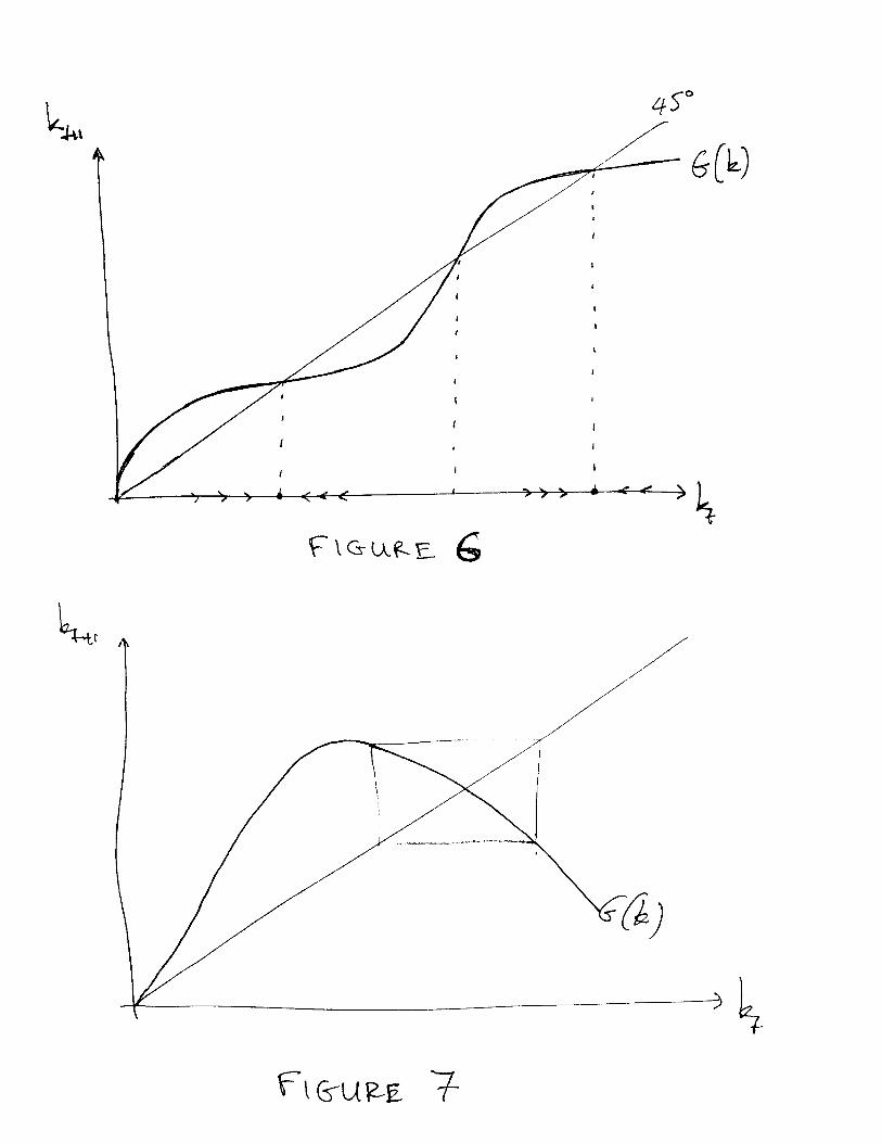
kt+1 = G(kt), (2.13)
for all t ≥ 0, where
G(k) ≡ sf(k) + (1− δ − n)k.
Equivalently, the growth rate of capital is given by
γt ≡kt+1 − kt
kt= γ(kt), (2.14)
where
γ(k) ≡ sφ(k)− (δ + n), φ(k) ≡ f(k)/k.
• Proof. (2.13) follows from (2.12) and rearranging gives (2.14). ¥
• G corresponds to what we will call the policy rule in the Ramsey model. The dynamic
evolution of the economy is concisely represented by the path {kt}∞t=0 that satisfies
(2.12), or equivalently (2.13), for all t ≥ 0, with k0 historically given.
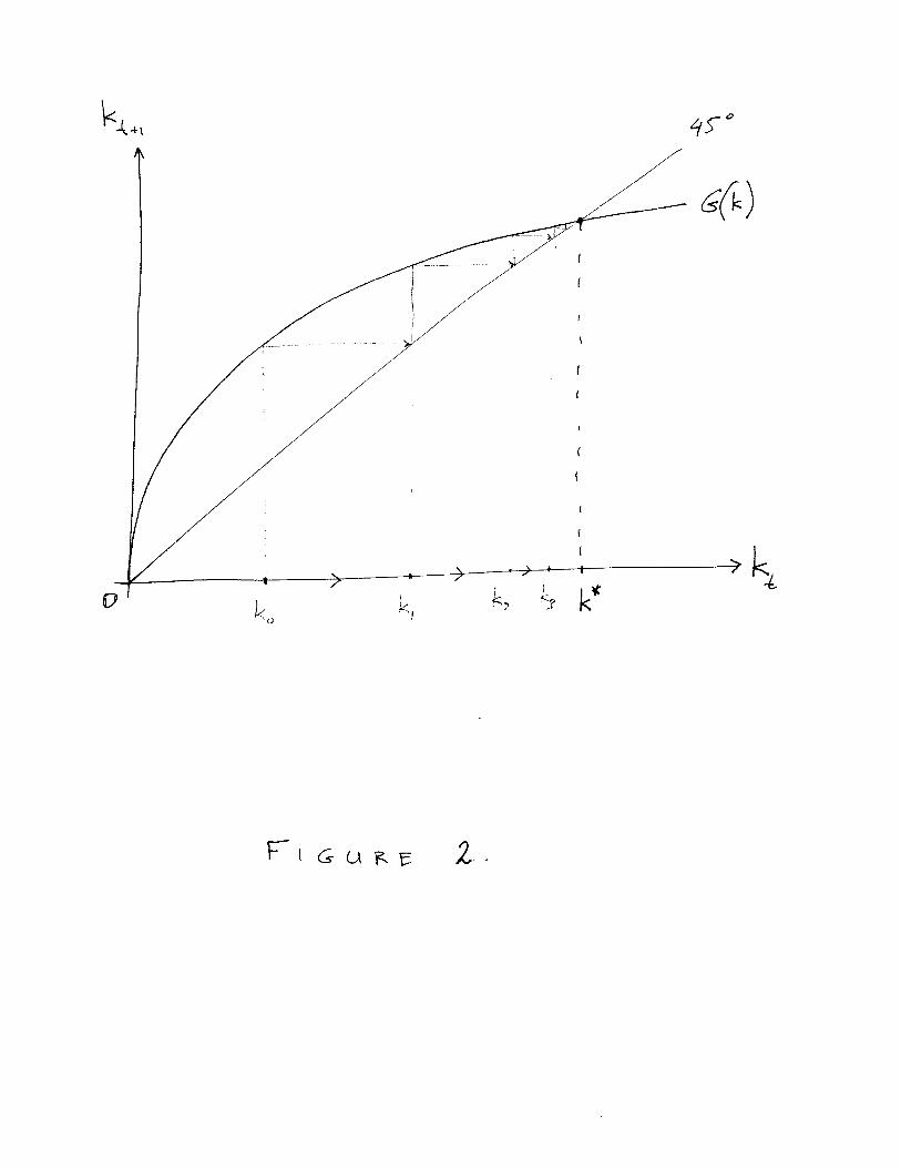
• The graph of G is illustrated in Figure 2.
16
Lecture Notes
• Remark. Think of G more generally as a function that tells you what is the state of the
economy tomorrow as a function of the state today. Here and in the simple Ramsey
model, the state is simply kt. When we introduce productivity shocks, the state is
(kt, At).When we introduce multiple types of capital, the state is the vector of capital
stocks. And with incomplete markets, the state is the whole distribution of wealth in
the cross-section of agents.
2.1.7 Steady State
• A steady state of the economy is defined as any level k∗ such that, if the economy starts
with k0 = k∗, then kt = k∗ for all t ≥ 1. That is, a steady state is any fixed point k∗ of
(2.12) or (2.13). Equivalently, a steady state is any fixed point (c∗, k∗) of the system
(2.9)-(2.11).
• A trivial steady state is c = k = 0 : There is no capital, no output, and no consumption.
This would not be a steady state if f(0) > 0. We are interested for steady states at
which capital, output and consumption are all positive and finite. We can easily show:
Proposition 4 Suppose δ+n ∈ (0, 1) and s ∈ (0, 1). A steady state (c∗, k∗) ∈ (0,∞)2 for the
dictatorial economy exists and is unique. k∗ and y∗ increase with s and decrease with δ and
n, whereas c∗ is non-monotonic with s and decreases with δ and n. Finally, y∗/k∗ = (δ+n)/s.
• Proof. k∗ is a steady state if and only if it solves
0 = sf(k∗)− (δ + n)k∗,
Equivalentlyy∗
k∗= φ(k∗) =
δ + n
s(2.15)
17
George-Marios Angeletos
where
φ(k) ≡ f(k)
k.
The function φ gives the output-to-capital ratio in the economy. The properties of
f imply that φ is continuous (and twice differentiable), decreasing, and satisfies the
Inada conditions at k = 0 and k =∞:
φ0(k) =f 0(k)k − f(k)
k2= −FL
k2< 0,
φ(0) = f 0(0) =∞ and φ(∞) = f 0(∞) = 0,
where the latter follow from L’Hospital’s rule. This implies that equation (2.15) has a
solution if and only if δ+n > 0 and s > 0. and the solution unique whenever it exists.
The steady state of the economy is thus unique and is given by
k∗ = φ−1µδ + n
s
¶.
Since φ0 < 0, k∗ is a decreasing function of (δ+n)/s. On the other hand, consumption
is given by
c∗ = (1− s)f(k∗).
It follows that c∗ decreases with δ + n, but s has an ambiguous effect.
2.1.8 Parenthesis: Global and Local Stability
• Discuss the stability properties of a dynamic system: Eigenvalues, cycles, continuous
vs discrete time.
2.1.9 Transitional Dynamics
• The above characterized the (unique) steady state of the economy. Naturally, we are
interested to know whether the economy will converge to the steady state if it starts
18
Lecture Notes
away from it. Another way to ask the same question is whether the economy will
eventually return to the steady state after an exogenous shock perturbs the economy
and moves away from the steady state.
• The following uses the properties of G to establish that, in the Solow model, conver-
gence to the steady is always ensured and is monotonic:
Proposition 5 Given any initial k0 ∈ (0,∞), the dictatorial economy converges asymp-
totically to the steady state. The transition is monotonic. The growth rate is positive and
decreases over time towards zero if k0 < k∗; it is negative and increases over time towards
zero if k0 > k∗.
• Proof. From the properties of f, G0(k) = sf 0(k) + (1 − δ − n) > 0 and G00(k) =
sf 00(k) < 0. That is, G is strictly increasing and strictly concave. Moreover, G(0) = 0,
G0(0) = ∞, G(∞) = ∞, G0(∞) = (1 − δ − n) < 1. By definition of k∗, G(k) = k iff
k = k∗. It follows that G(k) > k for all k < k∗ and G(k) < k for all k > k∗. It follows
that kt < kt+1 < k∗ whenever kt ∈ (0, k∗) and therefore the sequence {kt}∞t=0 is strictly
increasing if k0 < k∗. By monotonicity, kt converges asymptotically to some k ≤ k∗.
By continuity of G, k must satisfy k = G(k), that is k must be a fixed point of G.
But we already proved that G has a unique fixed point, which proves that k = k∗.
A symmetric argument proves that, when k0 > k∗, {kt}∞t=0 is stricttly decreasing and
again converges asymptotically to k∗. Next, consider the growth rate of the capital
stock. This is given by
γt ≡kt+1 − kt
kt= sφ(kt)− (δ + n) ≡ γ(kt).
Note that γ(k) = 0 iff k = k∗, γ(k) > 0 iff k < k∗, and γ(k) < 0 iff k > k∗. Moreover,
by diminishing returns, γ0(k) = sφ0(k) < 0. It follows that γ(kt) < γ(kt+1) < γ(k∗) = 0
19
George-Marios Angeletos
whenever kt ∈ (0, k∗) and γ(kt) > γ(kt+1) > γ(k∗) = 0 whenever kt ∈ (k∗,∞). This
proves that γt is positive and decreases towards zero if k0 < k∗ and it is negative and
increases towards zero if k0 > k∗. ¥
• Figure 2 depicts G(k), the relation between kt and kt+1. The intersection of the graph
of G with the 45o line gives the steady-state capital stock k∗. The arrows represent the
path {kt}∞t= for a particular initial k0.
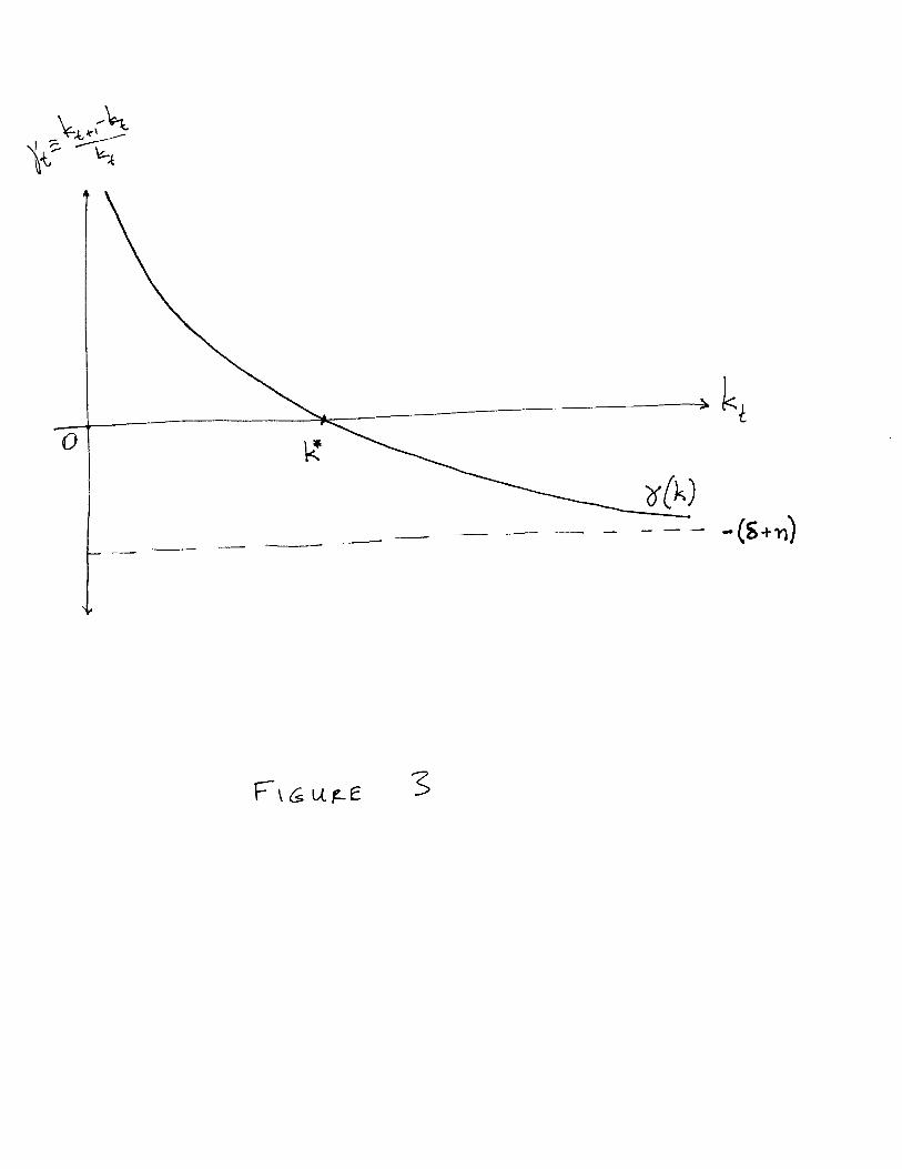
• Figure 3 depicts γ(k), the relation between kt and γt. The intersection of the graph of
γ with the 45o line gives the steady-state capital stock k∗. The negative slope reflects
what we call “conditional convergence.”
• Discuss local versus global stability: Because φ0(k∗) < 0, the system is locally sta-
ble. Because φ is globally decreasing, the system is globally stable and transition is
monotonic.
2.2 Decentralized Market Allocations
• In the previous section, we characterized the centralized allocations dictated by a social
planner. We now characterize the allocations
2.2.1 Households
• Households are dynasties, living an infinite amount of time. We index households by
j ∈ [0, 1], having normalized L0 = 1. The number of heads in every household grow at
constant rate n ≥ 0. Therefore, the size of the population in period t is Lt = (1 + n)t
and the number of persons in each household in period t is also Lt.
20
Lecture Notes
• We write cjt , kjt , bjt , ijt for the per-head variables for household j.
• Each person in a household is endowed with one unit of labor in every period, which
he supplies inelasticly in a competitive labor market for the contemporaneous wage wt.
Household j is also endowed with initial capital kj0. Capital in household j accumulates
according to
(1 + n)kjt+1 = (1− δ)kjt + it,
which we approximate by
kjt+1 = (1− δ − n)kjt + it. (2.16)
Households rent the capital they own to firms in a competitive rental market for a
(gross) rental rate rt.
• The household may also hold stocks of some firms in the economy. Let πjt be the
dividends (firm profits) that household j receive in period t. As it will become clear
later on, it is without any loss of generality to assume that there is no trade of stocks.
(This is because the value of firms stocks will be zero in equilibrium and thus the value
of any stock transactions will be also zero.) We thus assume that household j holds a
fixed fraction αj of the aggregate index of stocks in the economy, so that πjt = αjΠt,
where Πt are aggregate profits. Of course,Rαjdj = 1.
• The household uses its income to finance either consumption or investment in new
capital:
cjt + ijt = yjt .
Total per-head income for household j in period t is simply
yjt = wt + rtkjt + πjt . (2.17)
21
George-Marios Angeletos
Combining, we can write the budget constraint of household j in period t as
cjt + ijt = wt + rtkjt + πjt (2.18)
• Finally, the consumption and investment behavior of household is a simplistic linear
rule. They save fraction s and consume the rest:
cjt = (1− s)yjt and ijt = syit. (2.19)
2.2.2 Firms
• There is an arbitrary number Mt of firms in period t, indexed by m ∈ [0,Mt]. Firms
employ labor and rent capital in competitive labor and capital markets, have access
to the same neoclassical technology, and produce a homogeneous good that they sell
competitively to the households in the economy.
• Let Kmt and L
mt denote the amount of capital and labor that firm m employs in period
t. Then, the profits of that firm in period t are given by
Πmt = F (Km
t , Lmt )− rtK
mt − wtL
mt .
• The firms seek to maximize profits. The FOCs for an interior solution require
FK(Kmt , L
mt ) = rt. (2.20)
FL(Kmt , L
mt ) = wt. (2.21)
• Remember that the marginal products are homogenous of degree zero; that is, they
depend only on the capital-labor ratio. In particular, FK is a decreasing function of
Kmt /L
mt and FL is an increasing function of Km
t /Lmt . Each of the above conditions thus
22
Lecture Notes
pins down a unique capital-labor ratio Kmt /L
mt . For an interior solution to the firms’
problem to exist, it must be that rt and wt are consistent, that is, they imply the same
Kmt /L
mt . This is the case if and only if there is some Xt ∈ (0,∞) such that
rt = f 0(Xt) (2.22)
wt = f(Xt)− f 0(Xt)Xt (2.23)
where f(k) ≡ F (k, 1); this follows from the properties FK(K,L) = f 0(K/L) and
FL(K,L) = f(K/L)− f 0(K/L) · (K/L), which we established earlier.
• If (2.22) and (2.23) are satisfied, the FOCs reduce to Kmt /L
mt = Xt, or
Kmt = XtL
mt . (2.24)
That is, the FOCs pin down the capital labor ratio for each firm (Kmt /L
mt ), but not the
size of the firm (Lmt ). Moreover, because all firms have access to the same technology,
they use exactly the same capital-labor ratio.
• Besides, (2.22) and (2.23) imply
rtXt + wt = f(Xt). (2.25)
It follows that
rtKmt + wtL
mt = (rtXt + wt)L
mt = f(Xt)L
mt = F (Km
t , Lmt ),
and therefore
Πmt = Lm
t [f(Xt)− rtXt − wt] = 0. (2.26)
That is, when (2.22) and (2.23) are satisfied, the maximal profits that any firm makes
are exactly zero, and these profits are attained for any firm size as long as the capital-
labor ratio is optimal. If instead (2.22) and (2.23) were violated, then either rtXt+wt <
23
George-Marios Angeletos
f(Xt), in which case the firm could make infinite profits, or rtXt+wt > f(Xt), in which
case operating a firm of any positive size would generate strictly negative profits.
2.2.3 Market Clearing
• The capital market clears if and only ifZ Mt
0
Kmt dm =
Z 1
0
(1 + n)tkjtdj
Equivalently, Z Mt
0
Kmt dm = Kt (2.27)
where Kt ≡R Lt0
kjtdj is the aggregate capital stock in the economy.
• The labor market, on the other hand, clears if and only ifZ Mt
0
Lmt dm =
Z 1
0
(1 + n)tdj
Equivalently, Z Mt
0
Lmt dm = Lt (2.28)
where Lt is the size of the labor force in the economy.
2.2.4 General Equilibrium: Definition
• The definition of a general equilibrium is more meaningful when households optimize
their behavior (maximize utility) rather than being automata (mechanically save a
constant fraction of income). Nonetheless, it is always important to have clear in mind
what is the definition of equilibrium in any model. For the decentralized version of the
Solow model, we let:
24
Lecture Notes
Definition 6 An equilibrium of the economy is an allocation {(kjt , cjt , ijt)j∈[0,1], (Kmt , L
mt )m∈[0,Mt]}∞t=0,
a distribution of profits {(πjt)j∈[0,1]}, and a price path {rt, wt}∞t=0 such that
(i) Given {rt, wt}∞t=0 and {πjt}∞t=0, the path {kjt , cjt , ijt} is consistent with the behavior of
household j, for every j.
(ii) (Kmt , L
mt ) maximizes firm profits, for every m and t.
(iii) The capital and labor markets clear in every period
2.2.5 General Equilibrium: Existence, Uniqueness, and Charac-
terization
• In the next, we characterize the decentralized equilibrium allocations:
Proposition 7 For any initial positions (kj0)j∈[0,1], an equilibrium exists. The allocation of
production across firms is indeterminate, but the equilibrium is unique as regards aggregate
and household allocations. The capital-labor ratio in the economy is given by {kt}∞t=0 such
that
kt+1 = G(kt) (2.29)
for all t ≥ 0 and k0 =Rkj0dj historically given, where G(k) ≡ sf(k)+(1−δ−n)k. Equilibrium
growth is given by
γt ≡kt+1 − kt
kt= γ(kt), (2.30)
where γ(k) ≡ sφ(k)− (δ + n), φ(k) ≡ f(k)/k. Finally, equilibrium prices are given by
rt = r(kt) ≡ f 0(kt), (2.31)
wt = w(kt) ≡ f(kt)− f 0(kt)kt, (2.32)
where r0(k) < 0 < w0(k).
25
George-Marios Angeletos
• Proof. We first characterize the equilibrium, assuming it exists.
Using Kmt = XtL
mt by (2.24), we can write the aggregate demand for capital asZ Mt
0
Kmt dm = Xt
Z Mt
0
Lmt dm
From the labor market clearing condition (2.28),Z Mt
0
Lmt dm = Lt.
Combining, we infer Z Mt
0
Kmt dm = XtLt,
and substituting in the capital market clearing condition (2.27), we conclude
XtLt = Kt,
where Kt ≡R Lt0
kjtdj denotes the aggregate capital stock. Equivalently, letting kt ≡
Kt/Lt denote the capital-labor ratio in the economy, we have
Xt = kt. (2.33)
That is, all firms use the same capital-labor ratio as the aggregate of the economy.
Substituting (2.33) into (2.22) and (2.23) we infer that equilibrium prices are given by
rt = r(kt) ≡ f 0(kt) = FK(kt, 1)
wt = w(kt) ≡ f(kt)− f 0(kt)kt = FL(kt, 1)
Note that r0(k) = f 00(k) = FKK < 0 and w0(k) = −f 00(k)k = FLK > 0. That is, the
interest rate is a decreasing function of the capital-labor ratio and the wage rate is an
increasing function of the capital-labor ratio. The first properties reflects diminishing
returns, the second reflects the complementarity of capital and labor.
26
Lecture Notes
Adding up the budget constraints of the households, we get
Ct + It = rtKt + wtLt +
Zπjtdj,
where Ct ≡Rcjtdj and It ≡
Rijtdj. Aggregate dividends must equal aggregate profits,R
πjtdj =RΠmt dj. By (2.26), profits for each firm are zero. Therefore,
Rπjtdj = 0,
implying
Ct + It = Yt = rtKt + wtLt
Equivalently, in per-capita terms,
ct + it = yt = rtkt + wt.
From (2.25) and (2.33), or equivalently from (2.31) and (2.32),
rtkt + wt = yt = f(kt)
We conclude that the household budgets imply
ct + it = f(kt),
which is simply the resource constraint of the economy.
Adding up the individual capital accumulation rules (2.16), we get the capital accu-
mulation rule for the aggregate of the economy. In per-capita terms,
kt+1 = (1− δ − n)kt + it
Adding up (2.19) across households, we similarly infer
it = syt = sf(kt).
27
George-Marios Angeletos
Combining, we conclude
kt+1 = sf(kt) + (1− δ − n)kt = G(kt),
which is exactly the same as in the centralized allocation.
Finally, existence and uniqueness is now trivial. (2.29) maps any kt ∈ (0,∞) to a
unique kt+1 ∈ (0,∞). Similarly, (2.31) and (2.32) map any kt ∈ (0,∞) to unique
rt, wt ∈ (0,∞). Therefore, given any initial k0 =Rkj0dj, there exist unique paths
{kt}∞t=0 and {rt, wt}∞t=0. Given {rt, wt}∞t=0, the allocation {kjt , cjt , ijt} for any household
j is then uniquely determined by (2.16), (2.17), and (2.19). Finally, any allocation
(Kmt , L
mt )m∈[0,Mt] of production across firms in period t is consistent with equilibrium
as long as Kmt = ktL
mt . ¥
• An immediate implication is that the decentralized market economy and the centralized
dictatorial economy are isomorphic. This follows directly from the fact that G is the
same under both regimes, provided of course that (s, δ, n, f) are the same:
Corollary 8 The aggregate and per-capita allocations in the competitive market economy
coincide with those in the dictatorial economy.
• Given this isomorphism, we can immediately translate the steady state and the tran-
sitional dynamics of the centralized plan to the steady state and the transitional dy-
namics of the decentralized market allocations:
Corollary 9 Suppose δ + n ∈ (0, 1) and s ∈ (0, 1). A steady state (c∗, k∗) ∈ (0,∞)2 for the
competitive economy exists and is unique, and coincides with that of the social planner. k∗
and y∗ increase with s and decrease with δ and n, whereas c∗ is non-monotonic with s and
decreases with δ and n. Finally, y∗/k∗ = (δ + n)/s.
28
Lecture Notes
Corollary 10 Given any initial k0 ∈ (0,∞), the competitive economy converges asymp-
totically to the steady state. The transition is monotonic. The equilibrium growth rate is
positive and decreases over time towards zero if k0 < k∗; it is negative and increases over
time towards zero if k0 > k∗.
• The above is just a prelude to the first and second welfare theorems, which we will
have once we endow the households with preferences (a utility function) on the basis
of which they will be choosing allocations. In the neoclassical growth model, Pareto
optimal (or efficient) and comptetive equilibrium allocations coincide.
2.3 Shocks and Policies
• The Solow model can be interpreted also as a primitive Real Business Cycle (RBC)
model. We can use the model to predict the response of the economy to productivity
or taste shocks, or to shocks in government policies.
2.3.1 Productivity (or Taste) Shocks
• Suppose output is given by
Yt = AtF (Kt, Lt)
or in intensive form
yt = Atf(kt)
where At denotes total factor productivity.
• Consider a permanent negative shock in productivity. The G(k) and γ(k) functions
shift down, as illustrated in Figure 4. The new steady state is lower. The economy
transits slowly from the old steady state to the new.
29
George-Marios Angeletos
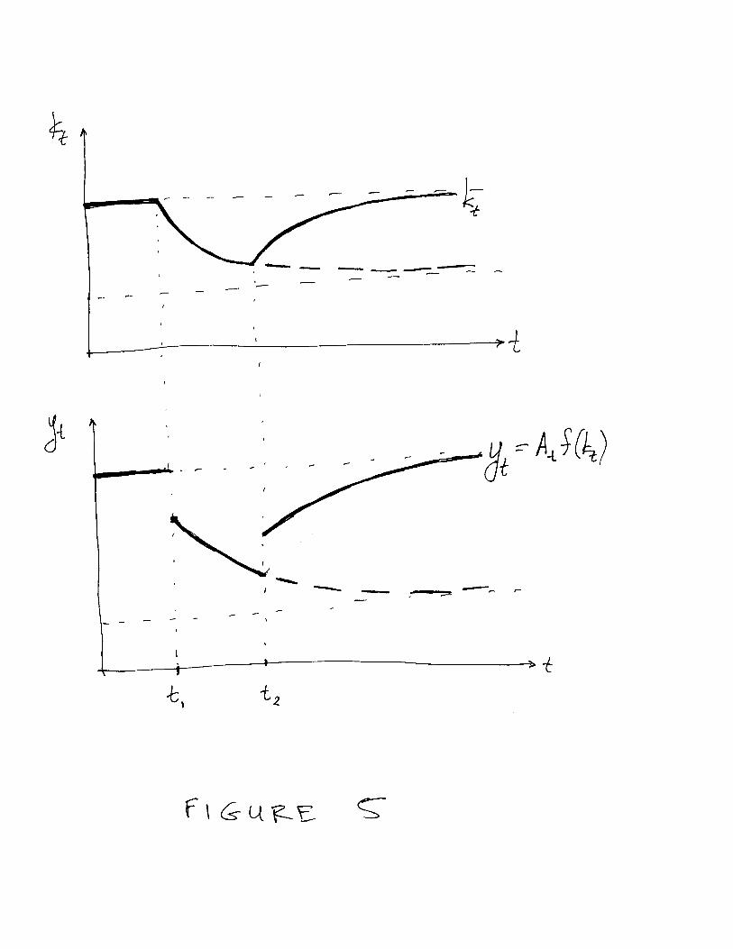
• If instead the shock is transitory, the shift in G(k) and γ(k) is also temporary. Initially,
capital and output fall towards the low steady state. But when productivity reverts
to the initial level, capital and output start to grow back towards the old high steady
state.
• The effect of a prodictivity shock on kt and yt is illustrated in Figure 5. The solid lines
correspond to a transitory shock, whereas the dashed lines correspond to a permanent
shock.
• Taste shocks: Consider a temporary fall in the saving rate s. The γ(k) function shifts
down for a while, and then return to its initial position. What are the transitional
dynamics? What if instead the fall in s is permanent?
2.3.2 Unproductive Government Spending
• Let us now introduce a government in the competitive market economy. The govern-
ment spends resources without contributing to production or capital accumulation.
• The resource constraint of the economy now becomes
ct + gt + it = yt = f(kt),
where gt denotes government consumption. It follows that the dynamics of capital are
given by
kt+1 − kt = f(kt)− (δ + n)kt − ct − gt
• Government spending is financed with proportional income taxation, at rate τ ≥ 0.
The government thus absorbs a fraction τ of aggregate output:
gt = τyt.
30
Lecture Notes
• Disposable income for the representative household is (1−τ)yt.We continue to assume
that consumption and investment absorb fractions 1− s and s of disposable income:
ct = (1− s)(yt − gt),
it = (1− s)(yt − gt).
• Combining the above, we conclude that the dynamics of capital are now given by
γt =kt+1 − kt
kt= s(1− τ)φ(kt)− (δ + n).
where φ(k) ≡ f(k)/k. Given s and kt, the growth rate γt decreases with τ .
• A steady state exists for any τ ∈ [0, 1) and is given by
k∗ = φ−1µ
δ + n
s(1− τ)
¶.
Given s, k∗ decreases with τ .
• Policy Shocks: Consider a temporary shock in government consumption. What are the
transitional dynamics?
2.3.3 Productive Government Spending
• Suppose now that production is given by
yt = f(kt, gt) = kαt gβt ,
where α > 0, β > 0, and α+ β < 1. Government spending can thus be interpreted as
infrastructure or other productive services. The resource constraint is
ct + gt + it = yt = f(kt, gt).
31
George-Marios Angeletos
• We assume again that government spending is financed with proportional income tax-
ation at rate τ , and that private consumption and investment are fractions 1− s and
s of disposable household income:
gt = τyt.
ct = (1− s)(yt − gt)
it = s(yt − gt)
• Substituting gt = τyt into yt = kαt gβt and solving for yt, we infer
yt = kα1−βt τ
β1−β ≡ kat τ
b
where a ≡ α/(1−β) and b ≡ β/(1−β). Note that a > α, reflecting the complementarity
between government spending and capital.
• We conclude that the growth rate is given by
γt =kt+1 − kt
kt= s(1− τ)τ bka−1t − (δ + n).
The steady state is
k∗ =
µs(1− τ)τ b
δ + n
¶1/(1−a).
• Consider the rate τ that maximizes either k∗, or γt for any given kt. This is given by
d
dτ[(1− τ)τ b] = 0⇔
bτ b−1 − (1 + b)τ b = 0⇔
τ = b/(1 + b) = β.
That is, the growth-maximizing τ equals the elasticity of production with respect to
government services. The more productive government services are, the higher their
“optimal” provision.
32
Lecture Notes
2.4 Continuous Time and Conditional Convergence
2.4.1 The Solow Model in Continuous Time
• Recall that the basic growth equation in the discrete-time Solow model is
kt+1 − ktkt
= γ(kt) ≡ sφ(kt)− (δ + n).
We would expect a similar condition to hold under continuous time. We verify this
below.
• The resource constraint of the economy is
C + I = Y = F (K,L).
In per-capita terms,
c+ i = y = f(k).
• Population growth is now given byL
L= n
and the law of motion for aggregate capital is
K = I − δK
• Let k ≡ K/L. Then,k
k=
K
K− L
L.
Substituting from the above, we infer
k = i− (δ + n)k.
33
George-Marios Angeletos
Combining this with
i = sy = sf(k),
we conclude
k = sf(k)− (δ + n)k.
• Equivalently, the growth rate of the economy is given by
k
k= γ(k) ≡ sφ(k)− (δ + n). (2.34)
The function γ(k) thus gives the growth rate of the economy in the Solow model,
whether time is discrete or continuous.
2.4.2 Log-linearization and the Convergence Rate
• Define z ≡ ln k − ln k∗. We can rewrite the growth equation (2.34) as
z = Γ(z),
where
Γ(z) ≡ γ(k∗ez) ≡ sφ(k∗ez)− (δ + n)
Note that Γ(z) is defined for all z ∈ R. By definition of k∗, Γ(0) = sφ(k∗)− (δ + n) =
0. Similarly, Γ(z) > 0 for all z < 0 and Γ(z) < 0 for all z > 0. Finally, Γ0(z) =
sφ0(k∗ez)k∗ez < 0 for all z ∈ R.
• We next (log)linearize z = Γ(z) around z = 0 :
z = Γ(0) + Γ0(0) · z
or equivalently
z = λz
34
Lecture Notes
where we substituted Γ(0) = 0 and let λ ≡ Γ0(0).
• Straightforward algebra gives
Γ0(z) = sφ0(k∗ez)k∗ez < 0
φ0(k) =f 0(k)k − f(k)
k2= −
∙1− f 0(k)k
f(k)
¸f(k)
k2
sf(k∗) = (δ + n)k∗
We infer
Γ0(0) = −(1− εK)(δ + n) < 0
where εK ≡ FKK/F = f 0(k)k/f(k) is the elasticity of production with respect to
capital, evaluated at the steady-state k.
• We conclude thatk
k= λ ln
µk
k∗
¶where
λ = −(1− εK)(δ + n) < 0
The quantity −λ is called the convergence rate.
• In the Cobb-Douglas case, y = kα, the convergence rate is simply
−λ = (1− α)(δ + n),
where α is the income share of capital. Note that as λ → 0 as α → 1. That is,
convergence becomes slower and slower as the income share of capital becomes closer
and closer to 1. Indeed, if it were α = 1, the economy would a balanced growth path.
35
George-Marios Angeletos
• Note that, around the steady state
y
y= εK ·
k
k
andy
y∗= εK ·
k
k∗
It follows thaty
y= λ ln
µy
y∗
¶Thus, −λ is the convergence rate for either capital or output.
• In the example with productive government spending, y = kαgβ = kα/(1−β)τβ/(1−β), we
get
−λ =µ1− α
1− β
¶(δ + n)
The convergence rate thus decreases with β, the productivity of government services.
And λ→ 0 as β → 1− α.
• Calibration: If α = 35%, n = 3% (= 1% population growth+2% exogenous technolog-
ical process), and δ = 5%, then −λ = 6%. This contradicts the data. But if α = 70%,
then −λ = 2.4%, which matches the data.
2.5 Cross-Country Differences and Conditional Con-