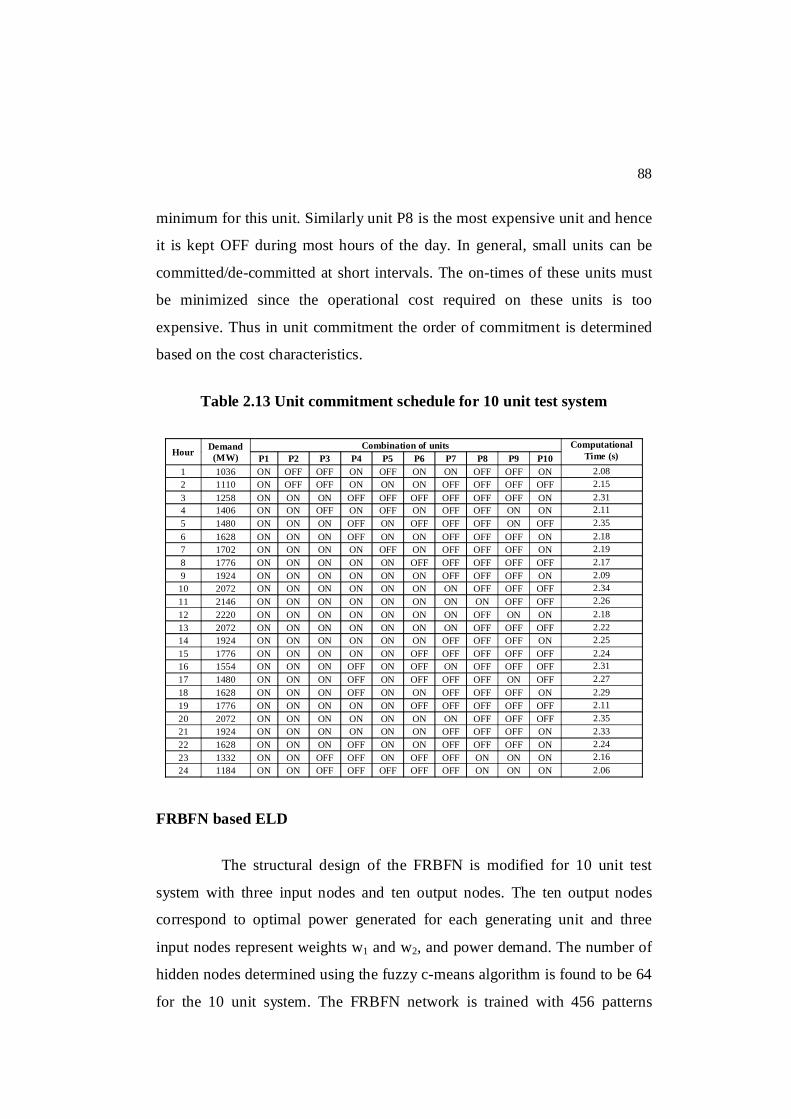
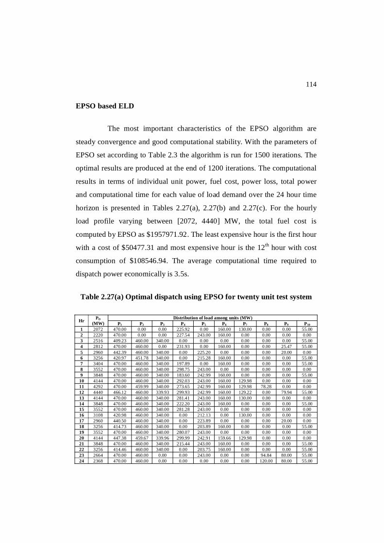
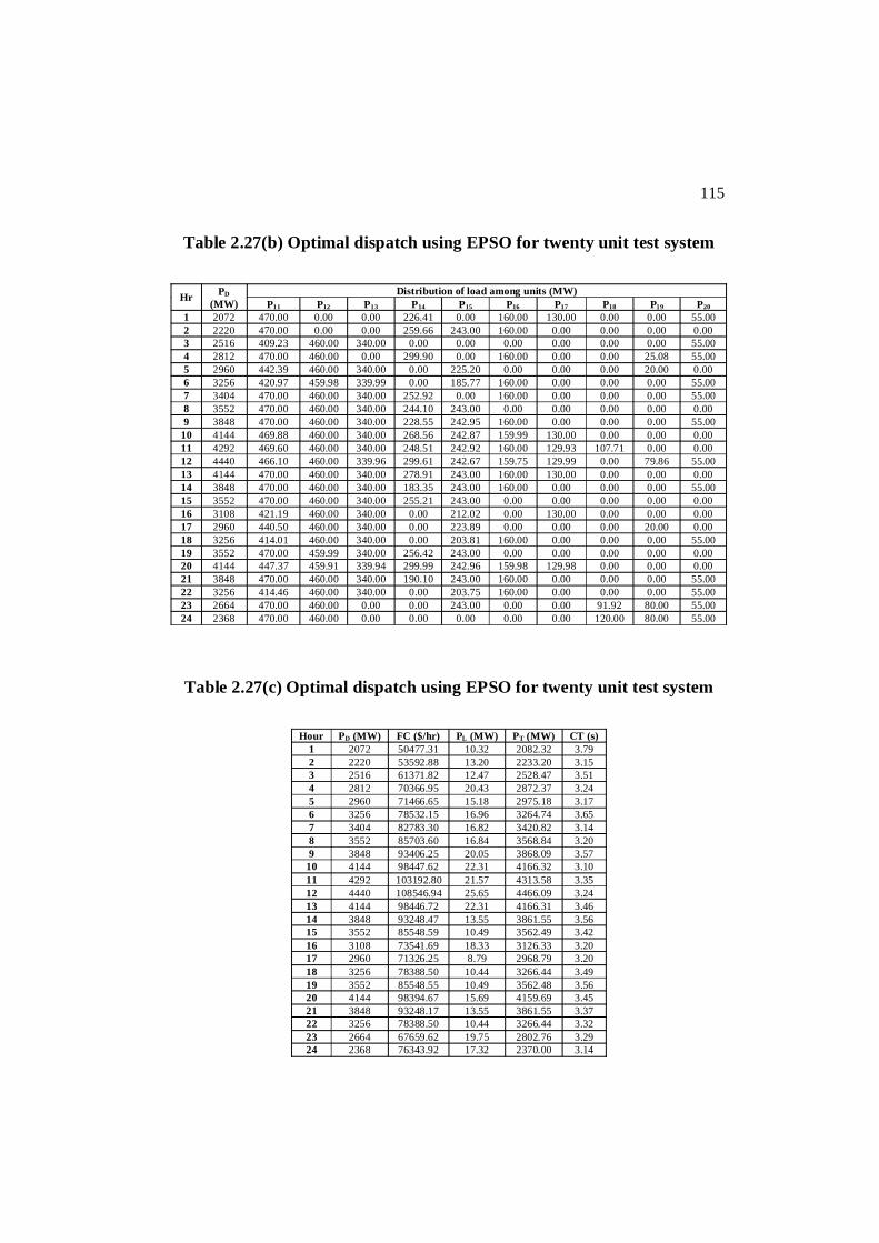
30
CHAPTER 2
UNIT COMMITMENT AND ECONOMIC LOAD
DISPATCH PROBLEM
2.1 INTRODUCTION
The electric power generated is much larger during day time due to
high industrial loads, higher during evenings and early morning due to
residential population usage. Based on the forecasted power requirements for
the successive operating day, the generating units are scheduled on an hourly
basis for the next day’s dispatch, which in turn is forecasted for a week ahead.
The system operators are able to schedule the ON/OFF status and the real
power outputs of the generating units to meet the forecasted demand over a
time horizon. There may exist large variations in the day to day load patterns,
thus enough power has to be generated to meet the maximum load demand. In
addition, it is not economical to run all the units every time. Hence it is
necessary to determine the units of a particular system that are required to
operate for given loads. This problem is known as the unit commitment
(Rajan 2010) problem.
The Economic Load Dispatch (ELD) allocates power to the
committed units thus minimizing the fuel cost. The two major factors to be
considered while dispatching power to generating units are the cost of
generation and the quantity of power supplied. The relation between the cost
of generation and the power levels is approximated by a quadratic
polynomial. To determine the economic distribution of load between the
31
various units in a plant, the quadratic polynomial in terms of the power output
is treated as an optimization problem with cost minimization as the objective
function, considering equality and inequality constraints.
During the past years, several exact and approximate algorithms
have been applied for solving the UC and ELD problems. The exact solutions
to these problems can be obtained through numerical calculations, but cannot
be applied for large practical real-time systems due to the computational
overheads (Vlachogiannis and Lee 2008). Some of these exact methods for
solving UC and ELD are Lambda Iteration method, dynamic programming,
mixed integer programming, branch and bound, Newton’s method, and
Lagrangian relaxation method. The approximate methods include search
algorithms such as Artificial Neural Networks (ANN), Genetic Algorithms
(GA), Tabu Search (TS), Simulated Annealing (SA), Evolutionary
Programming (EP), Particle Swarm Optimization (PSO), Ant colony
optimization (ACO), Artificial Bee Colony (ABC), Differential Evolution
(DE), Bacterial Foraging Algorithm (BFA), Intelligent Waterdrop (IWD) and
Bio-geography based optimization (BBO) algorithms.
During 2002, a fast solution technique for large scale Unit
Commitment Problem using Genetic Algorithm is presented by Senjyu et al
(2002). To reduce search space, unit integration technique is used and an
intelligent mutation is performed using local hill-climbing optimization
technique. A Genetic Algorithm Solution to the Unit Commitment Problem
Based on Real-Coded Chromosomes and Fuzzy Optimization is implemented
by Alma Ademovic et al in the year 2010. They have reported that the fuzzy
optimization had an impact on guiding the GA search and therefore assured
finding a better fuel cost.
Su and Lin (2000) presented a new Hopfield model based approach
for the economic dispatch problem, by including the computational
32
procedures with a series of weighting factor adjustments associated with the
transmission line losses, updating the unit generations and power losses in
order to minimize the value of the energy function. Aravindhababu and Nayar
(2001) presented an on-line approach for solving the ELD using Radial Basis
Function Network (RBFN) which directly produced the optimal lambda
value. This value is applied further to compute the economic generations
iteratively. Huang and Wang (2007) proposed a novel technique that
combines orthogonal least-squares (OLS) and particle swarm optimization
(PSO) algorithms to construct the radial basis function (RBF) network for
real-time power dispatch. In this report, a fuzzy based RBFN is proposed to
solve the unit committed ELD problem. Fuzzy c-means clustering is adopted
as a pre-processing algorithm to the RBFN in order to dimensionally reduce
the data allowing a simpler RBF model for solving ELD problems.
A Particle Swarm Optimization approach to solve the economic
dispatch considering the generator constraints is presented by Gaing (2003).
Many nonlinear characteristics of the generator, such as ramp rate limits,
prohibited operating zone, and non-smooth cost functions are considered in
their method for practical generator operations. Saber and Venayagamoorthy
(2008), attempted to explore the application of Economic Load Dispatch
using Bacterial Foraging Technique with Particle Swarm Optimization based
evolution. They showed that their technique had better information sharing
and conveying mechanisms than other evolutionary methods including PSO,
Bacterial Foraging (BF) and GA. In this thesis, an Enhanced PSO (EPSO)
algorithm is proposed to dispatch the committed units thus minimizing the
fuel cost and making the application more suitable for practical generating
systems.
Iba and Nomana (2008) developed the classical Differential
Evolution (DE) for solving ELD problems with specialized constraint
33
handling mechanisms. Jiriwibhakorn and Khamsawang (2009) applied DE for
ELD by adding the regenerating population procedure in order to improve
escaping from the local minimum. Yare et al (2009) developed three heuristic
algorithms, namely, the genetic algorithm (GA), differential evolution (DE)
and modified particle swarm optimization (MPSO) to solve Economic
Dispatch (ED) problem for two test systems with 6 and 19 generating units.
These heuristic algorithms are applied in literature to solve the nonconvex ED
problems as a replacement for the classical Lagrange based techniques. Wang
et al (2007) used the concept of the 1/5 success rule of evolutionary strategies
in the original Hybrid DE (HDE) to accelerate the search for the global
optimum in ELD problems. The need for fixed and random scale factors in
HDE is overcome by the work of Chiou (2007), in which a variable scaling
factor is added to HDE thus improving the search for the global solution for
ELD problems. Mariani and Coelho (2006) proposed a hybrid technique that
combined the differential evolution algorithm with the generator of chaos
sequences and sequential quadratic programming technique. Aniruddha and
Chattopadhyay (2010) offered a hybrid combination of DE with BBO to
accelerate the convergence speed and to improve the quality of the ELD
solutions. Balamurugan and Subramaniam (2007) presented a Self-Adaptive
Differential Evolution Based Power Economic Dispatch of Generators with
Valve-Point Effects and Multiple Fuel Options. In this work, Differential
Evolution combined with the concept of opposition based learning is
proposed for solving the ELD problem. The initial population is generated
through the concept of opposition based learning, and the algorithm uses only
one population set throughout the optimization process, thus improving the
rate of convergence. In addition, the DE-OBL is improved to form IDE-OBL
by adding a jumping factor to the generation phase, thus improving the
stability in obtaining optimal solutions.
34
Hemamalini and Sishaj (2010) presented an application of
economic load dispatch using Artificial Bee Colony algorithm. They
employed a fuzzy decision theory to extract the best compromise solution.
Later, Sumpavakup et al (2010) published a solution to the optimal power
flow using Artificial Bee Colony algorithm. In their work, the total fuel cost
obtained through the ABC algorithm is similar to the cost obtained through
GA and PSO. In addition, no importance is given to the control parameters of
ABC algorithm. In this thesis work, the ABC algorithm is used to solve the
ELD with more focus towards the tuning of algorithmic control parameters,
thus producing an optimal solution in terms of minimum fuel cost and less
execution time.
In all the literatures reported, either the Unit Commitment or the
Economic Load Dispatch problem is solved individually. Solving UC-ELD
problems using heuristic techniques generates a complete solution for the real
time power system thereby validating these techniques in terms of optimal
solutions, robustness, computational time, and algorithmic efficiency. The
purpose of this work is to find out the advantages of application of the bio-
inspired techniques to the unit commitment and economic load dispatch
problem. An attempt has been made to find out the minimum cost by using
intelligent algorithms such as Fuzzy based Radial Basis Function Network
(FRBFN) (Surekha and Sumathi July 2011), Enhanced Particle Swarm
Optimization (EPSO), Differential Evolution with Opposition Based Learning
(DE-OBL) (Surekha and Sumathi Jan 2012) (Surekha and Sumathi Feb 2012),
Improved Differential Evolution with Opposition Based Learning (IDE-
OBL), Artificial Bee Colony (ABC) optimization (Surekha et al May 2012)
and Cuckoo Search Optimization (CSO) (Surekha and Sumathi Jan 2012). UC
and ELD represent a time decomposed approach to achieve the objective of
economic operation and hence they are viewed as two different optimization
problems. The UC problem deals with a long time span, typically 24 hours or
35
a week. The ON/OFF timing of the generating units is scheduled to achieve
an overall minimum operating cost. ELD is a problem that deals with shorter
time span, typically starting from seconds to approximately 20 minutes. It
allocates the optimal sharing of generation outputs among synchronized units
to meet the forecasted load.
The cost minimization and the rapid response requirement in real
time power systems, necessitate this two step approach. The objective of both
the approaches is to minimize the fuel cost with less time of operation, thus
meeting the constraints imposed. The units in the system are switched
ON/OFF based on an exhaustive search performed by GA. The ON/OFF
schedule is then optimized using the heuristics such as FRBFN, EPSO,
DE-OBL, IDE-OBL, ABC and CSO to dispatch power thus meeting the load
demand without violating the power balance and capacity constraints.
The proposed algorithm is evaluated in terms of UC schedules,
distribution of load among individual units, total fuel cost, power loss, total
power and computational time. For experiment analysis four test systems are
chosen namely the IEEE 30 bus system (6 unit system), 10 unit test system,
Indian utility 75-bus system (15 unit system) and the 20 unit test system
including transmission losses, power balance and generator capacity
constraints. The outcome of the experimental results is compared in terms of
optimal solution, robustness, computational efficiency and algorithmic efficiency.
The chapter is organized as follows: The mathematical formulation
of the UC and ELD problems along with the framework to solve the UC-ELD
problems are given in Section 2.2. The implementation of the proposed
optimization techniques such as GA, FRBFN, EPSO, DE-OBL, IDE-OBL,
ABC and CSO for solving the problem under consideration is delineated in
Section 2.3. Experimental results for the four test systems are explained in
Section 2.4. The comparative analysis based on fuel cost, robustness,
36
computational efficiency and algorithmic efficiency are presented in
Section 2.5 and Section 2.6 summarizes this chapter with future expansions.
2.2 ECONOMIC OPERATION OF POWER GENERATION
Since an engineer is always concerned with the cost of products and
services, the efficient optimum economic operation and planning of electric
power generation have always occupied an important position in the electric
power industry. With large interconnection of the electric networks, the
energy crisis in the world and continuous rise in prices, it is very essential to
reduce the running charges of the electric energy. A saving in the operation of
the system of a small percent represents a significant reduction in operating
cost as well as in the quantities of fuel consumed. The classic problem is the
economic load dispatch of generating systems to achieve minimum operating
cost. In addition, there is a need to expand the limited economic optimization
problem to incorporate constraints on system operation to ensure the security
of the system, thereby preventing the collapse of the system due to unforeseen
conditions. However closely associated with this economic dispatch problem
is the problem of the proper commitment of any array of units to serve the
expected load demands in an ‘optimal’ manner. In this section, the
mathematical formulation of the UC-ELD problem and the proposed
intelligent framework are discussed in detail.
2.2.1 Formulation of UC-ELD Problem
To solve problems related to generator scheduling, numerous trials are
required to identify all the possible solutions, from which the best solution is
chosen. This approach is capable of testing different combinations of units based
on the load requirements (Orero and Irving 1995). At the end of the testing
process the combination with least operating cost is selected as the optimal
schedule. While scheduling generator units, the start up and shut down time are
37
to be determined along with the output power levels at each unit over a specified
time horizon. In turn the start up, shut down and the running cost are maintained
at a minimum. The fuel cost, Fi per unit in any given time interval is a function of
the generator power output as given in Equation (2.1),
n
iiiiii
n
iiiT PcPbaPFF
1
2
1
)( $/Hr (2.1)
where ai, bi, ci represent unit cost coefficients, and Pi denotes the unit power
output. The start-up cost (SC) depends upon the down time of the unit, which
can vary from maximum value, when the unit is started from cold state, to a
much smaller value, if the unit is turned off recently. It can be represented by
an exponential cost curve as shown in Equation (2.2),
)}/exp(1{* ioffiii TSC (2.2)
where i is the hot start up cost, i the cold start up cost, i the unit cooling
time constant and Toff, is the time at which the unit has been turned off.
The total cost TF involved during the scheduling process is a sum
of the running cost, start up cost and shut down cost given by Equation (2.3)
T
t
N
ititititititiT SDUUSCUFCF
1 1,,1,,,. )1( (2.3)
where N is the number of generating units and T is the number of different
load demands for which the commitment has to be estimated. The shut down
cost, SD is usually a constant value for each unit, tiU , is the binary variable
that indicates the ON/OFF status of a unit i in time t. The overall objective is
to minimize FT subject to a number of constraints as follows:
38
i. System hourly power balance is given in Equation (2.4),
where the total power generated must supply the load demand
(PD) and system losses (PL).
LDti
N
iti PPUP ,
1, (2.4)
ii. Hourly spinning reserve requirements (R) must be met.
Spinning reserve is the term used to describe the total amount
of generation available from all the units synchronized on the
system minus the present load plus losses being incurred. This
is mathematically represented using Equation (2.5),
RPPUP LDti
N
iti )(,
1
max, (2.5)
iii. Unit rated minimum and maximum capacities must not be
violated. The power allocated to each unit should be within
their minimum and maximum generating capacity as shown in
Equation (2.6),
max,,
min, tititi PPP (2.6)
iv. The initial states of each generating unit at the start of the
scheduling period must be taken in to account.
v. Minimum up/down (MUT/MDT) time limits of units must not
be violated. This is expressed in Equations (2.7) and (2.8)
respectively.
0)(*)( ,,1,1 itition
it UUMUTT (2.7)
0)(*)( ,1,,1 ititioff
it UUMDTT (2.8)
39
where Toff / Ton is the unit off / on time, while i,tu denotes the unit off / on {0,
1} status.
The principal objective of the economic load dispatch problem is to
find a set of active power delivered by the committed generators to satisfy the
required demand subject to the unit technical limits at the lowest production
cost. The objective of the ELD problem is formulated in terms of the fuel cost
expressed as,
n
iiiiii
n
iiiT PcPbaPFF
1
2
1)(
(2.9)
The total generated power N
iiP
1
should be equal to the sum of total
system demand DP and the transmission loss LP . This power balance equality
constraint is mathematically expressed as,
LD
N
ii PPP
1
(2.10)
where LP is computed using the B coefficients as follows,
00
10
1 1BPBPBPP
N
iii
N
i
N
jjijiL (2.11)
where Bij, B0i and B00 are the transmission loss coefficients obtained from the
B-coefficient matrix. The generator power iP should be limited within the
range stated by the inequality constraint,
maxminiii PPP (2.12)
40
where miniP and max
iP are the minimum and maximum generator limits
corresponding to the ith unit.
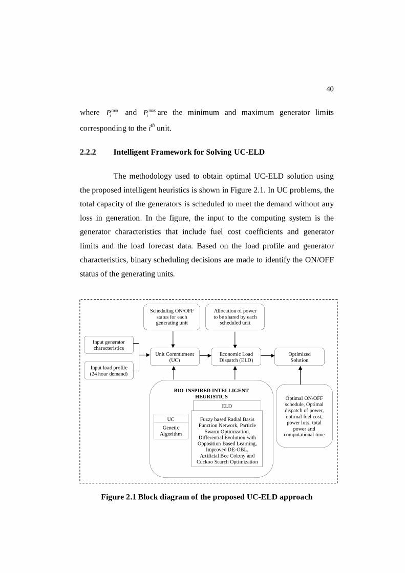
2.2.2 Intelligent Framework for Solving UC-ELD
The methodology used to obtain optimal UC-ELD solution using
the proposed intelligent heuristics is shown in Figure 2.1. In UC problems, the
total capacity of the generators is scheduled to meet the demand without any
loss in generation. In the figure, the input to the computing system is the
generator characteristics that include fuel cost coefficients and generator
limits and the load forecast data. Based on the load profile and generator
characteristics, binary scheduling decisions are made to identify the ON/OFF
status of the generating units.
Figure 2.1 Block diagram of the proposed UC-ELD approach
Input generator characteristics
Input load profile (24 hour demand)
Scheduling ON/OFF status for each generating unit
Allocation of power to be shared by each
scheduled unit
Unit Commitment (UC)
Economic Load Dispatch (ELD)
Optimized Solution
BIO-INSPIRED INTELLIGENT HEURISTICS
UC Genetic
Algorithm
ELD
Fuzzy based Radial Basis Function Network, Particle
Swarm Optimization, Differential Evolution with Opposition Based Learning,
Improved DE-OBL, Artificial Bee Colony and
Cuckoo Search Optimization
Optimal ON/OFF schedule, Optimal dispatch of power, optimal fuel cost, power loss, total
power and computational time
41
The objective of the unit commitment control function is to
minimize the total operational cost to meet the load within the study period of
24 hours ahead by controlling the start up and shut down timing of the
generating units. The scheduled units obtained from the unit commitment
solution using GA correspond to the input data for the economic dispatch
solution. With the commitment known, the economic dispatch problem
allocates the generation economically to the on-line units while satisfying the
demand and system reserve constraints. For each hour, commitment and
de-commitment of generators and the load sharing of each committed unit is
estimated using GA. The Bio-inspired algorithms are utilized to determine the
optimal power dispatch of each unit that is committed to operation at the
specific period, thus minimizing the total generation cost. Optimality of the
UC-ELD problem is analyzed based on fuel cost, power dispatched in
individual units, power loss, and computational time of the algorithms.
2.3 PROPOSED OPTIMIZATION ALGORITHMS
The operation of a modern power system has to incorporate in its
mission a strategy that serves to derive the maximum benefits of an improved
performance and enhanced reliability. The power grid networks have been
analyzed using conventional and enumerative techniques for delivering the
bulk power, reliably and economically, from power plants to the consumers.
Conventional method of solving the generator scheduling problem involves
an exhaustive trial of all the possible solutions and then choosing the best
amongst them is a complex task. For example, in the UC problem the
combination of generating units that produces the least operating cost is taken
as the best schedule as a result of several trial runs. In order to alleviate the
disadvantages associated with conventional strategies in terms of quality
solution, and computational time, bio-inspired intelligent techniques are
explored in this thesis application to solve the UC-ELD problems. The step by
42
step procedure of the algorithms applied to optimize the Unit Commitment
and Economic Load Dispatch problems using the intelligent heuristics are
discussed in detail in this section.
2.3.1 UC Scheduling using Genetic Algorithm
Genetic algorithms are adaptive search techniques based on the
principles and mechanisms of natural selection and “survival of the fittest”
from biological evolution (Goldberg 1989). The algorithm starts with a
population of chromosomes from which a selected group of chromosomes
enter the mating pool. Genetic operators are applied to these chromosomes to
obtain the best solution based on evaluation of the fitness function. The three
prime operators associated with the GA are reproduction, crossover and
mutation. Every generation is made up of a fixed number of solutions
randomly obtained from the solutions of the previous generation. GA may be
phenotypic (operating only on parameters that are placed directly into the
fitness function and evaluated) or genotypic (operating on parameters that are
used to generate behavior in light of external “environmental” factors) (David
Fogel 1995).
In this application, the unit commitment problem is solved using
Genetic Algorithm that generates the on/off status of the generating units. For
the unit commitment problem using GA, a chromosome represents the on/off
status of each unit for a given load demand. For example, if there are six
generating units, the chromosome consists of six genes, each gene represents
the status of one unit. A gene value of 0 represents off status and a gene value
of 1 indicates that the unit is on. The step by step procedure involved in the
implementation of GA for UC problem is explained below:
43
Step 1: Input data
Specify generator cost coefficients, generation power limits for
each unit and transmission loss coefficients (B-matrix) for the test system.
Read hourly load profile of the generators for the test system. Initialize
parameters of GA such as number of chromosomes, population size, number
of generations, selection type, crossover type, mutation type, crossover
probability and mutation probability to suitable values.
Step 2: Initialize GA’s population
Initialize population of the GA randomly, where each gene of the
chromosomes represents commitment of a dispatchable generating unit. The
first step is to encode the commitment space for the UC problem based on the
load curve from the load profile. Units with heavy loads are committed
(binary 1) and units with lighter loads are de-committed (binary 0). The
population consists of a set of UC schedules in the form of a matrix NxT,
where N is the number of generators and T is the time horizon.
Step 3: Computation of total cost
The total generation cost for each chromosome is computed as the
sum of individual unit fuel cost.
Step 4: Computation of cost function and fitness function
The augmented cost function for each chromosomes of population
is computed using,
iiiii
N
ii cPbPaFCF ** 2
1 (2.12)
44
where ai, bi and ci represents unit cost coefficients, and Pi is the unit power
output. The fitness function of chromosomes is calculated as the inverse of
the augmented cost function.
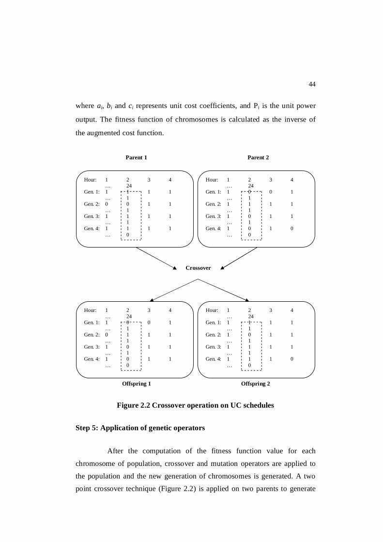
Figure 2.2 Crossover operation on UC schedules
Step 5: Application of genetic operators
After the computation of the fitness function value for each
chromosome of population, crossover and mutation operators are applied to
the population and the new generation of chromosomes is generated. A two
point crossover technique (Figure 2.2) is applied on two parents to generate
Offspring 1 Offspring 2
Parent 2 Parent 1
Hour: 1 2 3 4 … 24 Gen. 1: 1 1 1 1 … 1 Gen. 2: 0 0 1 1 … 1 Gen. 3: 1 1 1 1 … 1 Gen. 4: 1 1 1 1 … 0
Hour: 1 2 3 4 … 24 Gen. 1: 1 0 0 1 … 1 Gen. 2: 1 1 1 1 … 1 Gen. 3: 1 0 1 1 … 1 Gen. 4: 1 0 1 0 … 0
Hour: 1 2 3 4 … 24 Gen. 1: 1 0 0 1 … 1 Gen. 2: 0 1 1 1 … 1 Gen. 3: 1 0 1 1 … 1 Gen. 4: 1 0 1 1 … 0
Hour: 1 2 3 4 … 24 Gen. 1: 1 1 1 1 … 1 Gen. 2: 1 0 1 1 … 1 Gen. 3: 1 1 1 1 … 1 Gen. 4: 1 1 1 0 … 0
Crossover
45
two offspring. The offspring are evaluated for fitness and the best one is
retained while the worst is discarded from the population. The mutation
operation is performed by selecting a chromosome with specified probability.
The chosen chromosome is decoded to its binary equivalent with the unit number and the time period is selected randomly for the flip bit mutation operation.
Step 6: The algorithm terminates after a specified number of generations have
reached. If the termination condition is not satisfied then go to Step 3.
Using the above procedure the generating units of the test systems
are committed/de-committed accordingly and based on these ON/OFF
schedules, the economic dispatch is performed by applying FRBFN, EPSO,
DE-OBL, IDE-OBL, ABC and CSO algorithms.
2.3.2 Fuzzy c-means based Radial Basis Function Network for ELD
The proposed methodology of implementing the RBF network to
solve the ELD problem is shown in Figure 2.3. The training data based on the
selected test systems for different power demands with varying weights are
set by the Lambda Iteration Method (LIM). The values generated should be capable of satisfying all load profiles.
Figure 2.3 Schematic of proposed FRBFN methodology
Clustering technique Generation of Training data
through LI Method
Construction of RBF network
Determine number of centers Normalization of
training data
Formation of new centers using grouping
and averaging
Deduct repetitive centers Real-time economic
dispatch
46
Fuzzy c-means clustering
Application of clustering methods requires the number of known
clusters in advance. There are two options for clustering – validity measures
and compatible clustering. The data samples are clustered several times, each
time with a different number of clusters ],2[ nk in validity measures, while
in the compatible type of clustering, the algorithms starts with a large number
of clusters then proceeding by gradually merging similar clusters to obtain
fewer clusters. (Meng et al 2010). In order to validate the non-linearity of the
system, the value of k should be large enough.
The choice of selecting the number of hidden units in a neural
network is one of the most challenging tasks, requiring more experimentation.
In this thesis, a fuzzy c-means clustering approach is adopted to specify the
range of hidden layer neurons in the RBF network. Consider ix is the
data patterns in the feature space. Let the initial cluster number be 2/nk ,
and test whether a new center should be added based on the performance of
the network. The new cluster center 1kc is added from the remaining
samples ],,,[ 21 kccc . The fuzzy membership matrix is then updated with new
centers and the process is repeated until the condition nk is satisfied. The clustering algorithm is performed by minimizing the objective function,
n
i
k
jji
mjim cxuxcuJ
1 1);,(min (2.13)
where m is a real number greater than 1, uji is the degree of membership
of xi in the cluster j, xi is the ith d-dimensional measured data, cj is the
d-dimension center of the cluster, and ||*|| is the norm expressing the
similarity between measured data and the center.
47
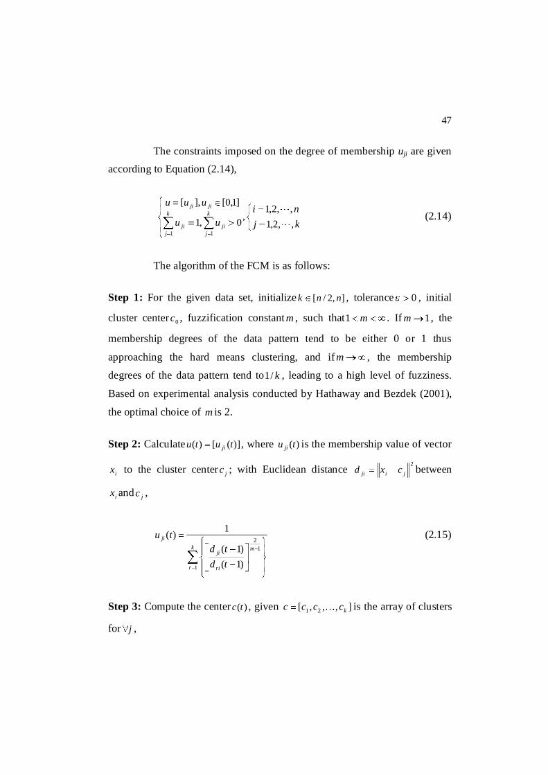
The constraints imposed on the degree of membership uji are given
according to Equation (2.14),
kjni
uu
uuuk
j
k
jjiji
jiji
,,2,1,,2,1
,0,1
]1,0[],[
1 1
(2.14)
The algorithm of the FCM is as follows:
Step 1: For the given data set, initialize ],2/[ nnk , tolerance 0 , initial
cluster center 0c , fuzzification constant m , such that m1 . If 1m , the
membership degrees of the data pattern tend to be either 0 or 1 thus
approaching the hard means clustering, and ifm , the membership
degrees of the data pattern tend to k/1 , leading to a high level of fuzziness.
Based on experimental analysis conducted by Hathaway and Bezdek (2001),
the optimal choice of m is 2.
Step 2: Calculate )]([)( tutu ji , where )(tu ji is the membership value of vector
ix to the cluster center jc ; with Euclidean distance 2
jiji cxd between
ix and jc ,
k
r
m
ri
ji
ji
tdtd
tu
1
12
)1()1(
1)( (2.15)
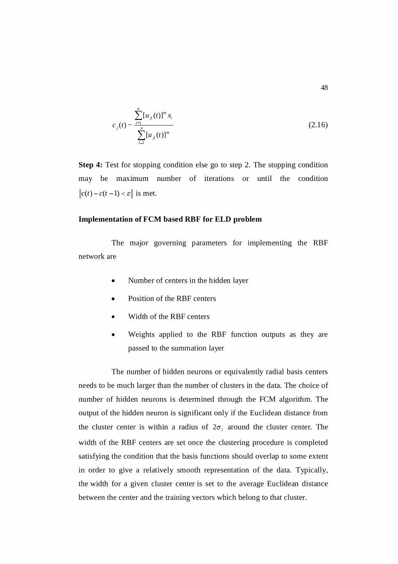
Step 3: Compute the center )(tc , given ],,,[ 21 kcccc is the array of clusters
for j ,
48
m
n
iji
im
n
iji
j
tu
xtutc
])([
])([)(
1
1 (2.16)
Step 4: Test for stopping condition else go to step 2. The stopping condition
may be maximum number of iterations or until the condition
)1()( tctc is met.
Implementation of FCM based RBF for ELD problem
The major governing parameters for implementing the RBF
network are
Number of centers in the hidden layer
Position of the RBF centers
Width of the RBF centers
Weights applied to the RBF function outputs as they are
passed to the summation layer
The number of hidden neurons or equivalently radial basis centers
needs to be much larger than the number of clusters in the data. The choice of
number of hidden neurons is determined through the FCM algorithm. The
output of the hidden neuron is significant only if the Euclidean distance from
the cluster center is within a radius of i2 around the cluster center. The
width of the RBF centers are set once the clustering procedure is completed
satisfying the condition that the basis functions should overlap to some extent
in order to give a relatively smooth representation of the data. Typically,
the width for a given cluster center is set to the average Euclidean distance
between the center and the training vectors which belong to that cluster.
49
The application of RBF network consists of two phases, training
and testing. The accuracy of RBF network model depends on the proper
selection of training data. The inputs of the training network are power
demand, weights w1 and w2, while the outputs constitute the power generated
by the generating units. The step-by-step procedure involved in the
implementation of ELD using FCM based RBF network is elaborated below:
Step 1: Divide the data set into training, and testing sets to evaluate the
proposed network performance.
Step 2: Initialize suitable values for the range of cluster, initial cluster center,
tolerance value for FCM, and number of maximum iterations.
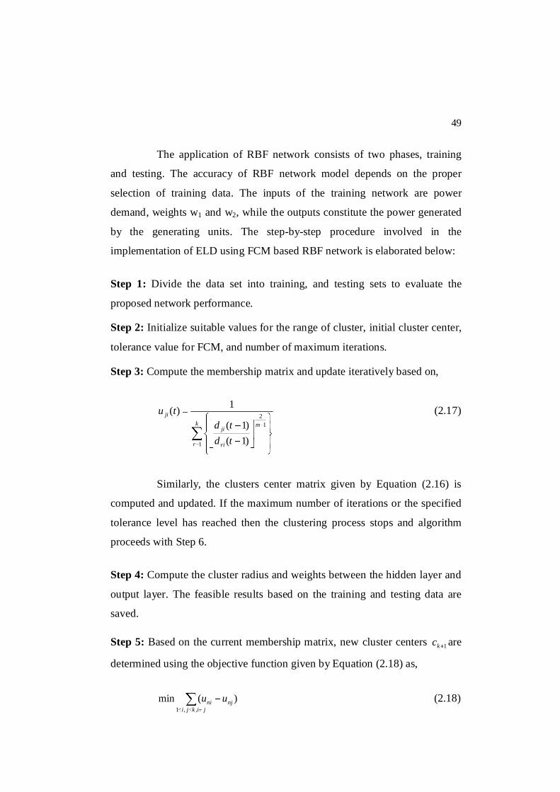
Step 3: Compute the membership matrix and update iteratively based on,
k
r
m
ri
ji
ji
tdtd
tu
1
12
)1()1(
1)( (2.17)
Similarly, the clusters center matrix given by Equation (2.16) is
computed and updated. If the maximum number of iterations or the specified
tolerance level has reached then the clustering process stops and algorithm
proceeds with Step 6.
Step 4: Compute the cluster radius and weights between the hidden layer and
output layer. The feasible results based on the training and testing data are
saved.
Step 5: Based on the current membership matrix, new cluster centers 1kc are
determined using the objective function given by Equation (2.18) as,
jikji
njni uu,,1
)(min (2.18)
50
Go to step 3 to check if the clustering process has completed.
Step 6: The center model that produces minimum error is selected and the
output results are computed based on the testing data.
Figure 2.4 Flow chart of ELD using RBF network
Figure 2.4 shows the steps involved in solving ELD problem using
RBF network. The parameters such as cost coefficients ii ba , and ic , minimum
and maximum power generated in the thi unit, minGiP and maxGiP , are given as
input to the input nodes. Along with the input parameters, the test data of the
inputs are also provided. While propagating along the hidden layers, the
weights are updated and the centers are chosen using random selection
method. The network is trained through the algorithm and the error values are
computed. If the difference between the target and trained data is below the
tolerance value, the algorithm is stopped and the results are displayed,
otherwise the process is repeated until the error converges. The accuracy of
the RBF network also depends upon the proper selection of the training data.
The more uniform the training data are distributed, the faster the network
converges thus providing the optimal solution.
51
2.3.3 Solution to ELD using Enhanced Particle Swarm Optimization
Algorithm
PSO is one of the modern heuristic algorithms suitable to solve
large-scale non-convex optimization problems. It is a population-based search
algorithm and searches in parallel using a group of particles (Yongqiang
Wang et al 2010). In this thesis, Enhanced PSO (EPSO) is applied to solve the
ELD problem. The EPSO is an improved version of the conventional PSO,
being inspired by the study of birds and fish flocking. In EPSO, a constriction
factor is introduced in the velocity update formula to ensure faster
convergence. In PSO algorithm, each particle in the swarm represents a
solution to the problem and is defined with its position and velocity. Each
particle has a position represented by a position-vector xi (i is the index of the
particle), and a velocity represented by a velocity-vector vi. Each particle
remembers its own best position so far in vector xi#, and its jth dimensional
value is xij#. The best position-vector among the swarm so far is then stored in
a vector x , and its jth dimensional value is xj*. During the iteration time t, the
update of the velocity from the previous velocity to the new velocity is
determined by Equation (2.19). The new position is then determined by the
sum of the previous position and the new velocity by Equation (2.20).
))()(())()(()()1( *22
*11 txtxrctxtxrctwvtv ijjijijjiij (2.19)
)1()()1( tvtxtx ijijji (2.20)
where w is the inertia weight factor, r1 and r2 are the random numbers, which
are used to maintain the diversity of the population, and are uniformly
distributed in the interval [0,1] for the jth dimension of the ith particle, c1 is a
positive constant, called as coefficient of the self-recognition component
(cognitive component), c2 is a positive constant, called as coefficient of the
52
social component. From Equation (2.19), a particle decides where to move
next, considering its own experience, which is the memory of its best past
position, and the experience of its most successful particle in the swarm.
In EPSO, the acceleration constants c1, c2 and the inertia weight w
are modified thus in turn affecting the velocity and position update equations.
The constriction factor k is computed using the social and cognitive
components according to,
ccc
k42
22
(2.21)
where c=c1+c2, such that c1+c2
Similarly the inertia weight w of the particle is also updated during
the iterations in a non-linear fashion according to Equation (2.22),
minminmax max_
max_*)( witer
iteriterwww (2.22)
where wmax is the maximum inertia weight, wmin is the minimum inertia
weight, max_iter is the maximum number of iterations run by the EPSO and
iter is the value of the current iteration.
Thus the position and velocity are updated as follows:
))()(())()(()()1( *22
*11 txtxrctxtxrctwkvtv ijjijijjiij (2.23)
)1()()1( tvtxtx ijijji (2.24)
The algorithm for implementing EPSO to solve the ELD problem is
shown below:
53
Step 1: Initialize the PSO parameters such as Population size, Maximum
inertia weight, Minimum inertia weight, Initial velocity, Initial position,
Cognitive factor, Social factor, error gradient and maximum number of
iterations.
Step 2: To each individual of the population Pg (generator power), employ the
B-coefficient loss formula to calculate the transmission loss PL, according to,
00
10
1 1BPBPBPP
N
iGii
N
i
N
jGjijGiL (2.25)
where Bij, B0i and B00 are the transmission loss coefficients obtained from the
B-coefficient matrix.
Step 3: Calculate the fitness value of each individual in the population using
the fitness function given by Equation (2.26),
pbct PF
fcos
1 (2.26)
where Fcost and Ppbc are given by
)(
))((1
minmax
1min
cos FF
FPFabsF
N
iii
t (2.27)
N
iLDipbc PPPP
1
2)(1 (2.28)
where, Fmax is the maximum generation cost among all individuals in the
initial population, Fmin is the minimum generation cost among all individuals
in the initial population, Pi is the power generated by each unit, PD is the
power demand and PL is the power loss.
Step 4: Compare each individual’s evaluation value with its pbest. The best
evaluation value among the pbests is denoted as gbest.
54
Step 5: Modify the member velocity of each individual according to
Equation (2.23).
Step 6: Modify the member position of each individual according to
Equation (2.24).
Step 7: If the evaluation value of each individual is better than the previous
pbest, the current value is set to be pbest. If the best pbest is better than gbest,
the value is set to be gbest.
Step 8: If the number of iterations reaches the maximum, then go to Step 9.
Otherwise, go to Step 3.
Step 9: The individual that generates the latest gbest is the optimal power
generation for each unit. Save the computed results.
The aforementioned steps are followed to estimate an optimized
solution to the UC-ELD problem for all the test systems considered in this thesis.
2.3.4 Improved Differential Evolution with Opposition Based Learning
for ELD
This section presents Differential Evolution algorithm combined
with Opposition Based Learning (DE-OBL) and its improved version IDE-
OBL to solve Economic Load Dispatch problem with non-smooth fuel cost
curves considering transmission losses, power balance and capacity
constraints. The proposed DE-OBL algorithm varies from the Standard
Differential Evolution (SDE) algorithm in terms of three factors such as initial
population, mutation, and population size. The proposed IDE-OBL is
improved over the DE-OBL by adding an opposition based generation
jumping step which selects fitter individuals based on opposite points. The
concept of OBL and the step by step procedure to implement the IDE-OBL
for solving ELD are explained below.
55
Concept of OBL
In general, heuristic optimization methods start with few initial
solutions in a population and try to improve them towards optimal solutions
during generations. The optimization process terminates when some
predefined criteria are satisfied. Without any a priori information about the
solutions to the problem under consideration, the optimization starts with a set
of random presumptions. The chance of obtaining a fitter solution can be
attained through the opposite solution. By monitoring the opposite solution,
the fitter presumed solution can be chosen as an initial solution. In fact,
according to probability theory, 50% of the time the opposite presumption of
the solution is better. Therefore, based on the fitness, two close presumptions
have the potential to accelerate convergence. This approach is not only
applied to initial solutions but also continuously to each solution in the current
population.
Opposition-based population initialization
Consider a point ),,,( 21 nxxxP , with D-dimensional space
consisting of candidate solutions. Let (.)f be the fitness function used to
measure the fitness of the candidate solutions. If
Diqpx iii ,...,2,1],[ represents a real number, then the opposite points of
ix (denoted as ix ) is defined as
iiii xqpx (2.29)
Based on Equation (2.29), ),,,( 21 nxxxP represents the opposite
of ),,,( 21 nxxxP . If )()( PfPf , then P can be replaced with P ,
otherwise the optimization procedure continues with P . Thus the point and its
56
opposite point are evaluated simultaneously in order to continue the
generations with the fitter individuals.
Opposition-based generation jumping
In IDE-OBL, the evolutionary process can be forced to jump to a
new solution candidate, which may be fitter than the current one. Based on a
jumping rate Jr, after generating new population by selection, crossover, and
mutation, the opposite population is calculated and the Np fittest individuals
are selected from the union of the current population and the opposite
population. Unlike opposition-based initialization, the opposite population for
generation jumping is calculated dynamically using the opposite of each
variable. Such dynamic opposition increases the chance to find fitter opposite
points, which helps in fine tuning. By staying within variables’ interval static
boundaries, the evolutionary process would jump outside of the shrunken
solution space and the knowledge of current reduced space (converged
population) would not be utilized (Rahnamayan et al, 2008). Hence, opposite
points are calculated by using the variables’ current interval in the population.
Proposed IDE-OBL for ELD
Though SDE has emerged as one of the most popular technique for
solving optimization problem, it has been observed that the convergence rate
of SDE does not meet the expectations in case of multi-objective problems.
Hence, certain modifications using the concept of opposition based learning
are performed on the SDE. The proposed IDE-OBL varies from the basic
SDE in terms of the following factors:
IDE-OBL uses the concept of opposition based learning in the
initialization phase while SDE uses the uniform random
numbers for initialization of population.
57
During mutation, DE-OBL chooses the best individual among
the three points as the mutant individual whereas in SDE, a
random choice is made with equal choice of any of the three
being selected. In IDE-OBL, an opposition based generation
phase is added with a jumping factor to determine fitter
opposite points.
SDE uses two sets of population – current population and an
advanced population for next generation individuals. Both
DE-OBL and IDE-OBL use only one population set
throughout the optimization process, which is updated in
successive generations with the best individuals found in each
generation.
The steps of the proposed algorithm for implementing ELD are
explained below:
Initialization: The basic step in the IDE-OBL optimization is to create an
initial population of candidate solutions by assigning random values to each
decision parameter of each individual of the population. A population P
consisting of NP individuals is constructed in a random manner such that the
values lie within the feasible bounds minjX and max
jX of the decision variable,
according to the following rule,
DjandNiXXrandXX Pjjjji ,,2,1,,2,1,]1,0[ minmaxmin)0(, (2.30)
where ]1,0[rand represents a uniform random number in the interval [0,1], minjX and max
jX are the lower and upper bounds for the jth component
respectively, D is the number of decision variables. Each individual member
of the population consists of an N-dimensional vector
58
},,,{ 21)0(
Ni PPPX where the ith element of )0(iX represents the power output
of the ith generating unit.
An opposite population addP is constructed using the rule,
jijjji PXXY ,maxmin)0(
, , (2.31)
where jiP , denotes the points of population P . The new population newP for the
proposed approach is formed by combining the best individuals of both
populations P and addP as follows
)0(
,)0(
, jijinew YXP (2.32)
Mutation: Next generation offspring are introduced into the population
through the mutation process. Mutation is performed by choosing three
individuals from the population newP in a random manner. Let raX , rbX and
rcX represent three random individuals such that ircrbra , upon which
mutation is performed during the Gth generation as,
PGrc
Grb
Gbest
Gi NiXXFXV ,2,1,1
(2.33)
where 1GiV is the perturbed mutated individual and G
bestX represents the best
individual among three random individuals. The difference of the remaining
two individuals is scaled by a factor F, which controls the amplification of the
difference between two individuals so as to avoid search stagnation and to
improve convergence.
Crossover: New offspring members are reproduced through the crossover
operation based on binomial distribution. The members of the current
population (target vector) GjiX , and the members of the mutated individual
59
1,GjiV are subject to crossover operation thus producing a trial vector 1
,G
jiU
according to,
otherwiseXCrandifV
U Gji
rGjiG
ji ,]1,0[,
,
1,1
, (2.34)
where rC is the crossover constant that controls the diversity of the population
and prevents the algorithm from getting trapped into the local optima. The
crossover constant must be in the range of [0 1]. 1rC implies the trial vector
will be composed entirely of the mutant vector members and 0rC implies
that the trial vector individuals are composed of the members of parent vector.
Equation (2.34) can also be written as
r1G
ji,rG
ji,1G
ji, CV + )C -(1 X= U (2.35)
Selection: Selection procedure is performed with the trial vector and the
target vector to choose the best set of individuals for the next generation. In
this proposed approach, only one population set is maintained and hence the
best individuals replace the target individuals in the current population. The
objective values of the trial vector and the target vector are evaluated and
compared. For minimization problems like ELD, if the trial vector has better
value, the target vector is replaced with the trial vector as per,
PG
i
Gi
Gi
GiG
i NiforotherwiseX
XfUfifUX ,,2,1;
,)()(, 11
(2.36)
Fitness evaluation: The objective function for the ELD problem based on the
fuel cost and power balance constraints is framed as
N
iLD
N
iii PPPikPFxf
11)()( (2.37)
60
where k is the penalty factor associated with the power balance constraint,
)( ii PF is the ith generator cost function for output power Pi, N is the number of
generating units, DP is the total active power demand and LP represents the
transmission losses. For ELD problems without transmission losses, setting
k=0 is most rational, while for ELD including transmission losses, the value
of k is set to 1.
Generation jumping: The maximum and minimum values of each variable in
current population ]max,[min pj
pj are used to calculate opposite points instead
of using the predefined interval boundaries ],[ maxminjj XX of the variables
according to Equation (2.37a)
DjNiPY pjipj
pjji ,,2,1;,,2,1,maxmin ,
)0(, (2.37a)
The fittest individuals are selected from the new population set ],[ , jii YX as
the current population.
The pseudocode of the proposed approach is shown below:
Generate an initial population P randomly with each individual representing the power output of the ith generating unit according to Equation (2.30).
Generate an additional population addP according to Equation (2.31)
Obtain the new population newP as per Equation (2.32)
Evaluate fitness for each individual in newP based on Equation (2.37)
While termination criteria not satisfied For i = 1 to NP
Mutate random members in newP to obtain 1GiV
Perform crossover on GiX and 1
,G
jiU
Evaluate fitness function of GiX and 1G
iU
If )()( 1 Gi
Gi XfUf
61
Replace existing population with 1GiU
End if End for Obtain opposite population for generation jumping (Equation (2.37a))
Select the fittest individuals from the set ],[ , jii YX as the current population
End While
2.3.5 ELD using Artificial Bee Colony Optimization
The Artificial Bee Colony (ABC) optimization algorithm developed
by Karaboga and Basturk (2007) is becoming more popular recently, due to
the foraging behavior of honeybees. ABC is a population based search
technique, in which the individuals known as the food positions are modified
by the artificial bees during course of time. The objective of the bees in turn is
to discover the food sources with high nectar concentration. The colony of
artificial bees is grouped into employed bees, onlooker bees and scout bees.
During initialization phase, the objective of the problem is defined along with
the ABC algorithmic control parameters. An employed bee is assigned for
every food source available in the problem. In employed bee phase, the
employed bee stays on a food source and provides the neighborhood of the
source in its memory. During the onlooker phase, onlooker bees watch the
waggle dance of employed bees within the hive to choose a food source. The
employed bee whose food source has been abandoned becomes the scout bee.
Scout bees search for food sources randomly during the scout phase. Thus the
local search is carried out by the employed bees and the onlooker bees while
the global search is performed by the onlooker and the scout bees, thus
maintaining a balance between the exploration and exploitation process. The
ELD problem is optimized based on the schedules obtained from GA with the
application of ABC algorithm which estimates the power to be shared by each
62
unit that is kept on for the forecasted demand. In this section, the step by step
procedure to implement ABC technique for ELD is discussed.
Step 1: Initialize ABC’s population
Randomly initialize a population of food source positions including
the limits of each unit along with the capacity and power balance constraints.
Each food source includes the initial schedule of binary bits 0 and 1 obtained
from GA, analogous to the chromosomes of the randomly generated
population. The population now consists of the employed bees. Initialize all
parameters of ABC such as number of employed bees, number of onlookers,
colony size, number of food sources, limit value and number of iterations.
EMPLOYED BEES PHASE
Step 2: Evaluation of fitness function
The fitness value of each food source position corresponding to the
employed bees in the colony is evaluated using
N
iLDi
N
ii PPPFCifit
11
)( (2.38)
where, FCi represents the fuel cost of the ith generating unit, Pi corresponds to
the power of the ith generating unit, PD denotes the power demand, PL is the
transmission loss, is the penalty factor associated with the power balance
constraint. For ELD problems without transmission losses, setting =0 is most
rational, while for ELD including transmission losses, the value of is set to 1.
The solution feasibility is assessed by comparing the generated
power with the load. The generated power should always be greater than the
demand of the unit at time j according to,
63
N
iDjijij PUP
1* (2.39)
where Pij represents the power generated by unit i at time j (24 hour
schedule), PDj is the load demand and Uij represents the on/off status of unit i
at time j.
Step 3: Choose a food source
The new food source is determined in random by the employed bee
by modifying the value of old food source position without changing other
parameters, based on Equation (2.40),
)(* kjijijijij xxxv (2.40)
where k {1, 2,…., ne} and j {1, 2, …,D}. Although k is determined
randomly, it has to be different from i, ji , is a random number between
{-1,1}. It controls the production of neighbor food sources around jix , and
represents the comparison of two food positions visually by a bee. In
Equation (2.40), as the difference between the parameters jix , and jkx ,
decreases, the perturbation on the position jix , gets decreased. Thus, as the
search approaches the optimum solution in the search space, the step length is
adaptively reduced. This new position is tested for constraints of the ELD
problem and in case of violation; they are set to extreme limits. The fitness
value for the new food position is evaluated using Equation (2.38) and
compared with the fitness of the old position. If the fitness of the new food
source is better than the old, then the new food source position is retained in
the memory. A limit count is also set if the fitness value of the new position is
less than the old position. Thus the selection between new and old food
positions is based on a greedy selection mechanism.
64
ONLOOKER BEE PHASE
Step 4: Information sharing between employed bee and onlooker bee
Once the searching process is completed by the employed bees,
they then share all the food source and position information with the onlooker
bees in the dance area. The onlooker bee evaluates the information obtained
and a food source (solution) is chosen randomly based on a probability
proportional to the quality of the food source according to
bfit
ifitaprobi )max()(* (2.41)
where a and b are arbitrary constants in the range {0,1}, fit(i) denotes the
fitness of the ith generating unit and max(fit) is the maximum fitness value in
the population so far. In this work, the constants a and b are fixed to 0.9 and
0.1 respectively. The onlookers are now placed into the food source locations
based on roulette wheel selection.
Step 5: Modification on the position by onlookers
Similar to the employed bees, the onlooker bees further produce a
modification on the position of the food source in its memory using
Equation (2.40). The greedy selection mechanism is repeated to retain the
fitter positions in the memory. Again a limit count is also set if the fitness
value of the new position is less than that of the old position.
SCOUT BEE PHASE
Step 6: Discover a new food source
If the solution representing the food source is not improved over
defined number of trial runs (limit > predefined trials) then the food source is
abandoned and the scout bee finds a new food source for replacement using,
65
)(*]1,0[ minmaxmin jjjij PPrandPP (2.42)
where minjP and maxjP are the minimum and maximum limits of the parameter
to be optimized i.e., the minimum and maximum generation limits of each unit.
Step 7: Memorize best results
Store the best results obtained so far and increase the iteration count.
Step 8: Stopping condition
Increment the timer counter and repeat steps 8 – 13 for which the
24 hour UC schedules are predetermined through GA. Stop the process if the
termination criteria are satisfied, otherwise, continue.
2.3.6 ELD based on Cuckoo Search Optimization
The strength of almost all modern heuristic algorithms is based on
biological systems evolved from nature over millions of years (Yang and Deb
2009). These algorithms are governed by two basic principles - search among
the current individuals to select the best solutions (intensification or
local exploitation) and to explore the search space efficiently (diversification
or global exploration). In this thesis, a new heuristic technique, the Cuckoo
Search Optimization (CSO) is proposed for solving ELD problems. The CSO
algorithm is a population based stochastic algorithm driven by the brood
parasitism breeding behavior of certain species of cuckoos. The individuals in
this search mechanism are produced through a Levy flight mechanism, which
is a special class of random walk with irregular step lengths based on
probability distribution. The breeding behavior, Levy flight mechanism and
algorithm for ELD using CSO are discussed in this section.
66
Breeding behavior
The cuckoo birds are a tremendous diverse group of birds with
regard to breeding systems (Payne et al 2005). Several species of cuckoos are
monogamous, though exceptions exist. The Anis and the Guira species of
cuckoo lay their eggs in communal nests, during the course, removing other
bird’s eggs in the mutual nest. This is a common practice of the cuckoo
species in order to increase the probability of hatching their own eggs. Due
the fashion of laying eggs in other birds’ nests and reproducing offspring,
these species are referred to as obligate brood parasites.
The cuckoo species follow three basic types of the brood parasitism
– intraspecific, cooperative and nest takeover. Intraspecific brood parasitism
refers to the cuckoos’ behavior of laying eggs in another individual’s (same
species) nest, and further provides no care for the eggs or offspring (Ruxton
and Broom 2002). In cooperative breeding, two or more females paired with
the same male, lay their eggs in the same nest in a cooperative manner and
remain mutual throughout the parental care (Gibbons 1986). In nest takeover
(Payne et al 2005), a cuckoo simply occupies another host birds’ nest.
During breeding, there is a direct conflict between the host cuckoos
and the intruding cuckoos. Once the host bird identifies that the eggs in the
nest are alien, they either throw it away or destroy its nest and build a new
one elsewhere. Parasitic cuckoos prefer laying their eggs in nests where the
host bird has just laid its eggs. Moreover, the eggs laid by these parasitic
cuckoos hatch much earlier than the host eggs. The initial intuition of the
cuckoo offspring is to throw out the host eggs, thus increasing its probability
of sharing the food provided by the host bird. Ornithology studies have also
proved that the cuckoo offspring is also capable of imitating the food call
performed by the host offspring to gain more feeding access from the host
bird.
67
Levy flights
Researchers have demonstrated and proved that the behavioral
characteristics of different animals and insects are similar to the Levy flight
mechanism (Brown et al 2007, Pavlyukevich 2007, Reynolds and Frye 2007).
Studies from (Viswanathan et al 1999) show that several species of birds
follow Levy flights during their search for food. The concept of Levy flights
is introduced by a French mathematician Paul Levy, as a class of random
walks with step lengths obtained through probability distribution based on a
power law tail. The distributions that generate such random walks are known
as Levy distributions or stable distributions. The Brownian motion in a
diffusion process is usually pictured as a sequence of steps or jumps or flights
of the walks. The probability of a walk step size z produces a Gaussian
distribution. Paul Levy applied these Brownian motions as a generalized form
by considering the distributions for one step and several steps sharing a
similar mathematical form. The Levy distributions decrease as the step size
increases according to the power tail law given by
11)(
zzP , for z and ]2,0[ is the Levy index (2.43)
For 2 , Brownian motion can be regarded as the extreme cases
of Levy motions and they do not fall off as rapidly as Gaussian distributions
at long walk distances. Levy steps usually do not have a characteristic length
scale since the small steps are scattered among the longer steps leading to the
variance of the distribution to diverge.
With 0 , the probability distribution given in Equation (2.43)
cannot be normalized and hence has no physical meaning. For 10 , the
expectation value does not exist (Tran et al 2004).
68
Consider a random walk process with step size L, the probability
distribution is defined as:
1)/1(
)(kLk
LP (2.44)
Equation (2.44) represents a normalized form of the distribution
with a Levy scale factor k added to consider the physical dimension of the
given problem space.
Levy flights are applied to global optimization problems, in which
behavior of the random walkers is much similar to those in evolutionary
algorithms (Balujia and Davies 1998). It is a well known fact that a good
search algorithm should maintain a proper balance between the local
exploitation and global exploration. The frequency and lengths of long steps
can be tuned by varying the parameters and k in the probability distribution
Equation (2.44). For optimization applications, Levy flights should be capable
of dynamically tuning these two parameters to the best fit landscape. In order
to formulate an algorithm with Levy based steps, Levy flights define a
manageable move strategy, with either small steps, long steps or a
combination of both. Later, a single particle (as in Greedy, SA,
Tabu Search) or a set of particle(s) (as in GA, Evolution Strategy, Genetic
Programming, ACO and Scatter Search) can be chosen for movement over the
search space. The generic movement model provided by Levy flights can also
be combined with other known single-solution, or population-based
meta-heuristics. Such combinations often result in more powerful hybrid
algorithms than the original algorithms.
69
Search mechanism
The search process in the CSO algorithm is based on three basic
principles (Yang et al 2010):
Each cuckoo lays one egg at a time and leaves its egg in a
randomly chosen host nest
The best nest with high quality of eggs will produce offspring
carried over to the next generation
The number of host nests is predetermined, and the egg laid by
the cuckoo is identified by the host bird based on a probability
rate (discovery rate) ]1,0[Dr . In such a situation, upon
identification of the cuckoo’s egg, the host bird either throws
it away, or abandons the nest and builds a new nest.
Each egg in the host nest represents a solution to the optimization
problem while the cuckoo egg represents a new solution. The aim of this
search algorithm is to use the new potential cuckoo eggs to replace the less
potential eggs in the host nest. Multiple cuckoo eggs can also be considered in
the host nest thus leading to optimal solutions at a faster rate. While
generating new solutions, a Levy flight is performed according to
)(1 Levyxx Gi
Gi , where 0 is the step size related to the scales of
the problem, implies entry-wise multiplications;
occurrence of an event during a defined interval. The Levy flight provides a
random walk with the step length obtained from the probability distribution
given in Equation (2.43). The steps form a random walk process following the
power law with heavy tail. Levy walk around the best solutions obtained so
far picks up new solutions, thus speeding up the local search process.
70
ELD using CSO
The basic concept of the CSO is constituted by three notions –
particle, landscape and optimizer. The particle is an individual that flies over
the landscape, which is defined by all the possible solutions to the problem
with constraints and objective functions. The movement of the particles in the
landscape is controlled by the optimizer. Each particle has its own position and
velocity, controlled by a particle manager. The movement of the particles are
represented either in the form of real values (continuous) or binary (discrete).
The steps of the CSO algorithm used for searching the optimal
solution to the ELD problems are reviewed below:
Step 1: Initialize discovery rate Dr (probability of discovery), number of nests
n, search dimension Nd, tolerance, upper and lower bounds of search
dimension to suitable values.
Step 2: Frame the objective function for the Economic dispatch problem
based on the fuel cost and constraints as
N
iLD
N
iii PPPiPFxfit
11)()( (2.45)
where is the penalty factor associated with the power balance constraint.
For ELD problems without transmission losses, setting =0 is most rational,
while for ELD including transmission losses, the value of is set to 1.
Step 3: Each individual of the CS population consists of n host nests
},,,{ 21 NGi PPPx , where N-denotes the number of generating units, G
denotes the current generation and ith element of x represent the power output
(P) of the ith generating unit.
71
Step 4: Obtain a cuckoo solution randomly through Levy flights
)(1 Levyxx Gi
Gi , where 0 is the step size usually set to 1,
denotes entry-wise multiplications, and tLevy )( , ]3,1[ .
Step 5: Evaluate the fitness )( ixfit according to Equation (2.45).
Step 6: Select a nest (j) among the available nests in random and if
( )()( ji xfitxfit then replace j with the obtained new solution.
Step 7: Based on the discovery rate, the worst nests are replaced with new
built (generated) nests.
Step 8: Retain the best solutions – the nests with high quality solutions are
maintained. The evaluated solutions are ranked in terms of minimum fuel cost
and the current best solution is determined.
Step 9: Test for stopping condition. If the tolerance level has reached then
stop else continue from Step 4.
2.4 EXPERIMENTAL RESULTS
Experimental analysis is carried out with the goal of verifying or
establishing the accuracy of a hypothesis. In this section, the simulation
results of the proposed algorithms to optimize the UC and ELD problems are
discussed. The main objective of UC-ELD problem is to obtain minimum cost
solution while satisfying various equality and inequality constraints. The
effectiveness of the proposed bio-inspired intelligent algorithms is tested on
four test systems such as the six unit, ten unit, fifteen unit and twenty unit
power systems. In all these systems the unit commitment schedules are
obtained through GA and the optimal economic dispatch is performed by
FRBFN, EPSO, DE-OBL, IDE-OBL, ABC and CSO algorithms. A
comparative analysis of the these proposed paradigms is performed in order to
72
find the suitable algorithm in terms of fuel cost, standard deviation,
computational time, and algorithmic efficiency. The ON/OFF commitment
status through GA is implemented in Turbo C while the optimal dispatch is
executed using MATLAB R2008b on Intel i3 CPU, 2.53GHz, 4GB RAM PC.
2.4.1 Parameters of Intelligent Heuristics
The tuning of parameters is a vital task in order to obtain the
optimal results while applying heuristics for optimization problems. In order
to ascertain high quality and optimal solutions, an extensive analysis is
performed for determining the choice of algorithmic parameters. Based on
experimental results from several trial runs, the parameters of GA, FRBFN,
EPSO, DE-OBL, IDE-OBL, ABC and CSO along with their settings are listed
in this section.
Parameters of GA
The control parameters for Genetic Algorithm include population
size, selection type, crossover rate, mutation rate and total number of
generations as shown in Table 2.1. The population size decides the number of
chromosomes in a single generation. A larger population size slows down the
GA run, while a smaller value leads to exploration of a small search space. A
reasonable range of the population size is between {20,100}, based on the real
valued encoding procedure. In this work, the population size is set to 28.
Single point crossover is used in this work with a crossover probability of 0.6
thus maintaining diversity in the population. The mutation type applied is the
flip bit with a mutation rate of 0.001. This value of mutation decreases the
diversity of subsequent generations. A flip bit mutation changes the status of a
unit from on to off or vice versa.
73
Table 2.1 GA parameters for unit commitment problem
S.No. Parameters Notations used Values 1 No. of chromosomes n No. of generators 2 Chromosome size ns 24 (Hours) x No. of generators 3 No. of generations N 500 4 Selection method Sel Roulette wheel 5 Crossover Type Cross_type Two point crossover 6 Crossover rate pc 0.6 7 Mutation Type Mut_type Flip bit 8 Mutation rate pm 0.001
FRBFN parameters
The accuracy of RBF network model depends on the proper
selection of training data. The inputs of the training network are power
demand, weights w1 and w2, while the outputs constitute the power generated
by the generating units. Table 2.2 shows the various parameters and their
values used in RBFN based ELD.
Table 2.2 Parameters of FRBFN
S.No Parameters Notations used Values 1 Initial cluster number k 3 2 Fuzzification constant m 2 3 Input Nodes Input node 3 4 Output Nodes Output node No. of generators 5 No. of training patterns n 456 6 No. of RBF centers Centers Problem dependant 7 Momentum factor m 0.0002 8 Learning rate 0.997 9 Step size/tolerance 0.002
10 No. of iterations Iter 500
modified due to previous weight updates. It acts as a smoothing parameter
that reduces oscillation and helps to attain convergence. This must be a real
value between 0.0 and 1.0. In the conducted experiments, the algorithm
converged at
74
process, larger the learning rate, larger the rate of change of weights. Hence to
maintain stability in the updation of weights, the value of 0.0002 is chosen.
EPSO parameters
The EPSO parameters to be initialized include particle size,
maximum inertia weight, minimum inertia weight, initial velocity, initial
position, cognitive factor, social factor, error gradient and maximum number
of iterations as shown in Table 2.3. The typical range of population size is
between [20, 40]. In this case it is set to a moderate value of 24 to yield better
results. The choice of population size is 24 because, a smaller population
provides a smaller search space thus resulting in a non-optimal solution
whereas a larger population provides more accurate results but consumes
more time.
Table 2.3 EPSO parameters and settings
S.No Parameters Notations used Values 1 Population size Ns 24 2 Maximum inertia weight wmax 0.9 3 Minimum inertia weight wmin 0.4 4 Initial velocity vij(0) 0 5 Initial position xij(0) Random 6 Cognitive factor c1 2 7 Social factor c2 2 8 Constriction factor k 0.5 9 Error gradient e 1e-25
10 Maximum number of iterations max_iter Problem dependant
The maximum inertia weight is 0.9 and minimum inertia weight is
0.4. This value enables the swarm to fly in larger area of the search space thus
obtaining the best solution. The initial velocity is set to zero and initial
position is set random. Cognitive factor and social factor are set to a constant
value of 2, providing equal weight to both social component and cognitive
component in order to obtain faster convergence. The constriction factor k for
c1=c2=2 is computed as 0.5. The error gradient value is set to 1e-5 to obtain
75
accurate solutions. The number of iterations for the EPSO is based on the size
of the problem.
DE-OBL and IDE-OBL parameters
The parameters of DE-OBL and IDE-OBL and their settings used
for solving the ELD problem are listed in Table 2.4. For optimal parameters,
simulations are carried out for 50 trials by varying the basic parameters like
scale factor (F), Crossover rate (Cr) and population size (P). The population
size is varied between [20,100] according to the test system considered. The
parameter F controls the speed and robustness of the search, i.e., a lower
value of F not only increases the convergence rate but also increases the risk
of getting stuck into a local optimum. On the other hand, if F > 1.0 then
solutions tend to be more time consuming and less reliable. The parameter Cr
which controls the crossover operation can also be thought of as a mutation
rate, i.e., the probability that a variable will be inherited from the mutated
individual. The role of Cr is to provide a means of exploiting
decomposability. In order to select the most suitable {F, Cr} pair, P is fixed,
and experimented by varying F [1,2] and Cr [0.1,1] with a step size of 0.2
and 0.1 for F and Cr respectively. The near optimum values of F and Cr for
most of the case studies are found to be 0.8 for both respectively. To assure
convergence, maximum generations (MAXGEN=500) is allowed in every
experimental run. The parameters and settings for DE-OBL and IDE-OBL are
the same, except for the jumping factor Jr in IDE-OBL. The jumping rate Jr is
an important control parameter in IDE-OBL which, if optimally set, can
achieve better results. The experimental analysis reported in (Rahnamayan et
al 2008) show optimal results for Jr [0.3, 0.6]. Experiments are carried out on
the test systems chosen in this work by varying Jr between [0.3, 0.6] and near
optimal solutions are obtained for Jr = 0.37. The dimension D varies with
76
respect to the number of generators used in the ELD problem. For 6, 10, 15
and 20 unit test systems the value of D is set to 5, 9, 14, and 19 respectively.
Table 2.4 Parameter settings of DE-OBL and IDE-OBL
Parameters Notations used Values No. of members in population NP [20,100]
Vector of lower bounds for initial population minjX [-2,-2]
Vector of upper bounds for initial population maxjX [2,2]
No. of iterations Iter 200 Dimension D Problem dependant
Crossover Rate Cr [0,1] Step size F [1,2]
Strategy parameter (DE-OBL) DE/best/2/bin 9 Strategy parameter (IDE-OBL) DE/rand/1/bin 7
Jumping rate Jr 0.37 Refresh parameter R 10
Value to Reach VTR 1.e-6
ABC parameters
The parameters that govern the ABC algorithm are colony size,
number of food sources, food source limit, number of employed bees, number
of onlooker bees and maximum number of iterations. The colony size is set to
a moderate value of 20, irrespective of the test system. A smaller colony size
generates faster solution but a larger colony size generates more accurate
solution but is relatively slower. The number of employed bees and onlooker
bees are set to half the value of colony size i.e., in this study it is set to 10.
Number of food sources is set to a value of 10 and the food source limit is
100. The number of food sources in ABC algorithm is equal to number of
employed bees. The maximum number of generations is 500 which is chosen
based on the convergence of the system. The control parameters of ABC
algorithm are given in Table 2.5.
77
Table 2.5 ABC parameters for ELD
S.No Parameters Notations used Value 1 Colony size Np 20 2 No. of food sources Np/2 10 3 Food source limit Limit 100 4 No.of employed bees Ne 10 5 No.of onlooker bees No 10 6 Maximum No.of iterations maxCycle 500
Parameters of CSO
The performance of CSO on ELD is also sensitive to parameter
settings. Compared to the common heuristic algorithms like GA and EPSO,
the number of parameters used in the CSO is less and hence potential enough
to solve the ELD at a faster rate. The parameters used in CSO are number of
nests or population size (n), tolerance (T), discovery rate (Dr), search
dimension (Nd), lower and upper bounds of the search domain (NdL and NdU),
Levy exponent ( s
are shown in Table 2.6.
Table 2.6 Parameter settings for cuckoo search based ELD
S.No Parameters Notations used Values 1 No. of nests n 15 2 Tolerance T 1.0e-5 3 Discovery Rate Dr 0.25 4 Search dimension Nd Depends on number of generators
5 Upper and lower bounds of the search domain NdL and NdU [-1,1]
6 Levy exponent [1,3] 7 Levy step size 0.01 8 No. of iterations N_iter 300
The two basic parameters that are tuned for optimal solution are n
and Dr. The number of nests (n) are varied between [5, 30] in intervals of 5,
and Dr between [0, 0.5] in intervals of 0.1. For most of the trials executed for
the test systems with various n and Dr, much difference is not observed and
78
hence we set n as 15 irrespective of the problem size and Dr as 0.25. The
search dimension Nd is problem dependant and is set as 6, 10, 15 and 20 based
on the number of generating units. The Levy step size is set to 0.01(usually
L/100), otherwise, Levy flights may become too aggressive/efficient, which
makes new solutions (even) jump out side of the search domain (and thus
wasting evaluations). The number of iterations is set to 300 initially, but the
optimum results are obtained at the end of 30 iterations, proving faster
convergence.
2.4.2 Case Study I – Six Unit Test System
The intelligent algorithms are applied to the IEEE 30 bus system
(Labbi et al 2010) with six generators located at bus numbers 1, 2, 5, 8, 11,
and 13 respectively, and four off-nominal tap ratio transformers in
transmission lines 6 to 9, 6 to 10, 4 to 12, and 28 to 27. All the generating
units are valve-point loaded. The load profile of the system over 24 hours is
also provided with various demands between the range [117,435], which is
the summation of minimum and maximum power limits. The specifications of
the test system data are given in Tables A1.1 to A1.3 in Appendix 1. In this
section, the results of the unit commitment schedule for the 6 unit system
solved by GA and the optimal dispatch obtained by FRBFN, EPSO, DE-OBL,
IDE-OBL, ABC and CSO are discussed.
UC using GA
The on/off status and the computational time of the six generating
units for 24 hours load demand is determined using GA and tabulated in
Table 2.7. For each hour, load demand varies and hence the commitment of
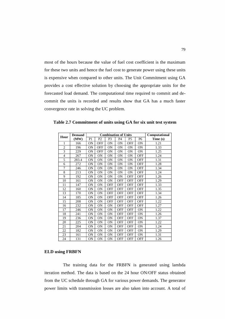
the units also varies. From the Table 2.7, it is clear that the unit P1 is ON for
24 hours because this unit generates power with minimum fuel cost as the
value of coefficient ‘A’ is minimum for this unit. Units P5 and P6 is OFF for
79
most of the hours because the value of fuel cost coefficient is the maximum
for these two units and hence the fuel cost to generate power using these units
is expensive when compared to other units. The Unit Commitment using GA
provides a cost effective solution by choosing the appropriate units for the
forecasted load demand. The computational time required to commit and de-
commit the units is recorded and results show that GA has a much faster
convergence rate in solving the UC problem.
Table 2.7 Commitment of units using GA for six unit test system
Hour Demand (MW)
Combination of Units Computational Time (s) P1 P2 P3 P4 P5 P6
1 166 ON OFF ON ON OFF ON 1.21 2 196 ON OFF ON ON ON ON 1.33 3 229 ON OFF ON ON ON ON 1.25 4 267 ON ON ON ON ON OFF 1.24 5 283.4 ON ON ON ON ON OFF 1.31 6 272 ON ON ON ON ON OFF 1.28 7 246 ON ON ON ON ON OFF 1.34 8 213 ON ON ON ON ON OFF 1.24 9 192 ON ON ON ON OFF OFF 1.26
10 161 ON ON ON OFF OFF OFF 1.29 11 147 ON ON OFF OFF OFF OFF 1.33 12 160 ON ON OFF OFF OFF OFF 1.35 13 170 ON ON OFF OFF OFF OFF 1.34 14 185 ON ON OFF OFF OFF OFF 1.26 15 208 ON ON OFF OFF OFF OFF 1.22 16 232 ON ON ON OFF OFF OFF 1.27 17 246 ON ON ON OFF OFF ON 1.22 18 241 ON ON ON OFF OFF ON 1.26 19 236 ON ON ON OFF OFF ON 1.37 20 225 ON ON ON OFF OFF ON 1.22 21 204 ON ON ON OFF OFF ON 1.24 22 182 ON ON ON OFF OFF ON 1.29 23 161 ON ON ON OFF OFF ON 1.31 24 131 ON ON ON OFF OFF OFF 1.26
ELD using FRBFN
The training data for the FRBFN is generated using lambda
iteration method. The data is based on the 24 hour ON/OFF status obtained
from the UC schedule through GA for various power demands. The generator
power limits with transmission losses are also taken into account. A total of
80
456 training samples are created in this case and 5.26% of the training data is
chosen on a trial and error basis as testing data. Figure 2.5 shows the
distribution of the initial RBF centers (stars), the selected centers (circles),
and the newly formed centers (triangles). The similarity between the newly
formed centers and the selected centers is measured and the repeating centers
are deducted in the network. The number of centers results in the number of
hidden nodes for the FRBFN algorithm. The number of hidden nodes for the 6
unit test system based on fuzzy c-means clustering is found to be 67. The
typical relationship between the number of iterations and the error rate for the
6 unit generator system is also shown in the figure. During the training
process, the error function is minimized over the given training set by
adaptively updating the parameters such as the centers, weights of the centers
and the hidden layer weights.
Figure 2.5 Clustered centers and error rate for 6 unit system
The optimized results are obtained when the FRBFN converged at
the end of 500 iterations. Table 2.8 shows the computational results of the
FRBFN for 6 unit generator system for different values of power demand
(PD). The distribution of the load among the 6 generating units (P1, P2, P3, P4,
P5, P6), the optimal fuel cost (FC), power loss (PL), total power (PT), and the
computational time (CT) are computed. The final weights w1 and w2 are
81
within the range [0.05, 0.95]. From the results it is observed that the
generating unit P1 is committed to dispatch power during the whole day,
while unit P5 generates power only during certain hours of the day. Maximum
power of 283.78MW is generated during the 5th hour, and minimum power of
131.22MW is generated during the 24th hour. The total fuel cost consumed by
the IEEE 30 bus system during a 24 hour schedule is $12967.90 with a power
loss of 13.65MW. The time taken for the algorithm to compute the results for
a single day is 23.02s.
Table 2.8 Computational results of IEEE 30 bus system using FRBFN
Hour PD (MW) Distribution of load among units (MW) FC ($/hr) PL (MW) PT
(MW) CT (s) P1 P2 P3 P4 P5 P6 1 166 112.39 0.00 24.37 16.13 0.00 13.41 446.94 0.31 166.31 0.89 2 196 132.23 0.00 19.38 10.02 14.02 20.77 541.97 0.42 196.42 0.78 3 229 173.93 0.00 17.98 10.40 12.05 15.34 649.35 0.69 229.69 0.92 4 267 151.71 80.00 15.26 10.29 10.61 0.00 742.41 0.88 267.88 1.09 5 283.4 200.00 25.96 34.29 12.95 10.58 0.00 799.90 0.38 283.78 0.99 6 272 149.77 58.31 22.78 19.02 22.88 0.00 774.84 0.75 272.75 0.89 7 246 156.98 40.63 18.81 17.43 12.85 0.00 671.28 0.71 246.71 0.99 8 213 144.58 24.62 15.27 13.21 15.87 0.00 561.09 0.55 213.55 1.03 9 192 121.42 40.71 15.45 14.88 0.00 0.00 502.43 0.46 192.46 1.03 10 161 112.55 32.66 16.17 0.00 0.00 0.00 380.84 0.39 161.39 0.85 11 147 117.85 29.55 0.00 0.00 0.00 0.00 354.62 0.39 147.39 0.99 12 160 114.54 45.89 0.00 0.00 0.00 0.00 392.61 0.43 160.43 0.99 13 170 134.46 36.06 0.00 0.00 0.00 0.00 422.57 0.52 170.52 0.98 14 185 155.93 29.71 0.00 0.00 0.00 0.00 468.70 0.64 185.64 1.05 15 208 165.07 43.71 0.00 0.00 0.00 0.00 542.23 0.78 208.78 0.89 16 232 163.15 52.08 17.59 0.00 0.00 0.00 600.30 0.82 232.82 0.99 17 246 175.26 38.96 18.63 0.00 0.00 14.03 647.33 0.88 246.88 0.86 18 241 153.34 54.10 20.03 0.00 0.00 14.31 630.54 0.78 241.78 1.04 19 236 162.80 40.99 18.85 0.00 0.00 14.13 613.78 0.78 236.78 1.11 20 225 155.64 31.74 25.31 0.00 0.00 13.01 578.72 0.70 225.70 0.98 21 204 131.51 37.86 17.09 0.00 0.00 18.07 513.42 0.54 204.54 0.90 22 182 58.96 48.63 40.49 0.00 0.00 34.21 446.92 0.29 182.29 0.96 23 161 109.67 21.00 18.15 0.00 0.00 12.53 387.65 0.34 161.35 0.97 24 131 74.23 37.22 19.77 0.00 0.00 0.00 297.46 0.22 131.22 0.86
EPSO based ELD
The Economic Load Dispatch for the committed schedules of the
IEEE 30 bus system is solved using the EPSO algorithm. The input to ELD
optimization is the UC ON/OFF schedules obtained through GA, which
provides schedule of each unit along with the generator characteristics. An
optimized power generation schedule for each hour is estimated and the
82
process is repeated for different power demands for 24 hours. The results of
ELD using EPSO algorithm are shown in Table 2.9. The generating units with
a power output of ‘0’ indicate the OFF status of the unit. Since the objective
of the UC-ELD problem is to minimize the total fuel cost, the units with
smaller cost coefficients are allocated the power first, followed by other
online units. In this test system, the most efficient unit is P1 and hence it
contributes its maximum power generating capacity for most of the load
requirement. Similarly, the units which are most expensive are allocated
minimum power thus providing improved optimal solutions.
Table 2.9 ELD results using EPSO for six unit system
Hr PD (MW)
Power generated / unit (MW) FC ($/hr)
PL (MW)
PT (MW)
CT (s) P1 P2 P3 P4 P5 P6
1 166 127.57 0 16.81 10 0 12 440.14 0.36 166.38 2.67 2 196 146.52 0 17.97 10 10 12 536.18 0.47 196.49 2.45 3 229 177.82 0 19.9 10 10 12 647.41 0.69 229.72 2.5 4 267 178.53 49.45 19.96 10 10 0 739.8 0.91 267.94 2.52 5 283.4 190.07 51.95 20.67 10 11.77 0 797.93 1.03 284.46 2.15 6 272 182.05 50.21 20.18 10 10.53 0 757.37 0.95 272.97 2.15 7 246 161.98 45.86 18.94 10 10 0 667.65 0.76 246.78 2.01 8 213 135.99 40.23 17.34 10 10 0 559.69 0.54 213.56 2.12 9 192 127.34 38.35 16.8 10 0 0 492.67 0.47 192.49 2.11 10 161 114.53 31.86 15 0 0 0 380.84 0.39 161.39 2.03 11 147 123.15 24.25 0 0 0 0 355.91 0.4 147.4 2.28 12 160 133.99 26.49 0 0 0 0 393.93 0.48 160.48 2.09 13 170 141.59 28.95 0 0 0 0 423.68 0.54 170.54 2.48 14 185 154.16 31.48 0 0 0 0 469.86 0.64 185.64 2.11 15 208 174.6 34.21 0 0 0 0 543.86 0.81 208.81 2.11 16 232 170.47 43.98 18.4 0 0 0 600.27 0.84 232.85 2.17 17 246 172.05 44.32 18.51 0 0 12 646.54 0.87 246.88 2.12 18 241 168.11 43.47 18.26 0 0 12 630.02 0.84 241.84 2.2 19 236 164.17 42.61 18.02 0 0 12 613.66 0.8 236.8 2.42 20 225 155.5 40.73 17.49 0 0 12 578.19 0.72 225.72 2.14 21 204 138.96 37.15 16.47 0 0 12 512.52 0.58 204.58 2.28 22 182 121.64 33.4 15.41 0 0 12 446.59 0.45 182.45 2.14 23 161 104.62 29.72 15 0 0 12 386.42 0.34 161.34 2.14 24 131 89.75 26.5 15 0 0 0 297.43 0.25 131.25 2.26
The fuel cost, power loss, total power and computational time of
the ELD using EPSO algorithm are computed. The total fuel cost is computed
by summing the fuel cost of each unit that is in the ‘ON’ state. It is calculated
based on the power generated by each unit and its fuel cost coefficients. From
the table it can be concluded that the total fuel cost incurred per day amounts
83
to $12918.56 and the average cost per hour is $538.27 for a total power
demand of 4953.4MW. The algorithm produced optimal results at the end of
100 iterations with the total execution time of 55.58s and mean time per hour
of 2.32s.
ELD using DE-OBL and IDE-OBL
The parameters for DE-OBL and IDE-OBL are set according to the
values shown in Table 2.4. The committed schedules obtained through GA
are dispatched using DE-OBL and IDE-OBL based on the 24 hour load
demand. The heuristic algorithms compute the power to be shared by units P1
to P6 for each load demand.
Table 2.10(a) ELD results using DE-OBL for six unit system
HOUR PD
(MW) Power generated / unit (MW) FC
($/hr) PL
(MW) PT
(MW) CT (s) P1 P2 P3 P4 P5 P6
1 166 127.55 0 16.83 10 0 12 440.14 0.36 166.38 0.55 2 196 146.66 0 17.83 10 10 12 536.19 0.47 196.49 0.62 3 229 177.9 0 19 10 10 12.81 647.57 0.7 229.71 0.5 4 267 178.91 48.4 20.27 10 10.35 0 739.83 0.91 267.93 0.56 5 283.4 187.93 52.74 21.6 10 12.18 0 798.02 1.02 284.45 0.56 6 272 181.15 50.75 20.86 10 10.2 0 757.41 0.94 272.96 0.69 7 246 166.3 45.5 15 10 10 0 668.69 0.78 246.8 0.58 8 213 138.63 38.45 16.48 10 10 0 559.82 0.55 213.56 0.53 9 192 127.51 38.3 16.69 10 0 0 492.67 0.48 192.5 0.58 10 161 114.53 31.86 15 0 0 0 380.84 0.39 161.39 0.41 11 147 115.35 32.04 0 0 0 0 354.62 0.38 147.39 0.5 12 160 126.09 34.36 0 0 0 0 392.61 0.46 160.45 0.53 13 170 134.36 36.15 0 0 0 0 422.57 0.52 170.51 0.61 14 185 146.77 38.84 0 0 0 0 468.7 0.61 185.61 0.53 15 208 165.81 42.97 0 0 0 0 542.23 0.78 208.78 0.47 16 232 170.48 43.97 18.4 0 0 0 600.27 0.84 232.85 0.48 17 246 172.3 43.48 19.09 0 0 12 646.58 0.87 246.87 0.55 18 241 167.35 43.71 18.77 0 0 12 630.04 0.83 241.83 0.62 19 236 163.85 43.08 17.86 0 0 12 613.67 0.8 236.79 0.83 20 225 156.83 39.52 17.37 0 0 12 578.23 0.72 225.72 0.61 21 204 139.5 36.93 16.16 0 0 12 512.53 0.58 204.59 0.55 22 182 121.95 33.51 15 0 0 12 446.61 0.45 182.46 0.55 23 161 104.62 29.72 15 0 0 12 386.42 0.34 161.34 0.59 24 131 89.75 26.5 15 0 0 0 297.43 0.25 131.25 0.56
A load demand of ‘0’ indicates that the unit is ‘OFF’. From the
results, it is inferred that the operating cost is proportional to the load demand.
The computed results of ELD for DE-OBL are shown in Table 2.10(a). From
84
the results it is examined that unit P1 generates a maximum power of 3522.08
MW, while a minimum power of 72.73 MW is generated by unit P5. The total
fuel cost over the 24 hour time horizon is computed by DE-OBL as
$12013.69 with a total power loss of 15.03 MW in 13.56s.
Table 2.10(b) ELD results using IDE-OBL for six unit system
HOUR PD (MW)
Power generated / unit (MW) FC ($/hr)
PL (MW)
PT (MW)
CT (s) P1 P2 P3 P4 P5 P6
1 166 127.57 0 16.81 10 0 12 437.8 0.36 166.38 0.48 2 196 146.52 0 17.97 10 10 12 534.18 0.47 196.49 0.53 3 229 177.82 0 19.90 10 10 12 643.41 0.69 229.72 0.58 4 267 178.52 49.46 19.96 10 10 0 735.8 0.91 267.94 0.58 5 283.4 200 44.64 19.84 10 10 0 774.17 1.08 284.48 0.64 6 272 200 38.05 15 10 10 0 736.77 1.04 273.05 0.59 7 246 162.04 45.83 18.90 10 10 0 657.65 0.76 246.78 0.66 8 213 135.78 40.34 17.43 10 10 0 548.69 0.54 213.56 0.59 9 192 127.41 38.29 16.79 10 0 0 483.01 0.47 192.49 0.5
10 161 114.53 31.86 15 0 0 0 361.73 0.39 161.39 0.51 11 147 115.35 32.04 0 0 0 0 350.96 0.38 147.38 0.55 12 160 126.09 34.36 0 0 0 0 381.92 0.46 160.46 0.47 13 170 134.36 36.15 0 0 0 0 401.42 0.52 170.52 0.53 14 185 146.77 38.84 0 0 0 0 449.7 0.61 185.61 0.55 15 208 165.81 42.97 0 0 0 0 531.98 0.78 208.78 0.51 16 232 170.47 43.98 18.40 0 0 0 591.27 0.84 232.84 0.5 17 246 172.02 44.35 18.50 0 0 12 632.54 0.87 246.87 0.51 18 241 168.26 43.35 18.23 0 0 12 622.02 0.84 241.84 0.5 19 236 164.48 42.48 17.84 0 0 12 604.66 0.80 236.80 0.73 20 225 155.48 40.76 17.48 0 0 12 564.19 0.72 225.72 0.59 21 204 138.88 37.18 16.52 0 0 12 508.52 0.58 204.58 0.48 22 182 121.68 33.35 15.42 0 0 12 438.59 0.45 182.45 0.58 23 161 104.62 29.72 15 0 0 12 381.28 0.34 161.34 0.56 24 131 89.75 26.50 15 0 0 0 288.44 0.25 131.25 0.48
The results for the ELD problem using IDE-OBL algorithm are
presented in Table 2.10(b). The minimum fuel cost is $288.44 for a load
demand of 131MW and the maximum fuel cost accounts to $774.17 for a load
demand of 283.4 MW. Similarly, the total power generated is maximum with
284.48MW during the 5th hour and minimum with 131.25MW during the 24th
hour. Since the transmission loss is considered in the implementation, the
total power loss of the 6 unit system over 24 hours is computed as 15.17MW.
The algorithm computed the results for all the 24 hours at the end of 13.2s.
85
ABC Results
The economic dispatch based on the on/off status of the six generating units for 24 hours load demand is determined and tabulated in Table 2.11. For each hour, load demand varies and hence the commitment of the units also varies. In ELD using ABC algorithm, the load sharing by each unit is uniformly distributed rather than allocating full load to a single unit. Thus stress in the generators can be avoided since none of the units is generating its maximum capacity. Unit P1 contributes a power of 3516.05MW, P2 generates 834.15MW, P3 delivers 336.13MW, 90MW is contributed by unit P4, unit P5 shares a load of 72.3MW and 120MW of load is generated by unit P6. Thus from the analysis, it is clear that unit P1 generates maximum power per day and unit P5 generates the minimum power. The minimum operating cost is 297.43$/hr for a load demand of
Table 2.11 Simulation results of IEEE 30 bus system using ABC
Hour PD (MW) Distribution of load among units (MW) FC ($/hr) PL (MW) PT (MW) CT (s) P1 P2 P3 P4 P5 P6
1 166 127.57 0 16.81 10 0 12 440.14 0.36 166.38 3.04 2 196 146.52 0 17.97 10 10 12 536.18 0.47 196.49 3.01 3 229 177.82 0 19.9 10 10 12 647.41 0.69 229.72 3.03 4 267 178.53 49.45 19.96 10 10 0 739.8 0.91 267.94 3.01 5 283.4 190.07 51.95 20.67 10 11.77 0 797.93 1.03 284.46 3 6 272 182.05 50.21 20.18 10 10.53 0 757.37 0.95 272.97 3.04 7 246 161.98 45.86 18.94 10 10 0 667.65 0.76 246.78 3.03 8 213 135.99 40.23 17.34 10 10 0 559.69 0.54 213.56 3.03 9 192 127.34 38.35 16.8 10 0 0 492.67 0.47 192.49 3.06 10 161 114.53 31.86 15 0 0 0 380.84 0.39 161.39 2.95 11 147 115.35 32.04 0 0 0 0 354.62 0.38 147.39 3.12 12 160 126.09 34.36 0 0 0 0 392.61 0.46 160.45 3.26 13 170 134.36 36.15 0 0 0 0 422.57 0.52 170.51 3.04 14 185 146.77 38.84 0 0 0 0 468.7 0.61 185.61 3.04 15 208 165.81 42.97 0 0 0 0 542.23 0.78 208.78 3.04 16 232 170.47 43.98 18.4 0 0 0 600.27 0.84 232.85 2.79 17 246 172.05 44.32 18.51 0 0 12 646.54 0.87 246.88 3.07 18 241 168.11 43.47 18.26 0 0 12 630.02 0.84 241.84 2.81 19 236 164.17 42.61 18.02 0 0 12 613.66 0.8 236.8 3.35 20 225 155.5 40.73 17.49 0 0 12 578.19 0.72 225.72 3.03 21 204 138.96 37.15 16.47 0 0 12 512.52 0.58 204.58 3.06 22 182 121.64 33.4 15.41 0 0 12 446.59 0.45 182.45 2.85 23 161 104.62 29.72 15 0 0 12 386.42 0.34 161.34 2.92 24 131 89.75 26.5 15 0 0 0 297.43 0.25 131.25 2.85
131 MW at the twenty fourth hour. Similarly, the maximum fuel cost
(797.9324 $/hr) is incurred during the fifth hour for a load demand of
86
283.4 MW. The total operating cost to generate power from the IEEE 30 bus system per day (24 hours) is $12912.05. The computation time required to compute the solution for 24 hour forecasted load profile is 72.43s and the mean time per hour is 3.02s.
CSO Results
Using the UC schedule from GA, for each value of power demand, the individual power generated, power loss, total power, fuel cost, and computational time are recorded by applying CSO as shown in Table 2.12. The algorithm is run for 50 trial runs, among which the best results are presented. For the given load profile of 4953.4MW, the CSO algorithm generated a total power of 4968.02MW including the transmission
losses with the fuel cost consumption of $12919.66. The entire algorithm for the 24 hour load profile consumed 15.87s to determine the results.
Table 2.12 Computational results of IEEE 30 bus system using CSO
Hour PD (MW) Distribution of load among units (MW) FC ($/hr) PL (MW) PT (MW) CT (s) P1 P2 P3 P4 P5 P6
1 166 123.72 0 15.97 11.48 0 15.19 440.76 0.34 166.36 0.75 2 196 141.91 0 20.21 10.09 10.72 13.54 536.9 0.45 196.47 0.61 3 229 176.01 0 19.27 10.47 10.27 13.69 648.76 0.68 229.71 0.62 4 267 166.89 53 24.5 12.01 11.45 0 740.31 0.84 267.85 0.69 5 283.4 176.52 34.97 37.09 17.59 18.11 0 799.07 0.84 284.28 0.66 6 272 180.85 46.3 21.88 10.12 13.8 0 758.18 0.92 272.95 0.69 7 246 156.8 48.21 18.6 11.98 11.16 0 668.12 0.72 246.75 0.58 8 213 138.78 32.51 18.73 12.13 11.4 0 560.29 0.52 213.55 0.67 9 192 125.26 36.66 19.82 10.73 0 0 493.26 0.46 192.47 0.61
10 161 114.2 31.75 15.44 0 0 0 380.84 0.39 161.39 0.69 11 147 119.95 27.45 0 0 0 0 354.62 0.4 147.4 0.69 12 160 126.03 34.43 0 0 0 0 392.61 0.46 160.46 0.64 13 170 134.29 36.22 0 0 0 0 422.57 0.52 170.51 0.69 14 185 147.23 38.38 0 0 0 0 468.7 0.62 185.61 0.62 15 208 165.81 42.97 0 0 0 0 542.23 0.78 208.78 0.69 16 232 168.35 44.29 20.19 0 0 0 600.27 0.83 232.83 0.81 17 246 161.17 41.2 22.45 0 0 21.97 646.68 0.79 246.79 0.67 18 241 155.99 53.25 19.45 0 0 13.1 630.05 0.79 241.79 0.69 19 236 157.76 48.5 18.41 0 0 12.11 613.8 0.78 236.78 0.64 20 225 149.3 38.32 24.7 0 0 13.35 578.24 0.68 225.67 0.67 21 204 146.06 28.03 17.96 0 0 12.54 512.65 0.6 204.59 0.66 22 182 121.38 33.78 15.24 0 0 12.06 446.64 0.45 182.46 0.61 23 161 102.34 30.75 16.16 0 0 12.09 386.67 0.33 161.34 0.58 24 131 77.24 38.12 15.87 0 0 0 297.44 0.23 131.23 0.64
87
2.4.3 Case Study II – Ten Unit Test System
The second case study consists of a ten unit test system (Park et al
2010). The input data includes the generator limits, fuel cost coefficients,
transmission loss matrix and load profile for 24 hours. The minimum
generating capacity of the system is 690 MW and the maximum generating
capacity is 2358 MW. The load profile and the generator input data and the
variation of load for 24 hours per day is given in Tables A1.4 to A1.6 in
Appendix 1. The minimum power demand requirement is 1036 MW and the
maximum demand is 2220 MW. The committed schedules of the ten unit
system obtained through GA are further dispatched using the proposed
intelligent heuristics. The results and discussions of FRBFN, EPSO,
DE-OBL, IDE-OBL, ABC and CSO are elaborated in this section.
Committed Schedules using GA
Genetic algorithm is applied to obtain the optimal solution of the
unit commitment problem. In each generation, individuals are tested for load
demand and unit constraints. These individuals are weighted according to
their constraint satisfactions. Worst individuals are weighted with a very high
factor so that they will have less chance in competition during the next
generation. The process is repeated until a predefined number of generations
have reached. The GA parameters and their settings are shown in Table 2.1.
The 10 unit system is solved using GA for obtaining the unit commitment
schedules based on the load demand for 24 hours. The forecasted loads,
committed schedules and the computational time are shown in Table 2.13. In
the table, the committed/de-committed status is represented in terms of
ON/OFF and this indicates the number of generating units that are committed
during the 24 hour schedule depending upon the demand. It is observed from
the table that unit P1 is kept ON throughout the day because this unit
generates power with minimum fuel cost as the cost coefficient ‘A’ is
88
minimum for this unit. Similarly unit P8 is the most expensive unit and hence
it is kept OFF during most hours of the day. In general, small units can be
committed/de-committed at short intervals. The on-times of these units must
be minimized since the operational cost required on these units is too
expensive. Thus in unit commitment the order of commitment is determined
based on the cost characteristics.
Table 2.13 Unit commitment schedule for 10 unit test system
Hour Demand (MW)
Combination of units Computational Time (s) P1 P2 P3 P4 P5 P6 P7 P8 P9 P10
1 1036 ON OFF OFF ON OFF ON ON OFF OFF ON 2.08 2 1110 ON OFF OFF ON ON ON OFF OFF OFF OFF 2.15 3 1258 ON ON ON OFF OFF OFF OFF OFF OFF ON 2.31 4 1406 ON ON OFF ON OFF ON OFF OFF ON ON 2.11 5 1480 ON ON ON OFF ON OFF OFF OFF ON OFF 2.35 6 1628 ON ON ON OFF ON ON OFF OFF OFF ON 2.18 7 1702 ON ON ON ON OFF ON OFF OFF OFF ON 2.19 8 1776 ON ON ON ON ON OFF OFF OFF OFF OFF 2.17 9 1924 ON ON ON ON ON ON OFF OFF OFF ON 2.09 10 2072 ON ON ON ON ON ON ON OFF OFF OFF 2.34 11 2146 ON ON ON ON ON ON ON ON OFF OFF 2.26 12 2220 ON ON ON ON ON ON ON OFF ON ON 2.18 13 2072 ON ON ON ON ON ON ON OFF OFF OFF 2.22 14 1924 ON ON ON ON ON ON OFF OFF OFF ON 2.25 15 1776 ON ON ON ON ON OFF OFF OFF OFF OFF 2.24 16 1554 ON ON ON OFF ON OFF ON OFF OFF OFF 2.31 17 1480 ON ON ON OFF ON OFF OFF OFF ON OFF 2.27 18 1628 ON ON ON OFF ON ON OFF OFF OFF ON 2.29 19 1776 ON ON ON ON ON OFF OFF OFF OFF OFF 2.11 20 2072 ON ON ON ON ON ON ON OFF OFF OFF 2.35 21 1924 ON ON ON ON ON ON OFF OFF OFF ON 2.33 22 1628 ON ON ON OFF ON ON OFF OFF OFF ON 2.24 23 1332 ON ON OFF OFF ON OFF OFF ON ON ON 2.16 24 1184 ON ON OFF OFF OFF OFF OFF ON ON ON 2.06
FRBFN based ELD
The structural design of the FRBFN is modified for 10 unit test
system with three input nodes and ten output nodes. The ten output nodes
correspond to optimal power generated for each generating unit and three
input nodes represent weights w1 and w2, and power demand. The number of
hidden nodes determined using the fuzzy c-means algorithm is found to be 64
for the 10 unit system. The FRBFN network is trained with 456 patterns
89
generated through LIM method for 500 iterations with network parameters
initialized as shown in Table 2.2. The clustered centers and error rate for the
ten unit test system using FRBFN is shown in Figure 2.6. Among the number
of clustered centers, 64 centers are selected (triangles) as hidden units in
random with a learning rate of 0.997 and step size of 0.002. The rate of
change of error implies that the algorithm converges to a constant error rate of
0.0840 from its initial value of 3.8128.
Figure 2.6 Clustered centers and error rate for 10 unit system
The economic dispatch results using FRBFN for ten unit test
system such as the distribution of load among committed units, fuel cost,
power generated in each unit, power loss, total power and computational time
for various values of power demand over the 24 hour schedule is shown in
Tables 2.14(a) and 2.14(b). From the results it is examined that unit P1
generates a maximum power of 10677MW, while a minimum power of
330.4MW is generated by unit P8. The total fuel cost over the 24 hour time
horizon is computed by the FRBFN as $973453.4 with a total power loss of
95.29MW. In general, neural networks take a longer time to train more
samples and in this case study it is observed to be 88.53s.
90
Table 2.14(a) Optimal dispatch using FRBFN for ten unit test system
Hr PD (MW)
Distribution of load among units (MW) P1 P2 P3 P4 P5 P6 P7 P8 P9 P10
1 1036 432.7 0 0 261.2 0 160 129.6 0 0 55 2 1110 457.9 0 0 252.3 243 160 0 0 0 0 3 1258 406.1 460 340 0 0 0 0 0 0 55 4 1406 428.6 460 0 238.2 0 160 0 0 69.1 55 5 1480 360.7 460 340 0 243 0 0 0 80 0 6 1628 375.9 459.9 340 0 241.5 160 0 0 0 55 7 1702 462.4 460 340 231 0 157.8 0 0 0 55 8 1776 470 425.98 340 300 243 0 0 0 0 0 9 1924 470 361.2 340 300 243 160 0 0 0 55
10 2072 454.3 460 340 298.5 234.8 159.8 130 0 0 0 11 2146 461 460 340 243.7 243 160 130 113.6 0 0 12 2220 470 460 340 300 227.6 160 130 0 80 55 13 2072 449.2 460 340 295.3 243 160 130 0 0 0 14 1924 454.7 436.8 340 267.5 213.4 160 0 0 0 55 15 1776 470 460 340 284.7 226.75 0 0 0 0 0 16 1554 386.8 460 340 0 241.8 0 130 0 0 0 17 1480 470 460 245.4 0 229.3 0 0 0 78.8 0 18 1628 470 452.7 340 0 194.3 119.2 0 0 0 55 19 1776 435.5 460 340 300 243 0 0 0 0 0 20 2072 470 460 340 300 243 134.56 130 0 0 0 21 1924 470 460 340 296.3 222.5 86 0 0 0 55 22 1628 413.6 460 340 0 202 160 0 0 0 55 23 1332 467.6 452.4 0 0 228 0 0 96.8 37 55 24 1184 470 460 0 0 0 0 0 120 80 55
Table 2.14(b) Optimal dispatch using FRBFN for ten unit test system
Hour PD (MW) FC ($/hr) PL (MW) PT (MW) CT (s) 1 1036 25241.95 2.5 1038.5 3.56 2 1110 26741.91 3.2 1113.2 3.47 3 1258 30617.19 3.1 1261.1 3.44 4 1406 35175.16 4.9 1410.9 3.98 5 1480 35684.98 3.7 1483.7 3.54 6 1628 39174.4 4.3 1632.3 3.58 7 1702 41318.94 4.2 1706.2 2.99 8 1776 42801.05 2.98 1778.98 4.01 9 1924 46755.05 5.2 1929.2 4.08 10 2072 49141.77 5.4 2077.4 3.96 11 2146 51480.3 5.3 2151.3 3.45 12 2220 54130.16 2.6 2222.6 4.05 13 2072 49130.38 5.5 2077.5 3.87 14 1924 46617.37 3.4 1927.4 3.77 15 1776 42724.69 5.45 1781.45 3.21 16 1554 36669.89 4.6 1558.6 3.41 17 1480 35656.16 3.5 1483.5 3.48 18 1628 39136.83 3.2 1631.2 3.89 19 1776 42768.71 2.5 1778.5 4.11 20 2072 49109.59 5.56 2077.56 3.74 21 1924 46609.94 5.8 1929.8 3.56 22 1628 39136.72 2.6 1630.6 3.82 23 1332 33788.15 4.8 1336.8 3.91 24 1184 33842.08 1 1185 3.65
ELD using EPSO
In this case study, ten units are committed to serve a 24 hour load
pattern using GA. The parameters of EPSO are set according to Table 2.3.
91
Based on the GA committed schedules, the EPSO computes the load
distribution among each unit for every hour. The experimental results are
shown in Tables 2.15(a) and 2.15(b). From the tables, it can be inferred that
the units P1 and P3 are allocated the maximum load if they are in ON state.
This is because the fuel cost coefficient of these two units is minimum and
hence they are highly economical. Unit P10 is always allocated 55MW
because its maximum and minimum generator limits are the same. For units
P3, P6 and P7, maximum power is allocated for all values of load demand.
Analyzing other units such as P2, P4, P5, P8 and P9, reveals that the load is
allocated to these units according to the load demand and the unit
commitment schedule. The maximum fuel cost of $53970.94 is incurred for a
load demand of 2220 MW during the 12th hour and the minimum fuel cost
($25175.96) is incurred during the 1st hour for a load demand of 1036 MW.
The total operating cost for a day amounts to $972282.3 and the mean cost
per hour is $40511.76. EPSO algorithm takes 59.14 seconds to obtain the
ELD results for 24 hours.
Table 2.15(a) ELD results using EPSO for ten unit system
HOUR Power generated / unit (MW) P1 P2 P3 P4 P5 P6 P7 P8 P9 P10
1 470 0 0 223.57 0 160 130 0 0 55 2 470 0 0 240.29 243 160 0 0 0 0 3 406.10 460 340 0 0 0 0 0 0 55 4 470 460 0 245.20 0 160 0 0 20.89 55 5 439.32 460 340 0 224.46 0 0 0 20 0 6 411.56 460 340 0 205.66 160 0 0 0 55 7 470 460 340 221.19 0 160 0 0 0 55 8 470 460 340 267.20 243 0 0 0 0 0 9 470 460 340 201.00 243 160 0 0 0 55 10 470 460 340 274.56 243 160 130 0 0 0 11 469.97 459.98 340 254.67 243 160 130 93.75 0 0 12 470 460 340 300 243 160 130 0 68.38 55 13 469.89 459.82 340 275.06 242.86 159.97 129.95 0 0 0 14 470 460 340 199.38 243 160 0 0 0 55 15 470 460 340 265.62 243 0 0 0 0 0 16 417.15 460 340 0 211.41 0 130 0 0 0 17 438.34 460 340 0 223.84 0 0 0 20 0 18 410.57 460 340 0 205.03 160 0 0 0 55 19 470 460 340 265.62 243 0 0 0 0 0 20 470 460 340 272.98 243 160 130 0 0 0 21 469.98 460 340 199.40 243 160 0 0 0 55 22 410.56 460 340 0 205.03 160 0 0 0 55 23 470 460 0 0 243 0 0 88.50 20.44 55 24 470 460 0 0 0 0 0 120 80 55
92
Table 2.15(b) ELD results using EPSO for ten unit system
Hour PD (MW) FC ($/hr) PL (MW) PT (MW) CT (s) 1 1036 25175.96 2.57 1038.57 2.82 2 1110 26715.95 3.29 1113.29 2.59 3 1258 30617.19 3.10 1261.10 2.40 4 1406 35057.52 5.09 1411.09 2.43 5 1480 35649.50 3.77 1483.77 2.57 6 1628 39172.35 4.22 1632.22 2.37 7 1702 41289.07 4.19 1706.19 2.50 8 1776 42748.83 4.20 1780.20 2.48 9 1924 46581.09 5.00 1929.00 2.39 10 2072 49087.52 5.56 2077.56 2.51 11 2146 51463.10 5.37 2151.37 2.37 12 2220 53970.94 6.37 2226.37 2.29 13 2072 49089.03 5.56 2077.56 2.50 14 1924 46541.86 3.38 1927.38 2.57 15 1776 42710.37 2.62 1778.62 2.42 16 1554 36669.74 4.56 1558.56 2.48 17 1480 35614.59 2.19 1482.19 2.43 18 1628 39136.72 2.60 1630.60 2.37 19 1776 42710.37 2.62 1778.62 2.84 20 2072 49049.03 3.98 2075.98 2.36 21 1924 46541.91 3.38 1927.38 2.20 22 1628 39136.72 2.60 1630.60 2.36 23 1332 33710.85 4.94 1336.94 2.50 24 1184 33842.08 4.33 1185.00 2.39
ELD using DE-OBL and IDE-OBL
The OBL based DE and IDE are used to determine the optimal
dispatch of the GA committed schedules for the ten unit system. The
parameters and their values are set according to Table 2.4. The population
size for the ten unit system is set to 40, crossover probability to 0.6 and step
size to 0.8 respectively. Since DE-OBL uses only one set of population during
the entire run, the algorithm is capable of attaining a faster convergence rate,
thus reducing the computational time. The computed optimal results for DE-
OBL are shown in Tables 2.16(a) and 2.16(b). The total power demand
requirement for the 10 unit system is 40108 MW. Unit P1 generated a
maximum power of 10574.51 MW and unit P9 generated a minimum power
of 240 MW over the 24 hours. The optimal cost for generating the total power
including the transmission losses is $ 973049.1.
93
Table 2.16(a) ELD results using DE-OBL for ten unit system
Hour Power generated / unit (MW)
P1 P2 P3 P4 P5 P6 P7 P8 P9 P10 1 470 0 0 223.57 0 160 130 0 0 55 2 446.87 0 0 263.33 243 160 0 0 0 0 3 406.10 460 340 0 0 0 0 0 0 55 4 436.44 460 0 279.52 0 160 0 0 20 55 5 420.78 460 340 0 243 0 0 0 20 0 6 398.73 460 340 0 218.50 160 0 0 0 55 7 431.71 460 340 259.40 0 160 0 0 0 55 8 455.09 460 340 282.06 243 0 0 0 0 0 9 451.39 460 340 219.56 243 160 0 0 0 55 10 462.22 460 340 300 225.27 160 130 0 0 0 11 458.42 460 340 300 243 160 130 60.07 0 0 12 458.38 460 340 300 243 160 130 0 80 55 13 444.49 460 340 300 243 160 130 0 0 0 14 437.37 460 340 231.93 243 160 0 0 0 55 15 465.94 460 340 269.67 243 0 0 0 0 0 16 385.58 460 340 0 243 0 130 0 0 0 17 419.20 460 340 0 243 0 0 0 20 0 18 408.83 460 340 0 206.77 160 0 0 0 55 19 450.69 460 340 284.86 243 0 0 0 0 0 20 466.27 460 340 276.70 243 160 130 0 0 0 21 455.93 460 340 213.41 243 160 0 0 0 55 22 410.08 460 340 0 205.52 160 0 0 0 55 23 464 460 0 0 243 0 0 94.89 20 55 24 470 460 0 0 0 0 0 120 80 55
Table 2.16(b) ELD results using DE-OBL for ten unit system
Hour PD (MW) FC ($/hr) PL (MW) PT (MW) CT (s) 1 1036 25175.97 2.57 1038.57 0.90 2 1110 26765.92 3.19 1113.19 0.73 3 1258 30617.19 3.10 1261.10 0.61 4 1406 35131.00 4.96 1410.96 0.83 5 1480 35650.05 3.78 1483.78 0.58 6 1628 39172.61 4.23 1632.23 0.70 7 1702 41373.02 4.10 1706.10 0.94 8 1776 42781.70 4.15 1780.15 0.73 9 1924 46620.78 4.95 1928.95 0.66 10 2072 49144.65 5.49 2077.49 0.59 11 2146 51503.09 5.49 2151.49 0.62 12 2220 54130.94 6.38 2226.38 0.62 13 2072 49144.65 5.49 2077.49 0.90 14 1924 46612.04 3.30 1927.30 0.72 15 1776 42719.26 2.60 1778.60 0.61 16 1554 36671.32 4.58 1558.58 0.83 17 1480 35615.17 2.20 1482.20 0.55 18 1628 39136.72 2.60 1630.60 0.72 19 1776 42753.02 2.55 1778.55 0.89 20 2072 49057.26 3.97 2075.97 0.86 21 1924 46571.75 3.34 1927.34 0.62 22 1628 39136.72 2.60 1630.60 0.59 23 1332 33722.23 4.89 1336.89 0.95 24 1184 33842.08 4.33 1185.00 0.69
94
Table 2.16(c) Economic dispatch using IDE-OBL for ten unit system
Hour Power generated / unit (MW)
P1 P2 P3 P4 P5 P6 P7 P8 P9 P10 25 469.99 0 0 223.57 0 160 130 0 0 55 26 470 0 0 240.29 243 160 0 0 0 0 27 406.10 460 340 0.00 0 0 0 0 0 55 28 469.89 460 0 246.20 0 160 0 0 20 55 29 440.19 460 340 0 223.58 0 0 0 20 0 30 411.56 460 340 0 205.66 160 0 0 0 55 31 470.00 460 340 221.19 0 160 0 0 0 55 32 469.96 460 340 267.24 243 0 0 0 0 0 33 470 460 340 201.00 243 160 0 0 0 55 34 469.67 460 340 274.89 243 160 130 0 0 0 35 467.47 460 340 230.78 243 160 130 120 0 0 36 469.86 460 340 300 243 160 130 0 68.51 55 37 455.27 460 340 300 232.22 160 130 0 0 0 38 469.99 460 340 199.39 243 160 0 0 0 55 39 470 460 340 265.62 243 0 0 0 0 0 40 417.15 460 340 0.00 211.41 0 130 0 0 0 41 419.20 460 340 0.00 243 0 0 0 20 0 42 410.56 460 340 0.00 205.04 160 0 0 0 55 43 469.70 460 340 265.92 243 0 0 0 0 0 44 464.54 460 340 278.43 243 160 130 0 0 0 45 470.00 460 340 199.38 243 160 0 0 0 55 46 410.56 460 340 0 205.03 160 0 0 0 55 47 469.84 460 0 0 243 0 0 89.10 20 55 48 470 460 0 0 0 0 0 120 80 55
Table 2.16(d) Economic dispatch using IDE-OBL for ten unit system
Hour PD (MW) FC ($/hr) PL (MW) PT (MW) CT (s) 1 1036 25161.96 2.57 1038.57 0.61 2 1110 26715.95 3.29 1113.29 0.56 3 1258 30603.24 3.10 1261.10 0.47 4 1406 35057.97 5.09 1411.09 0.58 5 1480 35639.5 3.77 1483.77 0.59 6 1628 39159.35 4.22 1632.22 0.55 7 1702 41289.07 4.19 1706.19 0.58 8 1776 42748.92 4.20 1780.20 0.55 9 1924 46571.09 5.00 1929.00 0.53 10 2072 49088.25 5.56 2077.56 0.62 11 2146 51466.27 5.26 2151.26 0.56 12 2220 53972.63 6.37 2226.37 0.66 13 2072 49121.53 5.49 2077.49 0.59 14 1924 46541.89 3.38 1927.38 0.66 15 1776 42710.37 2.62 1778.62 0.51 16 1554 36669.74 4.56 1558.56 0.55 17 1480 35588.17 2.20 1482.20 0.59 18 1628 39124.75 2.60 1630.60 0.55 19 1776 42711.04 2.62 1778.62 0.87 20 2072 49046.17 3.96 2075.96 0.62 21 1924 46527.86 3.38 1927.38 0.67 22 1628 39118.16 2.60 1630.60 0.66 23 1332 33710.18 4.94 1336.94 0.69 24 1184 33814.52 4.33 1185.00 0.59
95
The load distribution among the ten individual generating units,
fuel cost, power loss, total power and computational time are evaluated
through IDE-OBL and shown in Tables 2.16(c) and 2.16(d). For an overall
power requirement of 40108MW, the IDE-OBL algorithm dispatches the
power among all the ten units with a total cost consumption of $972158.58,
including a power loss of 95.3 MW taking a time of 14.4s.
ABC Results
The impact of ABC for obtaining optimal dispatch of the
committed schedules is analyzed in this section. The parameters are set
according to Table 2.5. The experimental results for the ten unit system based
on ABC are shown in Tables 2.17(a) and 2.17(b).
Table 2.17(a) Optimal dispatch using ABC for ten unit test system
Hr PD (MW)
Distribution of load among units (MW) P1 P2 P3 P4 P5 P6 P7 P8 P9 P10
1 1036 470 0 0 223.57 0 160 130 0 0 55 2 1110 470 0 0 240.29 243 160 0 0 0 0 3 1258 406.10 460 340 0 0 0 0 0 0 55 4 1406 470 460 246.10 0 160 0 0 20 55 5 1480 439.32 460 340 0 224.46 0 0 0 20 0 6 1628 411.56 460 340 0 205.66 160 0 0 0 55 7 1702 470 460 340 221.19 0 160 0 0 0 55 8 1776 470 460 340 267.79 242.41 0 0 0 0 0 9 1924 470 460 340 201.93 242.07 160 0 0 0 55
10 2072 470 460 340 274.56 243.00 160 130 0 0 0 11 2146 469.06 460 340 254.07 238.81 160 130 99.40 0 0 12 2220 469.78 460 340 298.12 243.00 160 130 0 70.48 55 13 2072 470 460 340 274.56 243.00 160 130 0 0 0 14 1924 470 460 340 200.28 242.10 160 0 0 0 55 15 1776 470 460 340 266.21 242.41 0 0 0 0 0 16 1554 417.15 460 340 0 211.41 0 130 0 0 0 17 1480 438.34 460 340 0 223.84 0 0 0 20 0 18 1628 410.56 460 340 0 205.04 160 0 0 0 55 19 1776 470 460 340 266.20 242.42 0 0 0 0 0 20 2072 470 460 340 272.98 243.00 160 130 0 0 0 21 1924 469.91 460 340 200.21 242.26 160 0 0 0 55 22 1628 410.56 460 340 0 205.04 160 0 0 0 55 23 1332 469.83 460 0 0 243.00 0 0 89.11 20 55 24 1184 470 460 0 0 0 0 0 120 80 55
Unit P1 is kept ON for the entire day because it has the minimum
fuel cost coefficients and hence it also generates the maximum power per day.
Unit P8 is the most expensive unit with a fuel cost coefficient of 0.0048
96
($/MW-h2). For units P2, P3, P6 and P7, maximum generation limit is allocated
for all load demands. For units P4, P5, P8 and P9, the load sharing is allotted
based on the load demand and combination of units in ON state. For each load
demand in the 24 hour load profile, the power generated by each unit varies
according to their fuel cost function, generating limits and also the UC schedule.
Unit P1 generates a load of 10922.16MW per day whereas unit P8 shares a load
of only 308.51MW per day.
Table 2.17(b) Optimal dispatch using ABC for ten unit test system
Hour PD (MW) FC ($/hr) PL (MW) PT (MW) CT (s)
1 1036 25175.96 2.57 1038.57 3.63
2 1110 26715.95 3.29 1113.29 3.67
3 1258 30617.19 3.10 1261.10 3.43
4 1406 35057.74 5.09 1411.09 3.82
5 1480 35649.50 3.77 1483.77 3.76
6 1628 39172.35 4.22 1632.22 3.63
7 1702 41289.07 4.19 1706.19 3.99
8 1776 42750.11 4.20 1780.20 3.39
9 1924 46583.04 5.00 1929.00 3.84
10 2072 49087.52 5.56 2077.56 3.92
11 2146 51473.08 5.34 2151.34 3.92
12 2220 53993.48 6.38 2226.38 3.84
13 2072 49087.52 5.56 2077.56 3.63
14 1924 46543.77 3.38 1927.38 3.99
15 1776 42711.67 2.61 1778.61 3.49
16 1554 36669.74 4.56 1558.56 3.51
17 1480 35614.59 2.19 1482.19 3.92
18 1628 39136.72 2.60 1630.60 3.82
19 1776 42711.65 2.61 1778.61 3.96
20 2072 49049.03 3.98 2075.98 4.07
21 1924 46543.62 3.38 1927.38 3.53
22 1628 39136.72 2.60 1630.60 3.48
23 1332 33711.18 4.94 1336.94 3.98
24 1184 33842.08 4.33 1185.00 3.71
It can be concluded that unit P1 shares the maximum load which
accounts to 27.17% of the total load demand per day and P9 shares the
minimum power of 0.76% of the total demand. The execution time of the
97
algorithm for generating the schedule for 24 hours is 89.93s and the average time
per hour is 3.75s.
CSO for ELD
The parameter setting for the CSO is not a challenging task since
the algorithm has a very few parameters to be set. The parameters and their
settings are chosen according to Table 2.6. For each value of power demand
over the 24 hour schedule, the individual power generated, power loss, total
power, fuel cost, and computational time (CT) are recorded as shown in
Tables 2.18(a) and 2.18(b).
Table 2.18(a) Optimal dispatch using CSO for ten unit test system
Hr PD (MW) Distribution of load among units (MW)
P1 P2 P3 P4 P5 P6 P7 P8 P9 P10 1 1036 413.05 0.00 0.00 280.27 0.00 160.00 130.00 0.00 0.00 55.00 2 1110 410.07 0.00 0.00 300.00 243.00 160.00 0.00 0.00 0.00 0.00 3 1258 470.00 460.00 243.71 0.00 0.00 0.00 0.00 0.00 0.00 55.00 4 1406 470.00 147.98 0.00 232.26 0.00 158.93 0.00 0.00 55.07 55.00 5 1480 401.40 460.00 340.00 0.00 243.00 0.00 0.00 0.00 39.35 0.00 6 1628 470.00 460.00 340.00 0.00 89.80 86.29 0.00 0.00 0.00 55.00 7 1702 470.00 460.00 340.00 300.00 0.00 70.34 0.00 0.00 0.00 55.00 8 1776 470.00 460.00 340.00 230.22 243.00 0.00 0.00 0.00 0.00 0.00 9 1924 470.00 268.32 340.00 253.65 243.00 99.29 0.00 0.00 0.00 55.00
10 2072 470.00 328.52 340.00 172.73 188.86 118.19 85.49 0.00 0.00 0.00 11 2146 470.00 460.00 168.47 253.54 134.02 93.45 59.59 71.61 0.00 0.00 12 2220 458.38 460.00 340.00 300.00 243.00 160.00 130.00 0.00 80.00 55.00 13 2072 464.38 460.00 340.00 283.66 240.82 160.00 128.68 0.00 0.00 0.00 14 1924 369.65 460.00 340.00 300.00 243.00 159.57 0.00 0.00 0.00 55.00 15 1776 464.28 460.00 340.00 271.32 243.00 0.00 0.00 0.00 0.00 0.00 16 1554 385.58 460.00 340.00 0.00 243.00 0.00 130.00 0.00 0.00 0.00 17 1480 470.00 275.77 340.00 0.00 155.29 0.00 0.00 0.00 24.60 0.00 18 1628 410.72 460.00 340.00 0.00 204.88 160.00 0.00 0.00 0.00 55.00 19 1776 470.00 322.58 227.10 267.22 171.79 0.00 0.00 0.00 0.00 0.00 20 2072 443.85 460.00 340.00 299.14 242.91 160.00 130.00 0.00 0.00 0.00 21 1924 470.00 460.00 210.28 143.18 224.02 160.00 0.00 0.00 0.00 55.00 22 1628 437.03 460.00 340.00 0.00 178.57 160.00 0.00 0.00 0.00 55.00 23 1332 470.00 421.39 0.00 0.00 218.63 0.00 0.00 112.09 32.63 55.00 24 1184 470.00 460.00 0.00 0.00 0.00 0.00 0.00 120.00 80.00 55.00
98
Table 2.18(b) Optimal dispatch using CSO for ten unit test system
Hour PD (MW) FC ($/hr) PL (MW) PT (MW) CT (s) 1 1036 25239.66 2.32 1038.32 0.66 2 1110 26718.75 3.07 1113.07 0.73 3 1258 30617.19 3.43 1228.71 0.67 4 1406 35081.06 3.15 1119.24 0.62 5 1480 35654.55 3.75 1483.75 0.73 6 1628 39172.35 3.80 1501.09 0.69 7 1702 41294.21 3.97 1695.34 0.89 8 1776 42784.72 4.13 1743.22 0.67 9 1924 46594.21 3.52 1729.26 0.69 10 2072 49087.91 3.63 1703.79 0.64 11 2146 51516.20 4.39 1710.69 0.76 12 2220 54117.43 6.38 2226.38 0.89 13 2072 49105.50 5.53 2077.53 0.83 14 1924 46645.15 3.21 1927.21 0.97 15 1776 42722.90 2.60 1778.60 0.90 16 1554 36669.74 4.58 1558.58 0.80 17 1480 35615.36 1.94 1265.66 0.98 18 1628 39136.72 2.60 1630.60 0.90 19 1776 42713.89 2.22 1458.70 0.76 20 2072 49099.79 3.90 2075.90 0.67 21 1924 46599.10 3.13 1722.48 1.03 22 1628 39136.73 2.60 1630.60 0.92 23 1332 33723.31 4.46 1309.75 0.92 24 1184 33842.08 4.33 1185.00 0.90
From the results, it is determined that for a minimum load demand
of 1036 MW, the fuel cost is $25239.66 during the first hour and the fuel cost
is $54117.43 for the maximum load demand of 2220 MW during the twelfth
hour. The total fuel cost to generate a power of 40108 MW per day is
$972888.5. The computational time of the CSO algorithm for generating the
schedule for 24 hours is 19.23s and the average time per hour is 0.8s.
2.4.4 Case Study III – Fifteen Unit Test System
The Indian utility 75-bus Uttar Pradesh State Electricity Board
(UPSEB) system with fifteen generating units is chosen as the test system for
analysis of commitment and optimal dispatch (Prabhakar et al 2009). The load
demand, characteristics of generators, and loss coefficients are given in
Tables A1.7 to A1.9 in Appendix 1. The experimental analysis and effect of
the intelligent techniques on the Indian utility 75-bus system is delineated in
this section.
99
UC using GA
For every hour during the 24 hour schedule, all the possible
combinations that satisfy the load demand constraints are selected and these
states are allowed to perform the optimal power flow. This procedure is
continued for the specified time horizon until all the units in the test system
are committed/de-committed. The complete unit commitment schedule is
obtained and the power is dispatched in an optimal manner using FRBFN,
EPSO, DE-OBL, IDE-OBL, ABC and CSO algorithms.
Table 2.19 Unit commitment schedule for fifteen unit system using GA
Hour Demand (MW)
Combination of units Time (s) P1 P2 P3 P4 P5 P6 P7 P8 P9 P10 P11 P12 P13 P14 P15
1 3352 1 1 1 1 1 0 1 1 1 1 1 1 1 1 1 3.14 2 3384 1 1 1 1 1 0 0 0 1 1 1 1 1 1 1 3.56 3 3437 1 1 1 1 1 0 1 0 1 1 1 1 1 1 1 3.99 4 3489 1 1 1 1 1 0 1 0 1 1 1 1 1 1 1 3.98 5 3659 1 1 1 1 1 0 1 0 1 1 1 1 1 1 1 3.78 6 3849 1 1 1 1 1 0 1 0 1 1 1 1 1 1 1 3.65 7 3898 1 1 1 1 1 0 1 0 1 1 1 1 1 1 1 3.74 8 3849 1 1 1 1 1 0 1 0 1 1 1 1 1 1 1 3.81 9 3764 1 1 1 1 1 0 1 0 1 1 1 1 1 1 1 3.94
10 3637 1 1 1 1 1 0 1 0 1 1 1 1 1 1 1 3.82 11 3437 1 1 1 1 1 0 1 0 1 1 1 1 1 1 1 3.86 12 3384 1 1 1 1 1 0 0 0 1 1 1 1 1 1 1 3.88 13 3357 1 1 1 1 1 0 0 0 1 1 1 1 1 1 1 3.87 14 3394 1 1 1 1 1 0 0 0 1 1 1 1 1 1 1 3.74 15 3616 1 1 1 1 1 0 0 0 1 1 1 1 1 1 1 3.61 16 3828 1 1 1 1 1 0 0 0 1 1 1 1 1 1 1 3.96 17 3828 1 1 1 1 1 0 0 0 1 1 1 1 1 1 1 3.54 18 3786 1 1 1 1 1 0 0 0 1 1 1 1 1 1 1 3.83 19 3659 1 1 1 1 1 0 0 0 1 1 1 1 1 1 1 3.72 20 3458 1 1 1 1 1 0 0 0 1 1 1 1 1 1 1 3.81 21 3394 1 1 1 1 1 0 0 0 1 1 1 1 1 1 1 3.88 22 3334 1 1 1 1 1 0 0 0 1 1 1 1 1 0 1 3.76 23 3329 1 1 1 1 1 0 0 0 1 1 1 1 1 0 1 3.99 24 3348 1 1 1 1 1 0 0 0 1 1 1 1 1 0 1 3.58
The ON/OFF schedule represented in binary form 1/0 for the Indian
utility 75-bus 15 unit system is shown in Table 2.19. All units in the system
are committed to serve the load demand for the whole day except for units P7,
P8 and P14. Unit P6 is not committed during any hour, since operating this unit
is too expensive due to the high values of cost coefficients.
100
FRBFN based ELD
The different combinations of the committed/de-committed
schedules obtained through GA are dispatched using lambda iteration method
(LIM) to determine the fuel cost, individual power generated, power loss, and
total power. The training data for the FRBFN is generated based on LIM. A
total of 456 training patterns are generated and among these 48 patterns are
chosen as testing samples. The parameters used for the FRBFN are shown in
Table 2.2. The difference between the target and trained input is computed as
the error. The algorithm terminates if the error is less than the tolerance value.
More accurate results are produced with proper selection of training data. It
should also be ensured that the training data are uniformly distributed, so that
the network converges faster with optimal and quality solution.
Figure 2.7 Clustered centers and error rate for 15 unit system
Figure 2.7 shows the chosen centers (triangles) after applying the
fuzzy c-means clustering algorithm and the error rate at which the algorithm
converges. The number of centers is found to be 63 after performing the
clustering operation and the error rate at which the clustering converged is
101
observed as 0.0453 (initially it is 2.0715) with respect to the number of
iterations.
Table 2.20(a) Optimal dispatch using FRBFN for fifteen unit test system
Hr PD (MW) Distribution of load among units (MW) P1 P2 P3 P4 P5 P6 P7 P8 P9 P10
1 3352 429.7 253.3 62.8 107.5 56.5 0 79.9 55.7 201.9 53.2 2 3384 442.2 187.2 145.5 69.1 126.7 0 0 0 152.9 93.6 3 3437 366.8 222.3 163.5 90.3 111.4 0 99.6 0 191 63.6 4 3489 478.8 131.5 49.6 94.8 68.1 0 18.7 0 161.4 95.6 5 3659 100 167 46.8 73.2 34.7 0 100 0 316.3 250 6 3849 618.2 300 44 170 53.2 0 39.8 0 251.5 42.6 7 3898 674.2 222.7 121 127.8 19.3 0 92.3 0 260.4 84.2 8 3849 448.6 191.2 143.3 68.3 205.5 0 58 0 247.2 46 9 3764 636.3 215.9 82.7 55.7 74.9 0 48.2 0 170 244.5
10 3637 215.6 283 200 85.4 191.4 0 41.2 0 278 33.3 11 3437 492.2 285.4 41 87.7 138 0 26.7 0 285.6 69.8 12 3384 218.2 217.8 187.4 43.2 91.4 0 0 0 255.4 123.2 13 3357 204.4 133.1 57.4 94.9 123.5 0 0 0 169.7 133.8 14 3394 548.4 104.5 125.2 53 9.9 0 0 0 107.4 35.5 15 3616 398.4 171.1 166.7 116.2 83.1 0 0 0 154.9 33.9 16 3828 450.5 253.9 172.3 52.6 20.6 0 0 0 507.9 88 17 3828 594.5 115.5 83.8 135.1 182.8 0 0 0 304 41.7 18 3786 100 300 132.9 81.3 144.1 0 0 0 486.9 69.9 19 3659 401.6 162.1 80 167.6 240 0 0 0 228.1 164.1 20 3458 802.16 117.98 765.94 106.87 164.90 0 0 0 183.65 111.28 21 3394 100 300 200 48 156 0 0 0 129 56.1 22 3334 429.9 201 146.3 155.7 83.9 0 0 0 409.5 67.3 23 3329 1177.4 234.7 83.6 64.8 24.5 0 0 0 80.9 57.3 24 3348 100 121.9 115.6 88.4 69.1 0 0 0 405.4 250
Table 2.20(b) Optimal dispatch using FRBFN for fifteen unit test system
Hour PD (MW) Distribution of load among units (MW) FC (Rs/hr) PL (MW) PT (MW) CT (s) P11 P12 P13 P14 P15 1 3352 136.8 1300 393.9 22.3 200.3 4056.39 3.95 4092.5 3.35 2 3384 67.4 1300 559 103.7 138.1 4060.09 3.75 4156.4 3.07 3 3437 63.3 1005.7 725.1 137.4 198.6 4241.56 2.41 3110.3 2.83 4 3489 162 1229.3 775.5 37.8 187.9 4160.72 3.83 3719.5 2.91 5 3659 99.7 1292 860.2 91.3 427 4496.63 3.79 3977.2 3.19 6 3849 163.6 1065.1 890.1 39.6 173.5 4779.53 2.28 3407.9 2.96 7 3898 134.7 1265.8 617.4 65.1 215.2 4924.86 4.25 4024.9 2.97 8 3849 153.9 1300 534.3 105.1 350.6 4846.69 3.28 4138.3 3.04 9 3764 98.5 1299.5 790.8 17.3 31.3 4703.51 3.49 4132.8 3.02
10 3637 200 1300 900 150 192.4 4493.39 4.40 3856.6 2.96 11 3437 92.8 1243.7 524.5 75.5 75.4 4220.69 5.58 3917.3 1.37 12 3384 78.2 1300 463.7 65.6 342.5 4018.11 6.58 4199.7 3.13 13 3357 104.3 1300 870.5 90.2 76.8 3966.10 6.16 4083.1 2.99 14 3394 83 1269.5 748.3 103 208.5 3998.45 6.27 3810.6 3.05 15 3616 170.2 1298.5 542.4 126.6 357.1 4453.76 4.39 3870.3 2.85 16 3828 64.3 1275.5 439.6 139.7 366 4759.87 4.56 3883.9 2.71 17 3828 88.8 1292.1 692.5 64 235.4 4756.53 4.34 4047.6 2.77 18 3786 111 1300 900 113.9 203.5 4737.83 4.61 4176.8 2.99 19 3659 54.4 1120.9 698.8 23.6 320.4 4571.74 4.71 3553.5 3.30 20 3458 99.8426 916.7758 690.1196 48.9769 140.1461 4197.87 1.89 2871.8 3.01 21 3394 200 1300 583.8 48 454 4119.15 3.87 4182.4 3.05 22 3334 50.8 1300 900 0 454 3991.05 5.55 4140.4 2.99 23 3329 62.2 653.6 812.9 0 78.5 4018.16 4.66 3814.4 3.04 24 3348 126 1300 564.2 0 265.4 4029.07 4.82 3975.9 2.83
102
The experimental results are shown in Tables 2.20(a) and 2.20(b).
The total power demand requirement for the 15 unit system is 85470MW.
Unit P12 generated a maximum power of 29227.98MW and unit P8 generated
a minimum power of 55.7MW over the 24 hours. Unit P6 is not committed
and hence failed to generate power. The optimal cost for generating the total
power including the transmission losses is Rs.104601.70.
EPSO based ELD
The GA committed/de-committed schedules from Table 2.19 are
dispatched economically using the EPSO algorithm for the 15 unit test
system. The parameters for the EPSO are initialized as shown in Table 2.3.
The algorithm terminated at the end of 1500 iterations and the results of the
optimal dispatch are recorded as shown in Tables 2.21(a) and 2.21(b). It is
observed that the EPSO is capable of producing better results in terms of
optimal fuel cost due to the intrinsic nature of position and velocity updates.
Moreover since the dispatch is based on hourly basis, the complexity of the
EPSO search is reduced to a great extent. From the results, it is observed that
a minimum power of 3331.96MW is generated at the 23rd hour for a load
requirement of 3329MW. Likewise, the maximum power of 3901.5MW is
generated during the 7th hour for a demand of 3898MW. Since the
transmission losses are considered for this test system, it is observed that the
total power loss is 69.86MW. The fuel cost for the operation of the Indian
utility 75-bus for the entire 24 hours is Rs.101949.3 and the EPSO algorithm
computed these optimal results in a total time of 55.1s.
103
Table 2.21(a) Optimal dispatch using EPSO for fifteen unit test system
Hr PD (MW) Distribution of load among units (MW) P1 P2 P3 P4 P5 P6 P7 P8 P9 P10
1 3352 520.53 177.72 51.42 40.02 22.93 0.00 4.39 20.34 202.58 30.08 2 3384 481.37 199.99 40.13 41.51 69.64 0.00 0.00 0.00 224.64 30.03 3 3437 537.82 105.06 40.38 40.00 41.29 0.00 1.14 0.00 199.74 30.01 4 3489 524.79 122.95 75.55 69.71 45.60 0.00 32.99 0.00 224.72 30.07 5 3659 575.71 124.82 61.82 46.16 53.67 0.00 1.16 0.00 232.67 30.00 6 3849 576.15 200.84 53.26 57.24 106.24 0.00 15.28 0.00 232.75 30.38 7 3898 615.11 166.15 42.51 114.41 129.38 0.00 60.95 0.00 236.80 46.81 8 3849 551.32 129.11 118.62 114.20 105.04 0.00 15.22 0.00 205.74 30.00 9 3764 581.25 151.36 67.36 68.82 62.75 0.00 1.00 0.00 235.80 30.01
10 3637 570.56 122.46 98.01 41.70 49.78 0.00 9.30 0.00 213.31 41.60 11 3437 569.43 104.56 54.46 40.37 38.60 0.00 1.68 0.00 217.65 30.00 12 3384 528.03 100.05 40.47 49.21 28.83 0.00 0.00 0.00 198.00 30.51 13 3357 456.28 129.15 40.54 40.65 48.12 0.00 0.00 0.00 228.60 31.50 14 3394 514.08 102.96 40.03 40.00 25.10 0.00 0.00 0.00 174.57 133.82 15 3616 641.96 120.39 60.39 51.32 65.66 0.00 0.00 0.00 250.90 32.87 16 3828 603.42 149.56 75.25 59.37 68.91 0.00 0.00 0.00 218.42 37.14 17 3828 596.65 225.67 63.79 49.43 38.31 0.00 0.00 0.00 246.45 30.01 18 3786 567.32 108.37 94.86 86.82 36.14 0.00 0.00 0.00 329.59 45.27 19 3659 467.61 184.46 107.06 64.72 59.54 0.00 0.00 0.00 250.18 40.09 20 3458 572.33 107.56 51.23 40.09 40.40 0.00 0.00 0.00 203.03 30.32 21 3394 509.97 103.08 48.84 42.35 40.12 0.00 0.00 0.00 198.09 49.48 22 3334 535.68 106.09 40.42 64.88 48.91 0.00 0.00 0.00 191.75 30.06 23 3329 528.56 101.08 40.00 40.00 29.43 0.00 0.00 0.00 201.14 30.00 24 3348 542.02 112.27 50.06 42.13 98.54 0.00 0.00 0.00 202.20 30.00
Table 2.21(b) Optimal dispatch using EPSO for fifteen unit test system
Hour PD (MW) Distribution of load among units (MW) FC (Rs/hr) PL (MW) PT (MW) CT (s) P11 P12 P13 P14 P15
1 3352 49.47 1299.87 599.71 53.17 282.16 3898.58 2.41 3354.41 2.84 2 3384 45.02 1299.94 608.19 34.55 311.69 3956.39 2.69 3386.69 2.26 3 3437 40.11 1299.99 719.18 64.78 320.39 4018.63 2.89 3439.89 2.29 4 3489 40.01 1300.00 696.63 41.85 286.71 4120.23 2.58 3491.58 2.31 5 3659 41.06 1300.00 753.93 82.41 358.86 4397.81 3.27 3662.27 2.42 6 3849 53.81 1300.00 752.05 97.41 377.06 4742.31 3.46 3852.46 2.31 7 3898 40.95 1300.00 711.81 53.68 382.95 4847.90 3.50 3901.50 2.14 8 3849 127.04 1299.88 777.38 25.35 353.56 4768.43 3.44 3852.44 2.29 9 3764 62.37 1300.00 760.19 84.07 362.35 4583.71 3.34 3767.34 2.34
10 3637 43.04 1300.00 736.70 77.68 335.87 4365.36 3.02 3640.02 2.20 11 3437 40.45 1299.87 703.20 61.79 277.43 4022.77 2.50 3439.50 2.28 12 3384 48.40 1299.99 688.50 58.42 316.41 3931.73 2.82 3386.82 2.23 13 3357 41.86 1299.94 715.27 63.86 263.62 3895.97 2.39 3359.39 2.25 14 3394 41.42 1299.82 660.27 56.81 307.76 3981.33 2.64 3396.64 2.25 15 3616 67.81 1299.79 638.81 87.26 301.43 4342.00 2.60 3618.60 2.18 16 3828 56.50 1300.00 797.10 98.03 367.74 4697.19 3.43 3831.43 2.40 17 3828 103.16 1300.00 774.87 76.51 326.25 4714.57 3.10 3831.10 2.32 18 3786 95.09 1299.99 710.52 62.35 352.85 4645.62 3.18 3789.18 2.14 19 3659 51.76 1300.00 738.89 75.45 322.13 4420.40 2.89 3661.89 2.43 20 3458 41.20 1299.67 688.43 66.87 319.69 4055.53 2.83 3460.83 2.22 21 3394 45.99 1299.93 714.38 79.28 264.88 3955.53 2.39 3396.39 2.23 22 3334 40.03 1299.92 653.29 0.00 325.93 3857.00 2.94 3336.94 2.18 23 3329 40.00 1300.00 701.97 0.00 319.80 3843.44 2.96 3331.96 2.26 24 3348 40.09 1300.00 646.14 0.00 287.12 3886.91 2.59 3350.59 2.32
104
DE-OBL and IDE-OBL for ELD
The opposition based learning concept is introduced into DE and
IDE in this work in order to avoid random initial population generation,
which is more common in most of the meta-heuristics. Due to this fact,
intricate search process can be avoided thus leading to faster convergence
rate. The parameters used to obtain the optimal dispatch for the commitment
schedule of the Indian utility 75-bus system (15 unit system) are shown in Table
2.4. The economic dispatch results for the 15 unit system using DE-OBL are
shown in Tables 2.22(a) and 2.22(b). It is noticed from the results that the fuel
cost for generating power during the 22nd hour (Rs.3900.29) is very less
compared with the remaining hours of the day. The fuel cost is maximum during
the 7th hour of the day (Rs.4873.54) implying that the load requirement is too
large during this period. The total power generated by the Indian utility 75-bus
system is 85546.85 MW with a power loss of 76.85MW and the algorithm
acquired 16.95s to produce the optimal results over the 24 hours.
Table 2.22(a) Optimal dispatch using DE-OBL for fifteen unit test system
Hr PD (MW) Distribution of load among units (MW) P1 P2 P3 P4 P5 P6 P7 P8 P9 P10
1 3352 408.41 148.83 40 40 193.77 0 6.63 32.19 79.82 88.42 2 3384 592.47 236.24 46.19 40 46.46 0 0 0 68.97 30.90 3 3437 502.10 100 40 170 79.41 0 100 0 115.39 30 4 3489 494.69 100 77.86 170 51.43 0 100 0 172.85 30 5 3659 611.13 105.47 125.38 40 58.33 0 100 0 106.27 30 6 3849 482.47 100 40 101.97 78.16 0 66.01 0 279.27 30 7 3898 529.98 100 80.08 115.34 27.91 0 100 0 247.50 109.30 8 3849 602.67 300 40 40.82 31.27 0 100 0 270.82 41.96 9 3764 466.41 105.78 55.25 170 158.24 0 63.94 0 61.87 69.28
10 3637 472.53 176.42 83.58 50.18 7.77 0 100 0 139.95 81.37 11 3437 446.35 100 129.14 40 27.52 0 6.37 0 60 230.71 12 3384 411.88 100 158.75 40 19.37 0 0 0 158.33 59.80 13 3357 516.11 100 40 95.47 19.58 0 0 0 225.25 79.56 14 3394 593.63 115.07 86.96 170 92.54 0 0 0 189.79 30 15 3616 432.42 152.24 98.95 40 42.64 0 0 0 123.89 38.93 16 3828 431.46 300 40 40.84 64.40 0 0 0 257.72 42.40 17 3828 555.15 100 55.07 170 95.02 0 0 0 194.84 49.43 18 3786 389.96 100 46 73.72 53.26 0 0 0 240.62 65.16 19 3659 397.07 128.52 45.44 44.10 6.84 0 0 0 259.40 83.78 20 3458 362.42 120.36 40 75.18 177.96 0 0 0 70.88 30 21 3394 447.23 100 169.95 64.60 56.23 0 0 0 212.78 41.19 22 3334 387.29 100 51 55.42 26.88 0 0 0 285.23 41.40 23 3329 394.45 100 111.49 89.63 144.35 0 0 0 75.42 31.93 24 3348 529.07 100 138.91 84.73 55.49 0 0 0 307.30 30
105
Table 2.22(b) Optimal dispatch using DE-OBL for fifteen unit test system
Hour PD (MW) Distribution of load among units (MW) FC (Rs/hr) PL (MW) PT (MW) CT (s) P11 P12 P13 P14 P15
1 3352 101.53 1300 557.62 119.38 237.41 4010.42 2 3354 0.69 2 3384 40 1142.18 674.25 141.63 327.43 4035.08 2.73 3386.73 0.67 3 3437 52.06 1300 667.70 71.52 210.86 4112.29 2.04 3439.04 0.64 4 3489 40 1300 696.64 10 247.91 4185.53 2.37 3491.37 0.76 5 3659 71.18 1300 687.62 69.94 356.95 4454.05 3.28 3662.28 0.75 6 3849 40 1300 731.30 150 454 4772.53 4.18 3853.18 0.80 7 3898 86.99 1300 695.92 114.54 393.96 4873.54 3.51 3901.51 0.66 8 3849 54.08 1300 556.54 60.97 454 4833.76 4.12 3853.12 0.69 9 3764 40 1300 764.71 150 361.83 4691.42 3.30 3767.30 0.67 10 3637 40 1300 900 10 278.18 4445.41 2.95 3639.95 0.73 11 3437 40 1300 717.71 19.88 322.18 4161.49 2.87 3439.87 0.69 12 3384 56.10 1300 593.30 36.60 454 4003.66 4.14 3388.14 0.75 13 3357 77.51 1212.23 474.58 66.55 454 3986.85 3.84 3360.84 0.78 14 3394 96.47 1300 486.84 30.30 204.21 4055.80 1.81 3395.81 0.76 15 3616 40 1300 900 150 299.87 4383.87 2.94 3618.94 0.72 16 3828 40 1300 900 22.85 392.32 4773.38 3.99 3831.99 0.83 17 3828 47.73 1300 773.92 37.28 454 4738.46 4.44 3832.44 0.67 18 3786 40 1300 900 150 431.45 4680.11 4.16 3790.16 0.69 19 3659 123.89 1300 670.15 150 454 4469.55 4.18 3663.18 0.89 20 3458 40 1300 685.83 105.66 454 4157.26 4.28 3462.28 0.61 21 3394 40 1300 511.55 150 302.86 4027.49 2.39 3396.39 0.69 22 3334 86 1250.68 741.34 0 311.64 3900.29 2.88 3336.88 0.58 23 3329 78.45 1300 708.61 0 297.51 3922.82 2.84 3331.84 0.62 24 3348 40 1300 620.09 0 144.03 3951.91 1.61 3349.61 0.61
Table 2.22(c) Economic dispatch of IDE-OBL for fifteen unit test system
Hr PD (MW) Distribution of load among units (MW) P1 P2 P3 P4 P5 P6 P7 P8 P9 P10
1 3352 333.42 100 83.15 87.33 39.19 0 47.72 27.68 210.03 40.24 2 3384 524.86 162.61 40 62.22 128.50 0 0 0 60 48.27 3 3437 661.68 136.03 41.88 170 44.98 0 23.35 0 147.94 30 4 3489 676.77 100 40 43.21 4.80 0 56.21 0 60 30 5 3659 456.45 115.53 56.92 40 57.80 0 57.80 0 231.06 63.17 6 3849 608.95 100 86.33 40 78.40 0 100 0 167.68 30 7 3898 600.64 100 44.82 73.69 67.89 0 44.36 0 165.86 30 8 3849 467.51 100 40 95.11 52.54 0 53.56 0 283.61 42.59 9 3764 511.30 178.48 40 40 26.86 0 13.70 0 171.01 42.83
10 3637 520.56 129.99 40 141.51 43.77 0 7.07 0 130.95 30 11 3437 506.11 100 40 41.29 2 0 20.17 0 304.29 30 12 3384 347.47 126.02 69.32 40 23.81 0 0 0 152.98 33.44 13 3357 622.06 100 69.97 40 136.97 0 0 0 87.92 30 14 3394 415.26 113.56 55.99 40 24.51 0 0 0 217.28 108.28 15 3616 456.15 100 40 82.08 28.20 0 0 0 226.25 30 16 3828 589.42 100 88.06 70.50 3.62 0 0 0 244.51 87.21 17 3828 591.86 100 40 52.89 138.10 0 0 0 336.28 30 18 3786 657.61 100 40.72 77.55 31.79 0 0 0 249.65 30 19 3659 527.48 100 40 67.53 26.81 0 0 0 254.88 48.67 20 3458 487.55 100 40 40 31.33 0 0 0 60 30 21 3394 359.47 100 40 64.10 9.74 0 0 0 174.42 74.31 22 3334 681.84 109.14 40 40 10.71 0 0 0 236.79 30 23 3329 360.59 188.73 40 79.53 81.05 0 0 0 86.31 55.66 24 3348 689.46 100 40 51.34 39.57 0 0 0 270.55 30
106
Table 2.22(d) Economic dispatch of IDE-OBL for fifteen unit test system
Hour PD (MW) Distribution of load among units (MW) FC (Rs/hr) PL (MW) PT (MW) CT (s) P11 P12 P13 P14 P15
1 3352 40 1300 583.37 10 454 3964.69 4.11 3356.11 0.76 2 3384 40 1300 764.90 25.46 229.55 3993.36 2.37 3386.37 0.66 3 3437 42.13 1211.95 647.12 58.90 223.02 4111.61 1.98 3438.98 0.64 4 3489 59.61 1300 658.79 150 312.42 4175.62 2.82 3491.82 0.75 5 3659 40 1300 640.33 150 454 4446.81 4.05 3663.05 0.78 6 3849 52.19 1300 751.62 84.21 454 4768.90 4.39 3853.39 0.55 7 3898 40 1300 900 94.50 440.69 4848.89 4.46 3902.46 0.80 8 3849 40 1300 900 150 327.20 4777.14 3.12 3852.12 0.61 9 3764 40 1300 848.20 150 405.51 4610.10 3.88 3767.88 0.72 10 3637 71.79 1300 802.94 150 271.03 4409.75 2.60 3639.60 0.64 11 3437 103.35 1300 603.57 129.71 258.72 4066.19 2.21 3439.21 0.66 12 3384 105.37 1300 702.02 34.02 454 3994.29 4.44 3388.44 0.61 13 3357 50.74 1300 663.10 24.35 234.15 3939.72 2.25 3359.25 0.61 14 3394 57.02 1300 793.87 49.15 221.29 3997.78 2.22 3396.22 0.58 15 3616 74.49 1300 679.01 150 454 4362.24 4.18 3620.18 0.61 16 3828 74.73 1300 748.37 71.91 454 4720.60 4.32 3832.32 0.62 17 3828 51.82 1300 638.19 144.34 408.04 4735.43 3.52 3831.52 0.78 18 3786 40 1300 658.80 150 454 4650.61 4.12 3790.12 0.59 19 3659 92.72 1300 600.99 150 454 4443.39 4.08 3663.08 0.87 20 3458 40 1300 900 150 281.96 4120.30 2.85 3460.85 0.73 21 3394 40 1300 632.01 150 454 4017.06 4.05 3398.05 0.58 22 3334 69.21 1300 653.06 0 165.10 3891.23 1.84 3335.84 0.59 23 3329 41.18 1300 646.32 0 454 3917.31 4.36 3333.36 0.76 24 3348 40 1300 536.40 0 252.86 3926.38 2.18 3350.18 0.69
The distribution of power among 15 units based on the commitment
schedule, fuel cost, power loss, total power and computational time are
evaluated using IDE-OBL and the results are presented in Tables 2.22(c) and
2.22(d). It is observed that unit P12 generated a maximum power of
31111.95MW while unit P8 generated a minimum power of 27.68MW. The
fuel cost computed to generate power for a total load requirement of
85470MW is Rs. 102889.39 with a power loss of 80.38MW at 16.18s.
ABC for ELD
In this section, the applicability and validity of the ABC algorithm
is tested on the 15 unit test system committed through GA. The parameters of
ABC are initialized according to Table 2.5. In ABC, the position of a food
source represents a possible solution to the optimization problem and the
nectar amount of a food source corresponds to the quality (fitness) of the
associated solution.
107
Table 2.23(a) Optimal dispatch using ABC for fifteen unit test system
Hr PD (MW) Distribution of load among units (MW) P1 P2 P3 P4 P5 P6 P7 P8 P9 P10
1 3352 516.96 100.00 40.00 40.00 23.58 0.00 1.00 20.00 192.90 30.00 2 3384 528.45 100.00 40.00 40.00 29.33 0.00 0.00 0.00 200.67 30.00 3 3437 538.59 105.44 40.00 40.00 34.43 0.00 1.00 0.00 207.35 30.00 4 3489 548.65 111.23 40.00 40.00 39.29 0.00 1.00 0.00 214.05 30.00 5 3659 578.38 128.12 54.37 41.53 54.32 0.00 1.00 0.00 233.90 30.00 6 3849 607.08 144.59 68.74 55.88 68.69 0.00 2.76 0.00 253.04 30.00 7 3898 613.91 148.37 72.11 59.25 72.09 0.00 5.65 0.00 257.81 30.53 8 3849 607.10 144.57 68.75 55.88 68.67 0.00 2.74 0.00 253.05 30.00 9 3764 594.50 137.57 62.42 49.58 62.58 0.00 1.00 0.00 244.86 30.00 10 3637 574.76 126.12 52.55 40.00 52.50 0.00 1.00 0.00 231.47 30.00 11 3437 539.90 104.69 40.00 40.00 34.38 0.00 1.00 0.00 208.36 30.00 12 3384 528.48 100.00 40.00 40.00 29.35 0.00 0.00 0.00 200.60 30.00 13 3357 522.08 120.18 40.00 40.00 22.64 0.00 0.00 0.00 193.39 30.00 14 3394 530.47 100.82 40.00 40.00 30.35 0.00 0.00 0.00 201.94 30.00 15 3616 571.21 124.10 50.83 40.00 50.76 0.00 0.00 0.00 229.00 30.00 16 3828 600.72 134.37 91.62 52.51 91.22 0.00 0.00 0.00 246.96 30.00 17 3828 604.35 143.02 67.37 54.51 67.31 0.00 0.00 0.00 251.21 30.00 18 3786 598.06 139.44 64.22 51.37 64.17 0.00 0.00 0.00 247.02 30.00 19 3659 578.53 128.28 54.45 41.60 54.39 0.00 0.00 0.00 233.98 30.00 20 3458 542.82 107.89 40.00 40.00 36.54 0.00 0.00 0.00 210.18 30.00 21 3394 530.52 100.85 40.00 40.00 30.37 0.00 0.00 0.00 201.96 30.00 22 3334 530.15 100.63 40.00 40.00 30.16 0.00 0.00 0.00 201.71 30.00 23 3329 529.07 100.02 40.00 40.00 29.63 0.00 0.00 0.00 200.98 30.00 24 3348 533.16 102.35 40.00 40.00 31.67 0.00 0.00 0.00 203.71 30.00
Table 2.23(b) Optimal dispatch using ABC for fifteen unit test system
Hour PD (MW) Distribution of load among units (MW) FC (Rs/hr) PL (MW) PT (MW) CT (s) P11 P12 P13 P14 P15
1 3352 40.00 1300.00 687.07 50.93 312.32 3879.64 2.77 3354.77 4.20 2 3384 40.00 1300.00 700.16 57.09 321.17 3929.81 2.87 3386.87 4.02 3 3437 40.00 1300.00 711.64 62.45 329.06 4018.32 2.95 3439.95 4.02 4 3489 40.00 1300.00 723.20 67.81 336.80 4105.89 3.03 3492.03 4.32 5 3659 40.00 1300.00 757.00 83.66 360.00 4397.64 3.28 3662.28 3.85 6 3849 50.83 1300.00 789.77 98.94 382.22 4732.64 3.55 3852.55 3.70 7 3898 54.31 1300.00 797.59 102.51 387.50 4820.41 3.62 3901.62 3.98 8 3849 50.84 1300.00 789.70 98.99 382.26 4732.64 3.55 3852.55 3.99 9 3764 44.64 1300.00 775.48 92.22 372.59 4581.70 3.43 3767.43 3.93
10 3637 40.00 1300.00 752.93 81.73 357.18 4359.43 3.25 3640.25 4.82 11 3437 40.00 1300.00 712.22 62.89 326.49 4018.33 2.93 3439.93 3.85 12 3384 40.00 1300.00 700.19 57.06 321.19 3929.81 2.87 3386.87 4.24 13 3357 40.00 1300.00 684.96 51.02 315.53 3886.00 2.82 3359.82 3.87 14 3394 40.00 1300.00 702.43 58.13 322.74 3946.43 2.89 3396.89 3.68 15 3616 40.00 1300.00 748.99 79.91 354.42 4323.03 3.22 3619.22 3.95 16 3828 46.80 1300.00 771.50 92.67 373.03 4697.46 3.42 3831.42 3.93 17 3828 49.47 1300.00 786.66 97.48 380.14 4695.20 3.53 3831.53 4.04 18 3786 46.33 1300.00 779.45 94.14 375.26 4620.59 3.47 3789.47 3.79 19 3659 40.00 1300.00 757.21 83.74 360.11 4397.60 3.29 3662.29 4.02 20 3458 40.00 1300.00 716.57 64.60 332.39 4053.49 2.99 3460.99 3.84 21 3394 40.00 1300.00 702.54 58.14 322.50 3946.43 2.89 3396.89 3.84 22 3334 40.00 1300.00 701.92 0.00 322.41 3851.74 2.99 3336.99 4.02 23 3329 40.00 1300.00 700.72 0.00 321.57 3843.44 2.98 3331.98 4.04 24 3348 40.00 1300.00 705.37 0.00 324.75 3875.05 3.01 3351.01 3.71
108
The simulation results obtained by the ABC algorithm for the
economic dispatch at the end of 500 iterations are shown in Tables 2.23(a)
and 2.23(b). Here the individual power generated by each unit during each
hour, hourly fuel cost, hourly power loss, and computational time are
calculated. Unit P6 has not been committed even for a single hour and hence
no power is generated from this unit. Unit P7 and P8 are committed only
during certain hours of the day and thus they generate very less power of
18.15MW and 20MW respectively. All the other units are committed
throughout the day and the maximum power of 31200MW is generated by
unit P12. The ABC algorithm is run for 10 different trials and the results are
consistent during maximum number of trials. This is possible due to the
proper tuning of the algorithmic parameters initially. The total fuel cost for
the entire day is Rs.101642.70 with a power loss of 75.61MW in 95.68s.
CSO for ELD
The cuckoo search algorithm based on the brood parasitic behavior of cuckoo birds has been tested for optimal dispatch of the committed 15 unit test system. The parameters used by the CSO algorithm are shown in Table 2.6. The major advantage of CSO lies in the less number of parameters during the algorithmic run. The economic dispatch of the committed schedules is optimized using the CSO algorithm and the experimental results are shown in Tables 2.24(a) and 2.24(b). The CSO algorithm is run for 50
different trials to determine the optimal values of fuel cost, power loss, individual unit power and computational time. It is noticed from the results that the fuel cost for generating power during the 23rd hour (Rs.3915.73) is very less compared with the remaining hours of the day. The fuel cost is maximum during the 7th hour of the day (Rs.4887.41) implying that the load requirement is too large during this period. The total power generated is 85533.97 MW with a power loss of 56.98MW and the algorithm required 19.69s to determine the optimal results over the 24 hours.
109
Table 2.24(a) Optimal dispatch using CSO for fifteen unit test system
Hr PD (MW)
Distribution of load among units (MW) P1 P2 P3 P4 P5 P6 P7 P8 P9 P10
1 3352 1005.49 138.22 52.23 56.14 103.55 0.00 37.56 28.62 202.79 62.89 2 3384 661.56 113.51 127.00 49.20 64.77 0.00 0.00 0.00 105.14 36.02 3 3437 446.01 115.46 76.76 75.54 62.52 0.00 9.09 0.00 256.55 33.52 4 3489 478.81 131.52 49.61 94.80 68.06 0.00 18.69 0.00 161.36 95.57 5 3659 421.60 118.39 41.78 60.69 9.11 0.00 100.00 0.00 570.00 196.58 6 3849 618.16 300.00 43.99 170.00 53.19 0.00 39.82 0.00 251.48 42.58 7 3898 473.95 181.31 62.81 80.04 157.12 0.00 11.97 0.00 410.81 134.83 8 3849 534.41 139.17 75.13 82.90 70.47 0.00 44.83 0.00 184.30 203.51 9 3764 611.92 220.11 117.53 47.08 109.66 0.00 77.17 0.00 219.28 141.77 10 3637 506.98 129.98 147.97 41.11 135.50 0.00 10.86 0.00 116.15 80.75 11 3437 100.00 165.52 200.00 124.29 163.63 0.00 43.74 0.00 401.50 69.20 12 3384 936.78 180.38 106.83 40.12 4.43 0.00 0.00 0.00 71.53 101.03 13 3357 204.44 133.10 57.35 94.88 123.54 0.00 0.00 0.00 169.68 133.82 14 3394 548.40 104.46 125.16 53.02 9.87 0.00 0.00 0.00 107.44 35.48 15 3616 392.45 240.54 108.24 115.04 8.13 0.00 0.00 0.00 257.35 69.03 16 3828 1223.47 208.03 83.28 83.63 46.96 0.00 0.00 0.00 332.92 62.74 17 3828 874.38 152.02 99.93 115.65 77.29 0.00 0.00 0.00 90.81 108.04 18 3786 566.20 122.74 99.24 59.16 191.20 0.00 0.00 0.00 165.62 63.96 19 3659 242.99 247.78 200.00 54.26 62.73 0.00 0.00 0.00 155.31 44.90 20 3458 750.14 112.48 99.44 113.18 70.44 0.00 0.00 0.00 234.19 108.12 21 3394 607.82 115.41 60.84 46.24 60.02 0.00 0.00 0.00 332.00 30.57 22 3334 490.70 114.61 165.12 107.93 47.28 0.00 0.00 0.00 139.66 134.01 23 3329 407.87 101.61 67.24 150.32 45.87 0.00 0.00 0.00 196.99 62.34 24 3348 531.75 144.97 97.22 64.38 53.21 0.00 0.00 0.00 211.01 70.54
Table 2.24(b) Optimal dispatch using CSO for fifteen unit test system
Hr PD (MW) Distribution of load among units (MW) FC (Rs/hr) PL (MW) PT (MW) CT (s) P11 P12 P13 P14 P15 1 3352 66.55 820.18 454.30 103.45 221.39 3945.94 1.36 3353.36 0.62 2 3384 81.02 1300.00 600.09 55.20 192.35 3983.18 1.87 3385.87 0.87 3 3437 64.47 1300.00 900.00 26.96 71.88 4081.69 1.78 3438.78 0.70 4 3489 162.02 1229.28 775.54 37.84 187.93 4160.72 2.03 3491.03 0.70 5 3659 158.46 1300.00 140.26 91.93 454.00 4494.44 3.80 3662.80 0.72 6 3849 163.60 1065.09 890.12 39.56 173.48 4779.53 2.06 3851.06 2.48 7 3898 139.52 1297.83 667.11 103.82 178.71 4887.41 1.83 3899.83 0.64 8 3849 105.15 1297.93 619.81 141.21 353.16 4775.02 2.97 3851.97 0.64 9 3764 171.12 1300.00 478.62 116.24 155.02 4684.95 1.52 3765.52 0.66 10 3637 56.20 1300.00 749.44 71.65 293.07 4415.34 2.68 3639.68 0.94 11 3437 106.74 1300.00 648.45 31.28 91.09 4149.06 1.45 3445.44 0.81 12 3384 131.10 558.33 765.81 39.47 452.04 3996.89 3.86 3387.86 0.66 13 3357 104.31 1300.00 870.49 90.20 76.83 3966.10 1.64 3358.64 0.66 14 3394 83.01 1269.45 748.25 103.05 208.47 3998.45 2.08 3396.08 0.95 15 3616 77.31 1300.00 705.06 45.18 300.36 4400.67 2.71 3618.71 0.72 16 3828 194.35 1300.00 55.93 121.99 116.04 4729.52 1.35 3829.35 0.69 17 3828 61.57 1300.00 411.70 107.50 432.82 4756.16 3.71 3831.71 0.64 18 3786 63.09 1211.84 861.84 55.01 329.20 4695.02 3.10 3789.10 0.66 19 3659 121.03 1205.10 900.00 95.12 332.95 4456.60 3.19 3662.19 0.67 20 3458 83.09 777.72 828.30 18.33 264.73 4169.39 2.16 3460.16 0.84 21 3394 57.78 1028.38 722.51 21.47 313.52 4018.45 2.55 3396.55 0.75 22 3334 42.97 1262.24 590.65 0.00 240.88 3956.17 2.04 3336.04 1.03 23 3329 149.82 1135.14 707.73 0.00 306.79 3915.73 2.72 3331.72 0.87 24 3348 62.85 1246.67 562.87 0.00 305.07 3925.78 2.53 3350.53 0.78
110
2.4.5 Case Study IV – Twenty Unit Test System
The case study IV considered in this chapter consists of 20
generating units. The data is generated based on the reference obtained from
(Abookazemi et al 2009). The 10 unit system data such as the power limits,
and cost coefficients are duplicated to obtain the 20 unit system data. The
hourly load demand of the 10 unit system is doubled to obtain the hourly
profile of the 20 unit system. The load profile, transmission loss coefficients,
fuel cost coefficients, maximum and minimum power are presented in
Tables A1.10 to A1.12 of Appendix 1. In this section, the UC solution for the
20 unit system obtained by GA, and the economic dispatch obtained by
FRBFN, EPSO, DE-OBL, IDE-OBL, ABC and CSO are elucidated.
GA based UC
The UC solution for the 20 unit system obtained through GA is
shown in Table 2.25. It is observed that units P1 and P11 are on-line
throughout the time horizon and thus they can be referred as base-load units.
The cost required to generate power through units P8, P9, P18 and P19 is too
expensive and hence they are decommitted during most hours of the day. The
choice of whether the units should be committed or de-committed is based on
the cost characteristics and hence the units with least cost are committed
during 24 hours while the expensive units are de-committed. Depending upon
the power demand prerequisite, the de-committed units are committed only
when necessary. The computational time for scheduling the generating units
for different load demands over the 24 hours is also monitored and the
average time is found to be 5.74s.
111
Table 2.25 Hourly demand and UC solution of twenty unit system using GA
Hr PD (MW)
Combination of generating units T (s) 1 2 3 4 5 6 7 8 9 10 11 12 13 14 15 16 17 18 19 20
1 2072 1 0 0 1 0 1 1 0 0 1 1 0 0 1 0 1 1 0 0 1 5.44 2 2220 1 0 0 1 1 1 0 0 0 0 1 0 0 1 1 1 0 0 0 0 5.12 3 2516 1 1 1 0 0 0 0 0 0 1 1 1 1 0 0 0 0 0 0 1 5.78 4 2812 1 1 0 1 0 1 0 0 1 1 1 1 0 1 0 1 0 0 1 1 5.85 5 2960 1 1 1 0 1 0 0 0 1 0 1 1 1 0 1 0 0 0 1 0 5.88 6 3256 1 1 1 0 1 1 0 0 0 1 1 1 1 0 1 1 0 0 0 1 5.64 7 3404 1 1 1 1 0 1 0 0 0 1 1 1 1 1 0 1 0 0 0 1 5.63 8 3552 1 1 1 1 1 0 0 0 0 0 1 1 1 1 1 0 0 0 0 0 5.68 9 3848 1 1 1 1 1 1 0 0 0 1 1 1 1 1 1 1 0 0 0 1 5.77 10 4144 1 1 1 1 1 1 1 0 0 0 1 1 1 1 1 1 1 0 0 0 5.95 11 4292 1 1 1 1 1 1 1 1 0 0 1 1 1 1 1 1 1 1 0 0 5.85 12 4440 1 1 1 1 1 1 1 0 1 1 1 1 1 1 1 1 1 0 1 1 5.99 13 4144 1 1 1 1 1 1 1 0 0 0 1 1 1 1 1 1 1 0 0 0 6.08 14 3848 1 1 1 1 1 1 0 0 0 1 1 1 1 1 1 1 0 0 0 1 5.48 15 3552 1 1 1 1 1 0 0 0 0 0 1 1 1 1 1 0 0 0 0 0 5.77 16 3108 1 1 1 0 1 0 1 0 0 0 1 1 1 0 1 0 1 0 0 0 5.32 17 2960 1 1 1 0 1 0 0 0 1 0 1 1 1 0 1 0 0 0 1 0 5.92 18 3256 1 1 1 0 1 1 0 0 0 1 1 1 1 0 1 1 0 0 0 1 5.99 19 3552 1 1 1 1 1 0 0 0 0 0 1 1 1 1 1 0 0 0 0 0 5.91 20 4144 1 1 1 1 1 1 1 0 0 0 1 1 1 1 1 1 1 0 0 0 5.68 21 3848 1 1 1 1 1 1 0 0 0 1 1 1 1 1 1 1 0 0 0 1 5.64 22 3256 1 1 1 0 1 1 0 0 0 1 1 1 1 0 1 1 0 0 0 1 5.97 23 2664 1 1 0 0 1 0 0 1 1 1 1 1 0 0 1 0 0 1 1 1 5.75 24 2368 1 1 0 0 0 0 0 1 1 1 1 1 0 0 0 0 0 1 1 1 5.64
FRBFN based ELD
The GA commitment schedule for the 20 unit system is dispatched
economically using the fuzzy c-means based RBF network. The training
patterns for the network are generated through LIM with a total of 456
samples and among this 12% of the samples are taken for testing. The number
of hidden units is determined based on the centers obtained through fuzzy c-
means (FCM) clustering algorithm. Figure 2.8 shows the centers obtained
after clustering and the rate of change of error attained through the FRBFN.
For the 20 unit system, 61 centers are found by FCM. The algorithm is run for
500 iterations. The remaining parameters are set according to Table 2.2. The
computed results such as the power generated in each unit, power loss, fuel
cost, total power and computational time for various values of power demand
over the 24 hours are shown in Tables 2.26(a) to 2.26(c). The results show
that a maximum power of 10324.17MW is generated by unit P1, which
amounts to 12.87% of the total power generated inclusive of the transmission
112
loss of 321.83MW. The total power loss in the 20 unit system is much higher,
which is a major disadvantage of the FRBFN in solving ELD. Though the fuel
cost is reasonable, the power loss is relatively higher making the network less
suitable for practical large unit test systems.
Figure 2.8 Clustered centers and error rate for 20 unit system
Table 2.26(a) Optimal dispatch using FRBFN for twenty unit test system
Hr PD (MW)
Distribution of load among units (MW) P1 P2 P3 P4 P5 P6 P7 P8 P9 P10
1 2072 470 0 0 231.38 0 131.16 129.92 0 0 55 2 2220 356.39 0 0 300.00 243 160.00 0.00 0 0 0 3 2516 348.85 460 340 0.00 0 0.00 0.00 0 0 55 4 2812 456.58 459.91 0 283.16 0 152.27 0.00 0 33.58 55 5 2960 349.98 460.00 340 0.00 243 0.00 0.00 0 78.37 0 6 3256 294.34 460.00 340.00 0.00 232.33 159.90 0.00 0 0.00 55 7 3404 389.95 455.56 340.00 300.00 0.00 156.63 0.00 0 0.00 55 8 3552 467.95 459.44 338.47 296.79 227.70 0.00 0.00 0 0.00 0 9 3848 442.39 460.00 340.00 300.00 242.62 160.00 0.00 0 0.00 55 10 4144 470.00 460.00 335.33 295.02 242.79 152.29 130.00 0 0.00 0 11 4292 470.00 443.39 340.00 297.56 116.26 160.00 130.00 120.00 0.00 0 12 4440 470.00 460.00 340.00 292.72 243.00 160.00 129.65 0.00 77.64 55 13 4144 430.22 460.00 340.00 300.00 243.00 159.86 130.00 0.00 0.00 0 14 3848 470.00 380.77 340.00 298.45 240.23 160.00 0.00 0.00 0.00 55 15 3552 470.00 460.00 339.64 256.76 242.27 0.00 0.00 0.00 0.00 0 16 3108 470.00 389.89 340.00 0.00 243.00 0.00 130.00 0.00 0.00 0 17 2960 308.04 429.92 340.00 0.00 218.19 0.00 0.00 0.00 79.47 0 18 3256 433.38 460.00 340.00 0.00 206.05 160.00 0.00 0.00 0.00 55 19 3552 406.09 460.00 340.00 300.00 243.00 0.00 0.00 0.00 0.00 0 20 4144 470.00 455.40 340.00 300.00 243.00 160.00 130.00 0.00 0.00 0 21 3848 470.00 460.00 340.00 255.02 243.00 160.00 0.00 0.00 0.00 55 22 3256 470.00 460.00 335.00 0.00 231.38 160.00 0.00 0.00 0.00 55 23 2664 470.00 410.55 0.00 0.00 221.06 0.00 0.00 88.58 46.60 55 24 2368 470.00 460.00 0.00 0.00 0.00 0.00 0.00 120.00 80.00 55
113
Table 2.26(b) Optimal Dispatch using FRBFN for twenty unit test system
Hr PD (MW) Distribution of load among units (MW) P11 P12 P13 P14 P15 P16 P17 P18 P19 P20
1 2072 457.63 0 0 299.63 0 118.67 130 0 0 55 2 2220 470.00 0 0 300.00 243 160.00 0 0 0 0 3 2516 470.00 460 339.62 0.00 0 0.00 0 0 0 55 4 2812 469.96 443.28 0.00 205.37 0 159.84 0 0 58.08 55 5 2960 470.00 423.89 340.00 0.00 190.81 0.00 0 0 78.46 0 6 3256 470.00 460.00 340.00 0.00 243.00 154.26 0 0 0.00 55 7 3404 461.28 460.00 328.50 258.77 0.00 159.72 0 0 0.00 55 8 3552 465.26 459.05 311.17 300.00 243.00 0.00 0 0 0.00 0 9 3848 470.00 460.00 340.00 264.01 192.57 85.73 0 0 0.00 55
10 4144 470 460 340 300 242.38 159.93 129.68 0 0.00 0 11 4292 470.00 460.00 340.00 300.00 243.00 160.00 130.00 120.00 0.00 0 12 4440 470.00 460.00 334.16 300.00 243.00 151.10 130.00 0.00 80.00 55 13 4144 470.00 460.00 340.00 300.00 243.00 160.00 130.00 0.00 0.00 0 14 3848 408.9341 460 296.7732 300 241.6739 155.42 0.00 0.00 0.00 55 15 3552 470.00 460.00 324.75 300.00 242.52 0.00 0.00 0.00 0.00 0 16 3108 470.00 460.00 340.00 0.00 243.00 0.00 37.90 0.00 0.00 0 17 2960 470.00 460.00 340.00 0.00 243.00 0.00 0.00 0.00 80.00 0 18 3256 354.06 460.00 340.00 0.00 243.00 160.00 0.00 0.00 0.00 55 19 3552 470.00 460.00 340.00 300.00 243.00 0.00 0.00 0.00 0.00 0 20 4144 470.00 460.00 340.00 300.00 243.00 120.30 130.00 0.00 0.00 0 21 3848 411.33 447.78 340.00 300.00 216.33 109.71 0.00 0.00 0.00 55 22 3256 469.84 459.77 339.37 0.00 237.78 160.00 0.00 0.00 0.00 55 23 2664 470.00 437.98 0.00 0.00 243.00 0.00 0.00 120.00 59.90 55 24 2368 470.00 460.00 0.00 0.00 0.00 0.00 0.00 120 80.00 55
Table 2.26(c) Optimal Dispatch using FRBFN for twenty unit test system
Hour PD (MW) FC ($/hr) PL (MW) PT (MW) CT (s) 1 2072 50512.98 6.4 2078.40 3.67 2 2220 53636.02 12.4 2232.39 3.64 3 2516 61373.41 12.5 2528.47 3.86 4 2812 70642.06 20 2832.02 3.67 5 2960 72099.62 14.5 2974.52 3.84 6 3256 78534.58 7.83 3263.83 3.67 7 3404 82791.26 16.4 3420.41 3.64 8 3552 85724.29 16.8 3568.83 3.84 9 3848 93468.22 19.3 3867.33 3.89
10 4144 98496.67 14.6 4187.41 3.92 11 4292 103361.31 8.21 4300.21 3.75 12 4440 108545.68 11.3 4451.27 3.69 13 4144 98530.43 22.1 4166.08 3.66 14 3848 93585.01 14.2 3862.25 3.72 15 3552 85580.24 13.9 3565.94 3.75 16 3108 73550.66 15.8 3123.78 3.84 17 2960 71728.65 8.6 2968.61 3.72 18 3256 78392.08 10.5 3266.49 3.73 19 3552 85644.57 10.1 3562.09 3.67 20 4144 98440.42 17.7 4161.69 3.69 21 3848 93355.38 15.2 3863.18 3.87 22 3256 78393.03 17.7 3433.14 3.62 23 2664 68335.47 13.7 2677.65 3.67 24 2368 76343.92 2.09 2370.00 3.70
114
EPSO based ELD
The most important characteristics of the EPSO algorithm are
steady convergence and good computational stability. With the parameters of
EPSO set according to Table 2.3 the algorithm is run for 1500 iterations. The
optimal results are produced at the end of 1200 iterations. The computational
results in terms of individual unit power, fuel cost, power loss, total power
and computational time for each value of load demand over the 24 hour time
horizon is presented in Tables 2.27(a), 2.27(b) and 2.27(c). For the hourly
load profile varying between [2072, 4440] MW, the total fuel cost is
computed by EPSO as $1957971.92. The least expensive hour is the first hour
with a cost of $50477.31 and most expensive hour is the 12th hour with cost
consumption of $108546.94. The average computational time required to
dispatch power economically is 3.5s.
Table 2.27(a) Optimal dispatch using EPSO for twenty unit test system
Hr PD (MW)
Distribution of load among units (MW) P1 P2 P3 P4 P5 P6 P7 P8 P9 P10
1 2072 470.00 0.00 0.00 225.92 0.00 160.00 130.00 0.00 0.00 55.00 2 2220 470.00 0.00 0.00 227.54 243.00 160.00 0.00 0.00 0.00 0.00 3 2516 409.23 460.00 340.00 0.00 0.00 0.00 0.00 0.00 0.00 55.00 4 2812 470.00 460.00 0.00 231.93 0.00 160.00 0.00 0.00 25.47 55.00 5 2960 442.39 460.00 340.00 0.00 225.20 0.00 0.00 0.00 20.00 0.00 6 3256 420.97 451.78 340.00 0.00 215.28 160.00 0.00 0.00 0.00 55.00 7 3404 470.00 460.00 340.00 197.89 0.00 160.00 0.00 0.00 0.00 55.00 8 3552 470.00 460.00 340.00 298.75 243.00 0.00 0.00 0.00 0.00 0.00 9 3848 470.00 460.00 340.00 183.60 242.99 160.00 0.00 0.00 0.00 55.00
10 4144 470.00 460.00 340.00 292.03 243.00 160.00 129.98 0.00 0.00 0.00 11 4292 470.00 459.99 340.00 273.65 242.99 160.00 129.98 78.28 0.00 0.00 12 4440 466.12 460.00 339.93 299.93 242.99 160.00 129.22 0.00 79.94 55.00 13 4144 470.00 460.00 340.00 281.41 243.00 160.00 130.00 0.00 0.00 0.00 14 3848 470.00 460.00 340.00 222.20 243.00 160.00 0.00 0.00 0.00 55.00 15 3552 470.00 460.00 340.00 281.28 243.00 0.00 0.00 0.00 0.00 0.00 16 3108 420.98 460.00 340.00 0.00 212.13 0.00 130.00 0.00 0.00 0.00 17 2960 440.50 460.00 340.00 0.00 223.89 0.00 0.00 0.00 20.00 0.00 18 3256 414.73 460.00 340.00 0.00 203.89 160.00 0.00 0.00 0.00 55.00 19 3552 470.00 460.00 340.00 280.07 243.00 0.00 0.00 0.00 0.00 0.00 20 4144 447.38 459.67 339.96 299.99 242.91 159.66 129.98 0.00 0.00 0.00 21 3848 470.00 460.00 340.00 215.44 243.00 160.00 0.00 0.00 0.00 55.00 22 3256 414.46 460.00 340.00 0.00 203.75 160.00 0.00 0.00 0.00 55.00 23 2664 470.00 460.00 0.00 0.00 243.00 0.00 0.00 94.84 80.00 55.00 24 2368 470.00 460.00 0.00 0.00 0.00 0.00 0.00 120.00 80.00 55.00
115
Table 2.27(b) Optimal dispatch using EPSO for twenty unit test system
Hr PD (MW)
Distribution of load among units (MW) P11 P12 P13 P14 P15 P16 P17 P18 P19 P20
1 2072 470.00 0.00 0.00 226.41 0.00 160.00 130.00 0.00 0.00 55.00 2 2220 470.00 0.00 0.00 259.66 243.00 160.00 0.00 0.00 0.00 0.00 3 2516 409.23 460.00 340.00 0.00 0.00 0.00 0.00 0.00 0.00 55.00 4 2812 470.00 460.00 0.00 299.90 0.00 160.00 0.00 0.00 25.08 55.00 5 2960 442.39 460.00 340.00 0.00 225.20 0.00 0.00 0.00 20.00 0.00 6 3256 420.97 459.98 339.99 0.00 185.77 160.00 0.00 0.00 0.00 55.00 7 3404 470.00 460.00 340.00 252.92 0.00 160.00 0.00 0.00 0.00 55.00 8 3552 470.00 460.00 340.00 244.10 243.00 0.00 0.00 0.00 0.00 0.00 9 3848 470.00 460.00 340.00 228.55 242.95 160.00 0.00 0.00 0.00 55.00
10 4144 469.88 460.00 340.00 268.56 242.87 159.99 130.00 0.00 0.00 0.00 11 4292 469.60 460.00 340.00 248.51 242.92 160.00 129.93 107.71 0.00 0.00 12 4440 466.10 460.00 339.96 299.61 242.67 159.75 129.99 0.00 79.86 55.00 13 4144 470.00 460.00 340.00 278.91 243.00 160.00 130.00 0.00 0.00 0.00 14 3848 470.00 460.00 340.00 183.35 243.00 160.00 0.00 0.00 0.00 55.00 15 3552 470.00 460.00 340.00 255.21 243.00 0.00 0.00 0.00 0.00 0.00 16 3108 421.19 460.00 340.00 0.00 212.02 0.00 130.00 0.00 0.00 0.00 17 2960 440.50 460.00 340.00 0.00 223.89 0.00 0.00 0.00 20.00 0.00 18 3256 414.01 460.00 340.00 0.00 203.81 160.00 0.00 0.00 0.00 55.00 19 3552 470.00 459.99 340.00 256.42 243.00 0.00 0.00 0.00 0.00 0.00 20 4144 447.37 459.91 339.94 299.99 242.96 159.98 129.98 0.00 0.00 0.00 21 3848 470.00 460.00 340.00 190.10 243.00 160.00 0.00 0.00 0.00 55.00 22 3256 414.46 460.00 340.00 0.00 203.75 160.00 0.00 0.00 0.00 55.00 23 2664 470.00 460.00 0.00 0.00 243.00 0.00 0.00 91.92 80.00 55.00 24 2368 470.00 460.00 0.00 0.00 0.00 0.00 0.00 120.00 80.00 55.00
Table 2.27(c) Optimal dispatch using EPSO for twenty unit test system
Hour PD (MW) FC ($/hr) PL (MW) PT (MW) CT (s) 1 2072 50477.31 10.32 2082.32 3.79 2 2220 53592.88 13.20 2233.20 3.15 3 2516 61371.82 12.47 2528.47 3.51 4 2812 70366.95 20.43 2872.37 3.24 5 2960 71466.65 15.18 2975.18 3.17 6 3256 78532.15 16.96 3264.74 3.65 7 3404 82783.30 16.82 3420.82 3.14 8 3552 85703.60 16.84 3568.84 3.20 9 3848 93406.25 20.05 3868.09 3.57
10 4144 98447.62 22.31 4166.32 3.10 11 4292 103192.80 21.57 4313.58 3.35 12 4440 108546.94 25.65 4466.09 3.24 13 4144 98446.72 22.31 4166.31 3.46 14 3848 93248.47 13.55 3861.55 3.56 15 3552 85548.59 10.49 3562.49 3.42 16 3108 73541.69 18.33 3126.33 3.20 17 2960 71326.25 8.79 2968.79 3.20 18 3256 78388.50 10.44 3266.44 3.49 19 3552 85548.55 10.49 3562.48 3.56 20 4144 98394.67 15.69 4159.69 3.45 21 3848 93248.17 13.55 3861.55 3.37 22 3256 78388.50 10.44 3266.44 3.32 23 2664 67659.62 19.75 2802.76 3.29 24 2368 76343.92 17.32 2370.00 3.14
116
DE-OBL and IDE-OBL for ELD
Using the concept of OBL, DE and IDE are applied to dispatch power based on the GA’s commitment schedule for the 20 unit test system. The various parameters used to implement DE-OBL and IDE-OBL for 20 unit generating system is shown in Table 2.4 except for the dimension D which is varied based on the size of the problem. Here D=19 for 20 unit system and the population is usually set based on 10 times the D value. To determine the choice of population size for the twenty unit system, the DE-OBL and IDE-OBL algorithms are run with different values for 30 independent trials. The optimal value of population size is found to be 40 which resulted in minimum mean cost during 28 trials out of 30 trials. For a population size of 40, the crossover probability Cr is increased from 0.1 to 0.9 in steps of 0.1, and the scale factor F is increased from 0 to 1 in steps of 0.2. At the end of 30 trials the optimal values of Cr and F are found to be 0.6 and 0.8 respectively.
Table 2.28(a) Optimal dispatch using DE-OBL for twenty unit test system
Hr PD (MW)
Distribution of load among units (MW) P1 P2 P3 P4 P5 P6 P7 P8 P9 P10
1 2072 468.72 0 0 300 0 160 130 0 0 55 2 2220 425.38 0 0 300 243 160 0 0 0 0 3 2516 408.14 460 340 0 0 0 0 0 0 55 4 2812 463.88 337.89 0 300 0 160 0 0 20 55 5 2960 379.21 460 340 0 243 0 0 0 20 0 6 3256 374.59 460 340 0 243 160 0 0 0 55 7 3404 448.10 460 340 300 0 160 0 0 0 55 8 3552 453.04 460 340 259.69 243 0 0 0 0 0 9 3848 352.79 460 340 300 171.49 160 0 0 0 55
10 4144 441.92 460 340 300 243 160 130 0 0 0 11 4292 467.63 460 340 300 243 160 130 120 0 0 12 4440 459.65 460 340 300 243 160 130 0 80 55 13 4144 437.41 460 340 300 235.67 160 130 0 0 0 14 3848 399.26 460 340 283.40 243 160 0 0 0 55 15 3552 406.09 460 340 300 243 0 0 0 0 0 16 3108 371.41 460 340 0 243 0 130 0 0 0 17 2960 312.62 460 340 0 243 0 0 0 80 0 18 3256 355.91 460 340 0 243 160 0 0 0 55 19 3552 462.71 460 340 300 243 0 0 0 0 0 20 4144 425.04 460 340 298.66 243 160 130 0 0 0 21 3848 459.76 460 340 300 243 160 0 0 0 55 22 3256 443.99 460 340 0 213.03 160 0 0 0 55 23 2664 416.81 460 0 0 243 0 0 120 20 55 24 2368 470 460 0 0 0 0 0 120 80 55
117
Table 2.28(b) Optimal dispatch using DE-OBL for twenty unit test system
Hr PD (MW)
Distribution of load among units (MW) P11 P12 P13 P14 P15 P16 P17 P18 P19 P20
1 2072 470 0 0 153.59 0 160 130 0 0 55 2 2220 470 0 0 231.46 243 160 0 0 0 0 3 2516 410.33 460 340 0 0 0 0 0 0 55 4 2812 470 460 0 300 0 160 0 0 49.58 55 5 2960 470 460 340 0 243 0 0 0 20 0 6 3256 470 460 340 0 155.36 160 0 0 0 55 7 3404 470 460 340 172.60 0 160 0 0 0 55 8 3552 470 460 340 300 243 0 0 0 0 0 9 3848 470 460 340 300 243 160 0 0 0 55
10 4144 470 460 340 288.23 243 160 130 0 0 0 11 4292 470 460 340 169.47 243 160 130 120 0 0 12 4440 470 460 340 300 243 160 130 0 80 55 13 4144 470 460 340 300 243 160 130 0 0 0 14 3848 470 460 340 192.53 243 160 0 0 0 55 15 3552 470 460 340 300 243 0 0 0 0 0 16 3108 470 460 340 0 181.92 0 130 0 0 0 17 2960 470 460 340 0 243 0 0 0 20 0 18 3256 470 460 340 0 167.52 160 0 0 0 55 19 3552 470 460 340 243.73 243 0 0 0 0 0 20 4144 470 460 340 300 243 160 130 0 0 0 21 3848 470 460 340 115.72 243 160 0 0 0 55 22 3256 336.49 460 340 0 243 160 0 0 0 55 23 2664 470 460 0 0 243 0 0 120 20 55 24 2368 470 460 0 0 0 0 0 120 80 55
Table 2.28(c) Optimal dispatch using DE-OBL for twenty unit test system
Hour PD (MW) FC ($/hr) PL (MW) PT (MW) CT (s) 1 2072 50487.32 10.31 2082.31 0.56 2 2220 53686.75 12.84 2232.84 0.80 3 2516 61371.82 12.47 2528.47 0.69 4 2812 70770.54 19.35 2831.35 0.67 5 2960 71469.67 15.21 2975.21 0.64 6 3256 78536.84 16.95 3272.95 0.80 7 3404 82833.91 16.70 3420.70 0.76 8 3552 85739.14 16.73 3568.73 0.73 9 3848 93820.97 19.27 3867.27 0.58
10 4144 98507.60 22.15 4166.15 0.81 11 4292 103189.08 21.11 4313.11 0.86 12 4440 108545.68 25.65 4465.65 0.73 13 4144 98533.47 22.08 4166.08 0.84 14 3848 93400.46 13.20 3861.20 0.66 15 3552 85686.98 10.09 3562.09 0.66 16 3108 73545.26 18.33 3126.33 0.70 17 2960 71840.90 8.62 2968.62 0.72 18 3256 78393.56 10.44 3266.44 0.80 19 3552 85564.82 10.44 3562.44 1.00 20 4144 98390.27 15.70 4159.70 0.73 21 3848 93280.80 13.49 3861.49 0.61 22 3256 78393.64 10.51 3266.51 0.61 23 2664 67757.86 18.81 2682.81 0.62 24 2368 76343.92 17.32 2370.00 1.00
Due to the opposition based generation jumping phase involved in
the IDE-OBL, the experimental results are computed with a jumping rate of
118
0.37. The optimal dispatch results of DE-OBL are shown in Tables 2.28(a) to
2.28(c). For the given load profile of 80216MW, the DE-OBL algorithm
generated a total power of 80578.45MW including the transmission losses
with the fuel cost consumption of $1960091. The time required for the
algorithm to compute results for the 24 hour load profile is 17.58s.
The experimental results of IDE-OBL for the 20 unit test system
are shown in Tables 2.28(d), 2.28(e) and 2.28(f). It is seen that a minimum
power of 2082.2MW is generated during 1st hour and a maximum power of
4465.65 MW is generated during 12th hour. The power loss is found to be
380.47MW due to the large number of generating units. The average time
required to dispatch power during each hour is 4.2% of the total
computational time.
Table 2.28(d) Economic dispatch using IDE-OBL for twenty unit test system
Hr PD
(MW) Distribution of load among units (MW)
P1 P2 P3 P4 P5 P6 P7 P8 P9 P10 1 2072 458.20 0 0 264.93 0 160 130 0 0 55 2 2220 438 0 0 218.94 243 160 0 0 0 0 3 2516 410.41 460 340 0 0 0 0 0 0 55 4 2812 371.74 460 0 300 0 160 0 0 20 55 5 2960 381.37 460 340 0 240.83 0 0 0 20 0 6 3256 427.93 460 340 0 172.43 160 0 0 0 55 7 3404 428.74 460 340 191.87 0 160 0 0 0 55 8 3552 467.50 460 340 245.32 243 0 0 0 0 0 9 3848 435.55 460 340 146.32 243 160 0 0 0 55
10 4144 468.08 460 340 300 243 160 130 0 0 0 11 4292 459.77 460 340 177.30 243 160 130 120 0 0 12 4440 459.65 460 340 300 243 160 130 0 80 55 13 4144 458.06 460 340 272.18 243 160 130 0 0 0 14 3848 469.20 460 340 106.34 243 160 0 0 0 55 15 3552 469.86 460 340 236.63 243 0 0 0 0 0 16 3108 367.91 460 340 0 243 0 130 0 0 0 17 2960 372.82 460 340 0 243 0 0 0 20 0 18 3256 356.26 460 340 0 190.93 160 0 0 0 55 19 3552 460.61 460 340 245.81 243 0 0 0 0 0 20 4144 462.71 460 340 300 243 160 130 0 0 0 21 3848 446.62 460 340 215.21 243 160 0 0 0 55 22 3256 346.69 460 340 0 176.76 160 0 0 0 55 23 2664 440.86 460 0 0 243 0 0 96.37 20 55 24 2368 470 460 0 0 0 0 0 120 80 55
119
Table 2.28(e) Economic dispatch using IDE-OBL for twenty unit test system
Hr PD (MW)
Distribution of load among units (MW) P11 P12 P13 P14 P15 P16 P17 P18 P19 P20
1 2072 470 0 0 199.07 0 160 130 0 0 55 2 2220 470 0 0 300 243 160 0 0 0 0 3 2516 408.06 460 340 0 0 0 0 0 0 55 4 2812 470 460 0 300 0 160 0 0 20 55 5 2960 470 460 340 0 243 0 0 0 20 0 6 3256 399.60 460 340 0 243 160 0 0 0 55 7 3404 470 460 340 300 0 160 0 0 0 55 8 3552 470 460 340 300 243 0 0 0 0 0 9 3848 470 460 340 300 243 160 0 0 0 55
10 4144 470 460 340 262.22 243 160 130 0 0 0 11 4292 470 460 340 300 243 160 130 120 0 0 12 4440 470 460 340 300 243 160 130 0 80 55 13 4144 470 460 340 300 243 160 130 0 0 0 14 3848 470 460 340 300 243 160 0 0 0 55 15 3552 470 460 340 300 243 0 0 0 0 0 16 3108 470 460 340 0 185.42 0 130 0 0 0 17 2960 470 460 340 0 243 0 0 0 20 0 18 3256 446.27 460 340 0 243 160 0 0 0 55 19 3552 470 460 340 300 243 0 0 0 0 0 20 4144 470 460 340 261.20 243 160 130 0 0 0 21 3848 470 460 340 213.59 243 160 0 0 0 55 22 3256 470 460 340 0 243 160 0 0 0 55 23 2664 470 460 0 0 243 0 0 120 20 55 24 2368 470 460 0 0 0 0 0 120 80 55
Table 2.28(f) Economic dispatch using IDE-OBL for twenty unit test system
Hour PD (MW) FC ($/hr) PL (MW) PT (MW) CT (s) 1 2072 50502.14 10.20 2082.20 0.70 2 2220 53660.78 12.94 2232.94 0.51 3 2516 61359.46 12.47 2528.47 0.62 4 2812 70575.43 19.74 2831.74 0.53 5 2960 71431.44 15.20 2975.20 0.69 6 3256 78433.88 16.96 3272.96 0.51 7 3404 82801.87 16.61 3420.61 0.62 8 3552 85708.87 16.82 3568.82 0.62 9 3848 93485.29 19.87 3867.87 0.62
10 4144 98451.32 22.30 4166.30 0.61 11 4292 103176.95 21.07 4313.07 0.61 12 4440 108526.41 25.65 4465.65 0.61 13 4144 98472.64 22.24 4166.24 0.53 14 3848 93262.7 13.54 3861.54 0.56 15 3552 85550.06 10.49 3562.49 0.59 16 3108 73523.91 18.33 3126.33 0.61 17 2960 71329.71 8.82 2968.82 0.58 18 3256 78375 10.46 3266.46 0.64 19 3552 85483.18 10.42 3562.42 1.05 20 4144 98308.42 15.91 4159.91 0.75 21 3848 93296.18 13.42 3861.42 0.62 22 3256 78378.57 10.45 3266.45 0.70 23 2664 67612.67 19.23 2683.23 0.73 24 2368 76328.92 17.32 2370.00 0.51
120
ABC for ELD
ABC is applied for solving the 20 unit test system in order to
determine the optimum solution for each generating unit thus minimizing the
total generation cost. Parameters of the bee’s algorithm are heuristically
selected according to Table 2.5. Though the algorithm is run for 500
iterations, ABC could effectively find the optimal solutions
(at the end of 100 iterations) even before the maximum iterations are reached.
The computational results are shown in Tables 2.29(a) to 2.29(c).
Units P1 and P2 generates a maximum of 13.56% of the total
generated power, while units P3 and P4 contribute 12.55%, P5 and P6
generates 8.02%, P7 and P8 with 5.47%, P9 and P10 supplies 4.7%, P11 and
P12 delivers 2.97%, P13 and P14 contributes 1.13%, P15 and P16 with
0.88%, P17 generates 0.36%, P18 with 0.34%, P19 supplies 0.336% and P20
produces 0.33% of the total power.
Table 2.29(a) Optimal dispatch using ABC for twenty unit test system
Hr PD (MW) Distribution of load among units (MW) P1 P2 P3 P4 P5 P6 P7 P8 P9 P10
1 2072 469.24 0.00 0.00 286.18 0.00 160.00 130.00 0.00 0.00 55.00 2 2220 469.83 0.00 0.00 231.06 243.00 160.00 0.00 0.00 0.00 0.00 3 2516 409.23 460.00 340.00 0.00 0.00 0.00 0.00 0.00 0.00 55.00 4 2812 467.68 460.00 0.00 223.36 0.00 160.00 0.00 0.00 33.00 55.00 5 2960 442.39 460.00 340.00 0.00 225.20 0.00 0.00 0.00 20.00 0.00 6 3256 416.39 460.00 340.00 0.00 205.09 160.00 0.00 0.00 0.00 55.00 7 3404 469.25 460.00 340.00 241.28 0.00 160.00 0.00 0.00 0.00 55.00 8 3552 469.43 460.00 340.00 268.44 241.46 0.00 0.00 0.00 0.00 0.00 9 3848 468.50 460.00 340.00 176.98 240.31 160.00 0.00 0.00 0.00 55.00 10 4144 469.89 460.00 340.00 299.95 243.00 160.00 130.00 0.00 0.00 0.00 11 4292 468.69 460.00 340.00 278.89 234.14 160.00 130.00 92.74 0.00 0.00 12 4440 470.00 460.00 340.00 298.97 243.00 160.00 130.00 0.00 71.68 55.00 13 4144 463.34 460.00 340.00 271.16 241.99 160.00 130.00 0.00 0.00 0.00 14 3848 468.01 460.00 340.00 166.05 237.98 160.00 0.00 0.00 0.00 55.00 15 3552 469.92 460.00 340.00 286.86 241.84 0.00 0.00 0.00 0.00 0.00 16 3108 421.08 460.00 340.00 0.00 212.08 0.00 130.00 0.00 0.00 0.00 17 2960 440.50 460.00 340.00 0.00 223.89 0.00 0.00 0.00 20.00 0.00 18 3256 414.46 460.00 340.00 0.00 203.75 160.00 0.00 0.00 0.00 55.00 19 3552 469.92 460.00 340.00 291.66 241.69 0.00 0.00 0.00 0.00 0.00 20 4144 469.41 460.00 340.00 277.35 243.00 160.00 130.00 0.00 0.00 0.00 21 3848 469.09 460.00 340.00 202.67 240.07 160.00 0.00 0.00 0.00 55.00 22 3256 414.46 460.00 340.00 0.00 203.75 160.00 0.00 0.00 0.00 55.00 23 2664 468.10 458.94 0.00 0.00 243.00 0.00 0.00 51.07 46.65 55.00 24 2368 470.00 460.00 0.00 0.00 0.00 0.00 0.00 120.00 80.00 55.00
121
Table 2.29(b) Optimal dispatch using ABC for twenty unit test system
Hr PD (MW)
Distribution of load among units (MW) P11 P12 P13 P14 P15 P16 P17 P18 P19 P20
1 2072 469.17 0.00 0.00 167.72 0.00 160.00 130.00 0.00 0.00 55.00 2 2220 469.85 0.00 0.00 256.47 243.00 160.00 0.00 0.00 0.00 0.00 3 2516 409.23 460.00 340.00 0.00 0.00 0.00 0.00 0.00 0.00 55.00 4 2812 467.48 460.00 0.00 270.87 0.00 160.00 0.00 0.00 20.00 55.00 5 2960 442.39 460.00 340.00 0.00 225.20 0.00 0.00 0.00 20.00 0.00 6 3256 416.39 460.00 340.00 0.00 205.09 160.00 0.00 0.00 0.00 55.00 7 3404 469.20 460.00 340.00 211.08 0.00 160.00 0.00 0.00 0.00 55.00 8 3552 469.27 460.00 340.00 278.92 241.29 0.00 0.00 0.00 0.00 0.00 9 3848 467.12 460.00 340.00 245.54 239.55 160.00 0.00 0.00 0.00 55.00
10 4144 469.47 460.00 340.00 261.00 243.00 160.00 130.00 0.00 0.00 0.00 11 4292 464.16 460.00 340.00 257.07 242.65 160.00 130.00 95.13 0.00 0.00 12 4440 469.98 460.00 340.00 300.00 243.00 160.00 130.00 0.00 79.03 55.00 13 4144 469.49 460.00 340.00 298.70 241.57 160.00 130.00 0.00 0.00 0.00 14 3848 465.31 460.00 340.00 257.32 236.77 160.00 0.00 0.00 0.00 55.00 15 3552 469.96 460.00 340.00 252.05 241.84 0.00 0.00 0.00 0.00 0.00 16 3108 421.08 460.00 340.00 0.00 212.08 0.00 130.00 0.00 0.00 0.00 17 2960 440.50 460.00 340.00 0.00 223.90 0.00 0.00 0.00 20.00 0.00 18 3256 414.46 460.00 340.00 0.00 203.75 160.00 0.00 0.00 0.00 55.00 19 3552 469.80 460.00 340.00 247.52 241.88 0.00 0.00 0.00 0.00 0.00 20 4144 469.30 460.00 340.00 277.89 243.00 160.00 130.00 0.00 0.00 0.00 21 3848 467.37 460.00 340.00 212.92 239.37 160.00 0.00 0.00 0.00 55.00 22 3256 414.46 460.00 340.00 0.00 203.75 160.00 0.00 0.00 0.00 55.00 23 2664 468.66 459.99 0.00 0.00 243.00 0.00 0.00 80.40 54.05 55.00 24 2368 470.00 460.00 0.00 0.00 0.00 0.00 0.00 120.00 80.00 55.00
Table 2.29(c) Optimal dispatch using ABC for twenty unit test system
Hour PD (MW) FC ($/hr) PL (MW) PT (MW) CT (s) 1 2072 50485.36 10.31 2082.31 3.73 2 2220 53593.41 13.20 2233.20 3.90 3 2516 61371.82 12.47 2528.47 3.74 4 2812 70388.68 20.38 2832.38 4.32 5 2960 71466.65 15.18 2975.18 4.29 6 3256 78531.71 16.96 3272.96 3.99 7 3404 82785.78 16.81 3420.81 4.35 8 3552 85712.18 16.81 3568.81 3.87 9 3848 93428.51 19.99 3867.99 4.52
10 4144 98448.61 22.31 4166.31 4.32 11 4292 103223.29 21.47 4313.47 4.37 12 4440 108411.39 25.66 4465.66 4.57 13 4144 98467.60 22.25 4166.25 4.02 14 3848 93287.59 13.44 3861.44 4.35 15 3552 85553.89 10.47 3562.47 3.90 16 3108 73541.69 18.33 3126.33 3.88 17 2960 71326.25 8.79 2968.79 3.96 18 3256 78388.50 10.44 3266.44 4.01 19 3552 85554.73 10.47 3562.47 4.20 20 4144 98295.05 15.95 4159.95 4.41 21 3848 93268.60 13.49 3861.49 4.41 22 3256 78388.50 10.44 3266.44 4.70 23 2664 67873.76 19.85 2683.85 4.71 24 2368 76343.92 17.32 2370.00 4.10
122
The total fuel cost required for generating the power as mentioned
above is $1958137.5 with a total power loss of 382.75MW. ABC generally
takes a long computational time and for this case study it has consumed
100.65s to dispatch power over 24 hours.
CSO for ELD
Solving the ELD using CSO is quite simple since the CSO requires
very few parameters to be tuned. The parameters and their settings are given
in Table 2.6. The search dimension nd for the CSO depends upon the problem
and for case study IV is set to 20. For each power demand, 50 independent
trials with 300 iterations per trial have been performed. The results obtained
by the CSO at the end of 300 iterations are presented in Tables 2.30(a)
through 2.30(c).
Table 2.30(a) Optimal dispatch using CSO for twenty unit test system
Hr PD (MW)
Distribution of load among units (MW) P1 P2 P3 P4 P5 P6 P7 P8 P9 P10
1 2072 385.55 0.00 0.00 300.00 0.00 160.00 129.97 0.00 0.00 55.00 2 2220 470.00 0.00 0.00 300.00 233.90 151.94 0.00 0.00 0.00 0.00 3 2516 470.00 460.00 340.00 0.00 0.00 0.00 0.00 0.00 0.00 55.00 4 2812 395.13 457.74 0.00 273.55 0.00 155.44 0.00 0.00 47.78 55.00 5 2960 470.00 197.68 124.97 0.00 96.21 0.00 0.00 0.00 31.84 0.00 6 3256 287.60 460.00 340.00 0.00 243.00 159.51 0.00 0.00 0.00 55.00 7 3404 470.00 228.64 145.88 268.34 0.00 159.97 0.00 0.00 0.00 55.00 8 3552 470.00 427.52 339.44 292.09 243.00 0.00 0.00 0.00 0.00 0.00 9 3848 470.00 459.85 337.78 283.65 124.85 154.02 0.00 0.00 0.00 55.00
10 4144 431.56 460.00 340.00 300.00 243.00 160.00 130.00 0.00 0.00 0.00 11 4292 453.03 459.93 340.00 298.52 128.02 160.00 130.00 120.00 0.00 0.00 12 4440 470.00 460.00 145.48 286.18 106.30 122.48 130.00 0.00 80.00 55.00 13 4144 430.08 460.00 340.00 300.00 243.00 160.00 130.00 0.00 0.00 0.00 14 3848 388.68 460.00 340.00 300.00 235.07 160.00 0.00 0.00 0.00 55.00 15 3552 406.17 460.00 340.00 300.00 242.92 0.00 0.00 0.00 0.00 0.00 16 3108 352.54 460.00 340.00 0.00 200.79 0.00 130.00 0.00 0.00 0.00 17 2960 343.28 460.00 340.00 0.00 193.91 0.00 0.00 0.00 80.00 0.00 18 3256 280.59 460.00 340.00 0.00 243.00 160.00 0.00 0.00 0.00 55.00 19 3552 433.08 460.00 340.00 300.00 243.00 0.00 0.00 0.00 0.00 0.00 20 4144 465.54 460.00 340.00 300.00 243.00 160.00 130.00 0.00 0.00 0.00 21 3848 470.00 445.40 338.59 256.70 175.79 159.97 0.00 0.00 0.00 55.00 22 3256 470.00 459.52 338.00 0.00 243.00 105.28 0.00 0.00 0.00 55.00 23 2664 469.94 460.00 0.00 0.00 120.05 0.00 0.00 79.83 80.00 55.00 24 2368 470.00 460.00 0.00 0.00 0.00 0.00 0.00 120.00 80.00 55.00
123
Table 2.30(b) Optimal dispatch using CSO for twenty unit test system
Hr PD (MW)
Distribution of load among units (MW) P11 P12 P13 P14 P15 P16 P17 P18 P19 P20
1 2072 444.42 0.00 0.00 271.04 0.00 158.39 122.04 0.00 0.00 55.00 2 2220 457.01 0.00 0.00 274.45 130.07 159.76 0.00 0.00 0.00 0.00 3 2516 385.19 186.85 340.00 0.00 0.00 0.00 0.00 0.00 0.00 55.00 4 2812 451.33 460.00 0.00 300.00 0.00 160.00 0.00 0.00 20.66 55.00 5 2960 436.72 197.80 340.00 0.00 176.94 0.00 0.00 0.00 23.64 0.00 6 3256 470.00 460.00 340.00 0.00 243.00 160.00 0.00 0.00 0.00 55.00 7 3404 248.91 220.61 329.73 262.94 0.00 85.08 0.00 0.00 0.00 55.00 8 3552 470.00 459.81 340.00 283.10 242.53 0.00 0.00 0.00 0.00 0.00 9 3848 451.43 441.85 324.50 286.42 205.69 159.96 0.00 0.00 0.00 55.00
10 4144 470.00 460.00 340.00 300.00 242.43 160.00 129.09 0.00 0.00 0.00 11 4292 470.00 460.00 340.00 300.00 243.00 160.00 130.00 120.00 0.00 0.00 12 4440 438.79 460.00 152.71 276.58 217.22 140.31 130.00 0.00 74.06 55.00 13 4144 470.00 460.00 340.00 300.00 243.00 160.00 130.00 0.00 0.00 0.00 14 3848 408.93 460.00 296.77 300.00 241.67 160.00 0.00 0.00 0.00 55.00 15 3552 470.00 460.00 340.00 300.00 243.00 0.00 0.00 0.00 0.00 0.00 16 3108 470.00 460.00 340.00 0.00 243.00 0.00 130.00 0.00 0.00 0.00 17 2960 470.00 460.00 340.00 0.00 243.00 0.00 0.00 0.00 38.29 0.00 18 3256 470.00 460.00 340.00 0.00 243.00 160.00 0.00 0.00 0.00 55.00 19 3552 469.61 460.00 340.00 300.00 216.38 0.00 0.00 0.00 0.00 0.00 20 4144 470.00 418.47 340.00 299.96 243.00 160.00 130.00 0.00 0.00 0.00 21 3848 470.00 417.54 334.70 269.36 238.71 159.23 0.00 0.00 0.00 55.00 22 3256 470.00 288.57 198.99 0.00 217.07 160.00 0.00 0.00 0.00 55.00 23 2664 470.00 460.00 0.00 0.00 243.00 0.00 0.00 110.05 80.00 55.00 24 2368 470.00 460.00 0.00 0.00 0.00 0.00 0.00 120.00 80.00 55.00
Table 2.30(c) Optimal dispatch using CSO for twenty unit test system
Hour PD (MW) FC ($/hr) PL (MW) PT (MW) CT (s) 1 2072 50617.22 9.41 2081.41 0.67 2 2220 53761.74 12.68 2177.13 0.64 3 2516 61371.82 8.98 2292.04 0.86 4 2812 70635.87 19.63 2831.63 0.67 5 2960 71925.94 7.82 2095.80 0.84 6 3256 78536.43 17.10 3273.10 0.67 7 3404 82916.77 8.23 2530.10 0.64 8 3552 85787.34 16.48 3567.48 0.84 9 3848 93610.44 18.85 3810.00 0.89
10 4144 98489.26 22.08 4166.08 0.92 11 4292 103473.28 20.50 4312.50 0.75 12 4440 108538.75 22.97 3800.11 0.69 13 4144 98513.54 22.08 4166.08 0.66 14 3848 93423.72 13.13 3861.13 0.72 15 3552 85552.66 10.09 3562.09 0.75 16 3108 73545.25 18.34 3126.34 0.84 17 2960 71340.12 8.49 2968.49 0.72 18 3256 78401.68 10.59 3266.59 0.73 19 3552 85670.34 10.07 3562.07 0.67 20 4144 98383.30 15.98 4159.98 0.69 21 3848 93401.40 13.28 3845.98 0.87 22 3256 78389.65 10.73 3060.43 0.62 23 2664 68185.93 18.87 2682.87 0.67 24 2368 76343.92 17.32 2370.00 0.70
CSO is capable of dispatching power to the 20 unit system with a
minimum fuel cost of $50617.22 for a demand of 2072MW, and $108538.75
124
for a demand of 4440MW. It can be observed from the table, that the mean
fuel cost for the whole day is $81700.68. In addition, the total power loss
obtained is 353.71MW and the total cost for dispatching power during the day
is $1960816.38. The computational time is 17.72s with the random walk
generated by Levy flight mechanism in the CSO algorithm.
2.5 COMPARATIVE ANALYSIS AND DISCUSSIONS
Based on the experimental results of bio-inspired algorithms for the four test systems, comparative analysis in terms of optimal solution, robustness, computational time, and algorithmic efficiency is performed and discussed below:
2.5.1 Optimal Fuel Cost and Robustness
For all the test systems considered in this work, 20 independent trial runs are performed on each of the optimization technique. The minimum cost, mean cost, maximum cost, and their standard deviation for specific power demands are evaluated and recorded as shown in Table 2.31. Since the fuel cost is evaluated based on the combination of unit commitment schedules (GA) and economic dispatch of power, the heuristics are represented as GA-FRBFN, GA-EPSO, GA-DE-OBL, GA-IDE-OBL, GA-ABC and GA-CSO. In the 15 unit test system, the cost in terms of Indian Rupee is converted to dollars to maintain uniformity in comparison.
Considering the IEEE 30 bus (6 unit) system, the optimal fuel cost obtained by GA-IDE-OBL ($12660.71) is lesser, while the cost computed by GA-FRBFN ($12967.9) is higher. The cost computed by GA-EPSO ($12918.56), GA-DE-OBL ($12913.69), GA-ABC ($12912.05) and GA-CSO
($12919.66) for the 6 unit system is marginally equal. Analysis of 10 unit system in terms of fuel cost reveals that GA-IDE-OBL has produced a minimum cost of $972158.58, which is comparatively lesser than GA-FRBFN
125
($973453.4), GA-EPSO ($972282.3), GA-DE-OBL ($973049.1), GA-ABC ($972323.2) and GA-CSO ($972888.5) algorithms.
Table 2.31 Comparative analysis of fuel cost
Test System Intelligent Technique
Minimum fuel cost ($)
Mean fuel cost ($)
Maximum fuel cost ($)
Standard Deviation
IEEE 30 bus system
GA-FRBFN 12967.9 12970.95 12974.28 3.191024 GA-EPSO 12918.56 12927.78 12938.45 9.953805
GA-DE-OBL 12913.69 12913.99 12914.13 0.224796 GA-IDE-OBL 12660.71 12660.92 12661.09 0.1264282
GA-ABC 12912.05 12912.24 12912.72 0.345302 GA-CSO 12919.66 12935.75 12942.46 11.71717
10 unit system
GA-FRBFN 973453.4 973459.58 973468.14 7.401955 GA-EPSO 972282.3 972286.43 972291.67 4.695945
GA-DE-OBL 973049.1 973049.54 973049.91 0.405504 GA-IDE-OBL 972158.58 972158.77 972158.97 0.134646
GA-ABC 972323.2 972323.49 972323.83 0.315331 GA-CSO 972888.5 972891.43 972895.37 3.447352
Indian Utility 75 bus system
GA-FRBFN 2149.20 2151.58 2154.72 2.76728 GA-EPSO 2094.71 2096.72 2099.54 2.428643
GA-DE-OBL 2129.18 2129.28 2129.49 0.159954 GA-IDE-OBL 2119.68 2119.89 2120.06 0.11827
GA-ABC 2088.41 2088.72 2088.79 0.204512 GA-CSO 2123.33 2129.87 2130.73 4.04991
20 unit system
GA-FRBFN 1961066 1961072.47 1961080.44 7.232973 GA-EPSO 1957971.9 1957977.58 1957984.25 6.171891
GA-DE-OBL 1960091.2 1960091.57 1960091.85 0.326037 GA-IDE-OBL 1958035.8 1958036.09 1958036.49 0.216787
GA-ABC 1958137.5 1958137.81 1958138.16 0.330202 GA-CSO 1960816.4 1960817.09 1960821.79 2.940017
In the 15 unit (Indian Utility 75 bus) test system, the optimal fuel cost is produced by GA-ABC accounting to $2088.41, but GA-IDE-OBL has a low standard deviation of 0.11827 implying that GA-IDE-OBL is capable of producing optimal fuel cost with stable convergence characteristics. While examining the 20 unit test system, GA-EPSO resulted in an optimal fuel cost
of $1957971.9 for dispatching power over the 24 hour time horizon. But due to the heuristic nature of the GA-EPSO algorithm, unstable variation is observed between the minimum and maximum cost, with a standard deviation of 6.17. In all the four test systems, the minimum fuel cost computed by GA-
126
FRBFN is higher than GA-EPSO, GA-DE-OBL, GA-IDE-OBL, GA-ABC and GA-CSO algorithms. This is due to the complexity involved in training and testing of GA-FRBFN algorithm.
The robustness is evaluated in terms of stability of the bio-inspired algorithms in obtaining the minimum fuel cost. Each algorithm is repeated for 20 trial runs to determine the fuel cost and the standard deviation (SD) is calculated as shown in Table 2.31. With reference to the 6 unit test system, the SD values are 3.191 for GA-FRBFN, 9.953 for GA-EPSO, 0.2247 for GA-DE-OBL, 0.1264 for GA-IDE-OBL, 0.3453 for GA-ABC and 11.717 for GA-CSO. The SD value of GA-IDE-OBL is comparatively lesser than the proposed algorithms indicating stability in optimal solutions. Likewise, in the 10 unit, 15 unit and 20 unit test systems, GA-IDE-OBL resulted in low standard deviation thus providing stable solutions. Though GA-EPSO, GA-DE-OBL, GA-ABC and GA-CSO produced minimum fuel cost with marginal differences when compared to GA-IDE-OBL, the stability is guaranteed in GA-IDE-OBL due to smaller values of standard deviation, thus proving its robustness. Based on the observations, it can be concluded that among the proposed algorithms GA-IDE-OBL is a suitable algorithm for dispatching power economically to the generating units in the UC-ELD problem.
2.5.2 Computational Efficiency
The computational efficiency is evaluated based on the execution
time taken by the algorithm. The sum of time taken to commit the generating
units using GA and the time taken to dispatch the power over the 24 hour
schedule using bio-inspired algorithms are shown in Table 2.32. The
algorithms are termed as GA-FRBFN, GA-EPSO, GA-DE-OBL, GA-IDE-
OBL, GA-ABC and GA-CSO, since the sum of computational time for UC
and ELD problems is considered. In the experiments performed on the test
systems, it is found that the time taken by GA-IDE-OBL, GA-DE-OBL and
GA-CSO are relatively low when compared with GA-FRBFN, GA-EPSO and
127
GA-ABC algorithms. For instance, in the 6 unit (case study I) test system, the
time taken by GA-ABC (72.43s) to determine the optimal solution is much
higher than GA-FRBFN (23.02s), GA-EPSO (55.58s), GA-DE-OBL (13.56s),
GA-IDE-OBL (13.2s), and GA-CSO (15.87s). For the 20 unit system (case
study IV), the computational time of GA-ABC is approximately 82% higher
than GA-CSO, GA-DE-OBL and GA-IDE-OBL algorithms. Inspite of the
capacity to produce optimal solution in terms of fuel cost, GA-ABC takes a
longer time to converge, which is a negative aspect of the GA-ABC
algorithm. Hence comparatively, it is observed that GA-IDE-OBL is
computationally efficient over other proposed heuristics.
Table 2.32 Comparison of computational time
Case Study
Computational time (in seconds) of proposed bio-inspired algorithms
GA-FRBFN GA-EPSO GA- DE-OBL
GA- IDE-OBL GA-ABC GA-CSO
I 23.02 55.58 13.56 13.20 72.43 15.87 II 88.53 59.14 17.44 14.40 89.93 19.23 III 70.38 55.099 16.93 16.18 95.68 19.69 IV 89.72 80.57 17.55 15.15 100.65 17.72
2.5.3 Algorithmic Efficiency
Algorithmic efficiency is calculated in terms of the estimated time
and calculated time of the algorithm using BigO notation. The efficiency of
GA for solving UC is combined with the efficiency of heuristics applied to
solve ELD, hence the algorithms are termed as GA-FRBFN, GA-EPSO, GA-
DE-OBL, GA-IDE-OBL, GA-ABC and GA-CSO. The algorithmic efficiency
of intelligent algorithms obtained for the four different case studies are
presented in Table 2.33. The variation in algorithmic efficiency is due to the
increase or decrease in the number of loops in the programming code. For the
15 unit test system (case study III), it is observed that the algorithmic
efficiency of GA-FRBFN is 90.35%, GA-EPSO is 89.47%, GA-DE-OBL is
128
91.18%, GA-IDE-OBL is 90.48%, GA-ABC is 92.19% and GA-CSO is
97.08%. In all the test cases, significant difference in algorithmic efficiency is
observed in GA-ABC and GA-CSO, while much difference is not observed
on GA-EPSO, GA-DE-OBL, GA-IDE-OBL and GA-CSO. On an average, for
all the test systems, the algorithmic efficiency for GA-FRBFN is 90.42%,
89.36% for GA-EPSO, 90.78% for GA-DE-OBL, 90.47% for GA-IDE-OBL,
91.87% for GA-ABC and 97.17% for GA-CSO. Since CSO algorithm has a
simple pseudocode with few control parameters, it is observed that the
efficiency of GA-CSO is comparatively higher among the listed algorithms.
Table 2.33 Comparison of algorithmic efficiency
Case Study Algorithmic efficiency (in %) of proposed bio-inspired algorithms
GA-FRBFN GA-EPSO GA- DE-OBL
GA- IDE-OBL GA-ABC GA-CSO
I 90.41 89.92 91.07 90.97 91.79 97.49 II 90.87 89.07 90.44 90.13 92.05 97.36 III 90.35 89.47 91.18 90.48 92.19 97.08 IV 90.08 88.98 90.42 90.27 91.45 96.75
2.6 SUMMARY
In this chapter, intelligent techniques based on bio-inspired
paradigms are proposed for solving the UC-ELD problems. The UC problem
is solved using GA to determine the ON/OFF schedule for a 24 hour time
horizon. Based on the GA committed/de-committed schedule, the power is
dispatched economically for corresponding load requirement using FRBFN,
EPSO, DE-OBL, IDE-OBL, ABC and CSO. Fuzzy c-means clustering is
adopted as a pre-processing algorithm to the RBFN in order to dimensionally
reduce the data allowing a simpler RBF model for ELD problems. An
enhanced PSO is proposed for ELD solution, in which a constriction factor is
introduced to the velocity update process thus improving the convergence rate
of the algorithm. In the DE-OBL algorithm, the concept of opposition based
129
learning is applied in the initialization phase to accelerate the standard
differential evolution algorithm with a motive of achieving optimal solutions
with faster convergence characteristics. Likewise, in IDE-OBL, concept of
OBL is applied in the population initialization as well as in the generation
phase to ensure stability in convergence. The main advantage of ABC
algorithm is its simplicity due to less control parameters. This fact led to the
implementation of ABC for solving the ELD problem. In addition to these
algorithms, a new heuristic technique, the CSO is presented for solving ELD
problems. The versatile properties such as randomization, few algorithmic
control parameters and less computational steps have encouraged CSO to
solve ELD.
The effectiveness and efficiency of the proposed heuristics is
validated on four test systems consisting of 6, 10, 15 and 20 generating units.
Each individual test system is solved using GA to determine the committed
and de-committed units. Based on the commitment, the ELD is solved and the
power generated in the individual units, fuel cost, power loss, total power and
computational time are computed for each hour of a day. The experimental
results reported in Table 2.31 in terms of optimal fuel cost for all the four test
systems imply that GA-DE-OBL, GA-IDE-OBL, GA-EPSO, GA-ABC and
GA-CSO are capable of producing optimal fuel cost. Though these algorithms
showed marginal improvements in fuel costs, it is noted from the SD values in
Table 2.31 that GA-IDE-OBL is stable in solving UC-ELD.
It is also observed from Table 2.32 that the computational time of
GA-IDE-OBL for all the test systems is improved over GA-FRBFN, GA-
EPSO, GA-DE-OBL, GA-ABC and GA-CSO algorithms. Similarly,
comparing the algorithmic efficiency (Table 2.33), for 6, 10, 15 and 20 unit
systems, GA-CSO is better due to less number of computational steps in
implementing the code. Thus it can be concluded that GA-IDE-OBL has
130
shown significant improvements in the perspective of optimal solution,
robustness and computational efficiency. In future, additional improvements
can be included on the proposed techniques by considering the practical
constraints of UC and ELD problems. Besides, new optimization techniques
like stud genetic algorithm, population-based incremental learning, intelligent
water drop algorithm, bio-geography based algorithm and hybrid combination
of these paradigms can also be applied to obtain optimal solution of UC-ELD
problems.