47
Chapter 8 Binomial and Geometric Distributions

Chapter 8
Binomial and Geometric Distributions

Lesson 8-1, Part 1
Binomial Distribution
What is a Binomial
Distribution?
Specific type of discrete probability
distribution
The outcomes belong to two
categories
pass or fail
acceptable or defective
success or failure

Example 1 – Cereal
Suppose a cereal manufacturer puts pictures of famous
athletes on cards in boxes of cereal, in the hope of
increasing sales. The manufacture announces that 20%
of the boxes contain a picture of Tiger Woods, 30% a
picture of Lance Armstrong, and the rest a picture of
Serena Williams.
You buy 5 boxes of cereal. What’s the probability you
get exactly 2 pictures of Tigers Woods?

Requirements for a
Binomial Distribution
There is a fixed number (n) of trials
Trials are independent
Outcome of any individual trial doesn’t affect the probabilities in the other trial
Outcomes are classified into two categories
Success or failure
The probability of success (p) is the same for each for each trial.
Binomial Distribution
If X is a binomial random variable, it is said to have a binomial distribution
X = number of success• Whole numbers from 0 to n
Is denoted as B(n, p)• n is the number of trials
• p is the probability of a success on any one observation
The probability distribution function (or p.d.f) assigns a probability to each value of X.
The cumulative distribution function (or c.d.f) calculates the sum of probabilities up to X.

Methods for Finding Probabilities
of a Binomial Distribution
Using the Binomial Probability Formula
Using the TI-83
TI – Binomial Probability
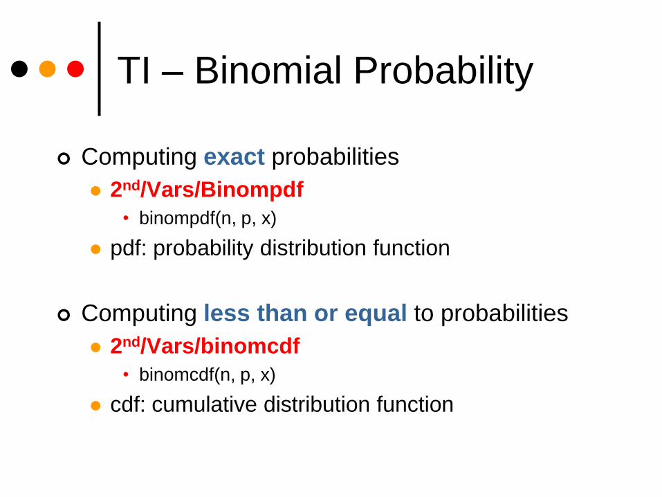
Computing exact probabilities
2nd/Vars/Binompdf
• binompdf(n, p, x)
pdf: probability distribution function
Computing less than or equal to probabilities
2nd/Vars/binomcdf
• binomcdf(n, p, x)
cdf: cumulative distribution function

Binomial Coefficient
There is a mathematical way to count the total number of
ways to arrange k out of n objects. This is called
“n choose k” or binomial coefficient.
!
! !n k
n nC
k k n k
n k
nC
k
and is called “n choose k” is given by the formula

Binomial Formula
n = number of trials
p = probability of success and q = 1 – p for failures
X = number of success in n trials
( ) k n k
n kP X k c p q
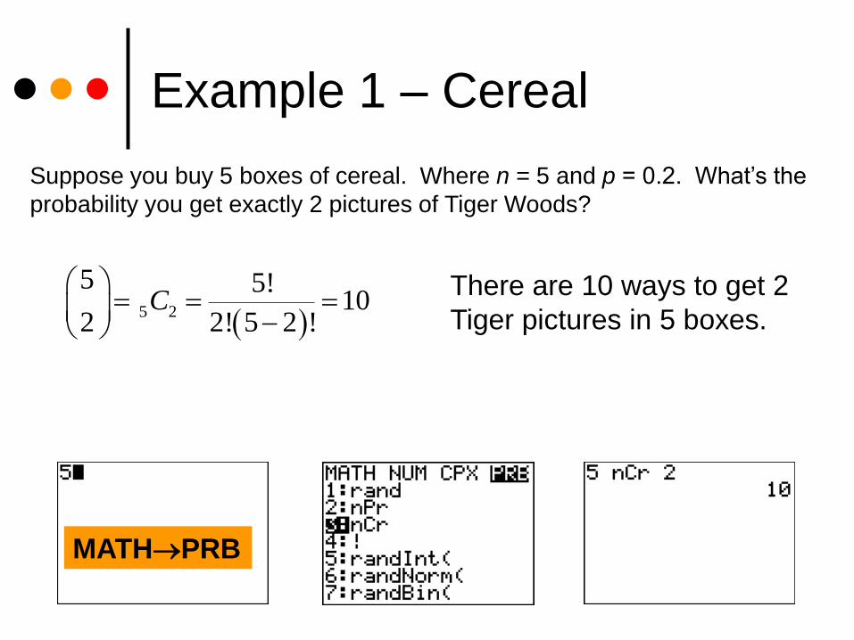
Example 1 – Cereal
Suppose you buy 5 boxes of cereal. Where n = 5 and p = 0.2. What’s the
probability you get exactly 2 pictures of Tiger Woods?
5 2
5 5!10
2 2! 5 2 !C
There are 10 ways to get 2
Tiger pictures in 5 boxes.
MATHPRB

Example 1 – Cereal
Suppose you buy 5 boxes of cereal. Where n = 5 and p = 0.2. What’s the
probability you get exactly 2 pictures of Tiger Woods?
2 3( 2) 10(0.20) (0.80) 0.2048P X
There are 10 ways to get 2 Tiger pictures in 5 boxes.
2nd Vars

Example – Cereal
The following table show the probability distribution function
(p.d.f) for the binomial random variable, X.
X = Tiger P(X)
0 0.32768
1 0.4096
2 0.2048
3 0.0512
4 0.0064
5 0.00032
5( 0) ( ) 0.80 0.32768
(5,0.20,0) 0.32768
(5,0.20,1) 0.4096
(5,0.20,2) 0.2048
(5,0.20,3) 0.0512
(5,0.20,4) 0.0064
(5,0.20,5) 0.00032
P X P FFFFF
Binompdf
Binompdf
Binompdf
Binompdf
Binompdf
Binompdf

Example – Cereal
The following table show the cumulative distribution function
(c.d.f) for the binomial random variable, X.
0 1 2 3 4 5
( ) 0.32768 0.4096 0.2048 .0512 .0064 .00032
( 0) ( 1) ( 2) ( 3) ( 4) ( 5)( )
0.32768 0.73728 0.94208 0.99328 0.99968 1
cdf
X
P X
P X P X P X P X P X P XP X
(5,0.20,0) 0.32768
(5,0.20,2) 0.73728
(5,0.20,3) 0.99328
Binomcdf
Binomcdf
Binomcdf
(5,0.20,4) 0.99968
(5,0.20,5) 1
Binomcdf
Binomcdf
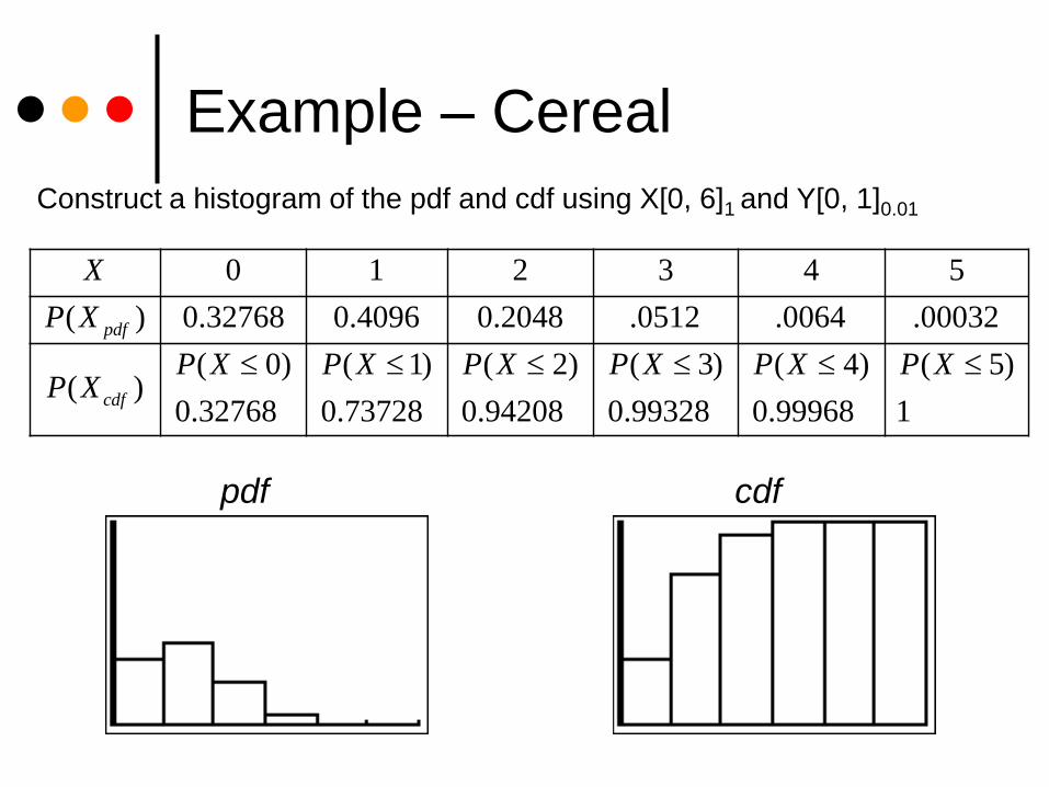
Example – Cereal
0 1 2 3 4 5
( ) 0.32768 0.4096 0.2048 .0512 .0064 .00032
( 0) ( 1) ( 2) ( 3) ( 4) ( 5)( )
0.32768 0.73728 0.94208 0.99328 0.99968 1
cdf
X
P X
P X P X P X P X P X P XP X
Construct a histogram of the pdf and cdf using X[0, 6]1 and Y[0, 1]0.01
pdf cdf

Example – Page 441, #8.2
In each of the following cases, decide whether or not
a binomial distribution is an appropriate model, and give
your reasons.
A). Fifty students are taught the about the binomial
distributions by a television program. After completing
their study, all students take the same examination.
The number who pass is counted.
Yes, it would be reasonable to assume that the results
for the 50 students are independent, and each has the same
chance of passing.

Example – Page 441, #8.2
B). A student studies binomial distributions using computer
instruction. After the initial instruction is completed, the
computer presents 10 problems. The student solves
each problem and enters the answer: the computer gives
additional instruction between problems if the student’s
answer is wrong. The number of problems that the
student solves correctly is counted.
No; since the student receives instruction after incorrect
answers, her probability of success is likely to increase.

Example – Page 441, #8.2
C). A chemist repeats a solubility test 10 times on the same
substance. Each test is conducted at temperature 10°
higher than the previous test. She counts the number of
times that the substance dissolves completely.
No; temperature may affect the outcome of the test.

Example – Page 445, #8.4
Suppose that James guesses on each question of a 50-item
true-false quiz. Find the probability that James passes if
A). a score of 25 or more correct is needed to pass.
X = the number of correct answers. X is binomial
with n = 50 and p = 0.50
( 25) ( 25) ( 26) ... ( 50) P X P X P X P X
1 (50,0.50,24)binomialcdf 0.556
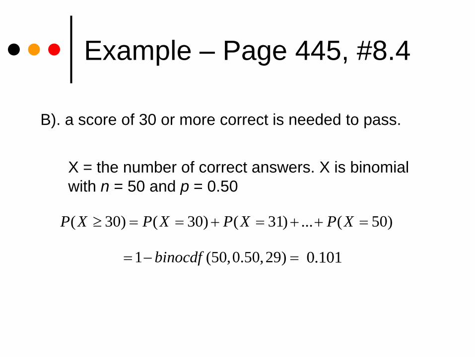
Example – Page 445, #8.4
B). a score of 30 or more correct is needed to pass.
X = the number of correct answers. X is binomial
with n = 50 and p = 0.50
( 30) ( 30) ( 31) ... ( 50) P X P X P X P X
1 (50,0.50,29) binocdf 0.101

Example – Page 445, #8.4
C). a score of 32 or more correct is needed to pass.
X = the number of correct answers. X is binomial
with n = 50 and p = 0.50
( 32) ( 32) ( 33) ... ( 50) P X P X P X P X
1 (50,0.50,31) binocdf 0.032
Example – Page 446, #8.6
According to a 2000 study by the Bureau of Justice Statistics, approximately
2% of the nation’s 72 million children had a parent behind bars – nearly 1.5
million minors. Let X be the number of children who had an incarcerated
parent. Suppose that 100 children are randomly selected.
A) Does X satisfy the requirements for a binomial setting?
Explain. If X = B(n, p), what are n and p?
Yes, if the 100 children are randomly selected, it is
extremely likely that the result for one child will not influence
the result for any other child. “Success” in this context
means having an incarcerated parent. Where n = 100 and
p = 0.02

Example – Page 446, #8.6
X = B(100, 0.02)
B). Describe P(X = 0) in words. Then find P(X = 0) and
P(X = 1).
P(X = 0) = the probability of none of the 100 selected
children having incarcerated parent.
( 0) (100,0.02,0) P X binompdf 0.133
( 1) (100,0.02,1) P X binompdf 0.271

Example – Page 446, #8.6
X = B(100, 0.02)
C). What is the probability that 2 or more of the 100 children
have a parent behind bars.
1 (100,0.02,1) 0.596 binomcdf
( 2) ( 2) ( 3) ... ( 100) P X P X P X P X
About 60% of the time we’ll find 2 or more children with
parents behind bars among the 100 children.

Example – Page 449, #8.10
Suppose you purchase a bundle of 10 bare-root broccoli plants. The
sales clerk tells you that on average you can expect 5% of the plants to
die before purchasing any broccoli. Assume that the bundle is a
random sample of plants. Use the binomial formula to find the
probability that you will lose at most one of the broccoli plants.
Let X = the number of broccoli plants that you lose
n = 10 and p = 0.05
( 1) ( 0) ( 1)P X P X P X
0 10 1 9
10 0 10 10.05 0.95 0.05 0.95
0.59874 0.31512 0.914
C C

Lesson 8-1, Part 2
Mean and Standard Deviation

Mean and
Standard Deviation
If X is binomial random variable with parameters n and p,
then the mean and standard deviation of X are:
(1 )
X
X
np
np p npq

Example – Page 454, #8.16
A) What is the mean number of Hispanics on randomly
chosen committees of 15 workers in Exercise 8.13
(page 449)?
15
0.3
n
p
15(0.3)
4.5
np
B) What is the standard deviation σ of the count X of
Hispanic members?
15(0.3)(0.7) 1.77482npq

Example – Page 454, #8.16
C) Suppose that 10% of the factory workers were Hispanic.
Then p = 0.1. What is σ in this case? What is σ if
p = 0.01? What does your work show about the behavior
of the standard deviation of binomial distribution as the
probability of a success gets closer to 0?
15
0.10
n
p
15(0.1)(0.9) 1.1619npq
15
.01
n
p
15(0.01)(0.99) 0.385357
As p gets closer to 0, σ gets closer to 0.

Approximate a Binomial Distribution
with a Normal Distribution if:
np 10
nq 10
then µ = np and = npq
and the random variable has
distribution.(normal)
a

Example – Page 455, #8.20
You operate a restaurant. You read that a sample survey by the
National Restaurant Association shows that 40% of adults are
committed to eating nutritious food when eating away from home. To
help plan your menu, you decide to conduct a sample survey in your
own area. You will use random digit dialing to contact an SRS of
200 households by telephone.
A). If the national results holds in area, it is reasonable to use the
binomial distribution with n = 200 and p = 0.4 to describe the count
X of respondents who seek nutritional food when eating out.
Explain why.
Yes, this study satisfies the requirements of a
binomial setting.

Example – Page 455, #8.20
B). What is the mean number of nutrition-conscious people in your
sample if p = 0.4 it true? What is the standard deviation?
200(0.4) 80np
200(.4)(.6) 48 6.9282npq
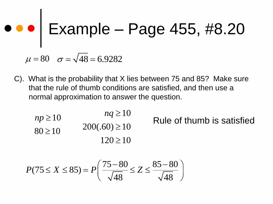
Example – Page 455, #8.20
80 48 6.9282
C). What is the probability that X lies between 75 and 85? Make sure
that the rule of thumb conditions are satisfied, and then use a
normal approximation to answer the question.
10
80 10
np
10
200(.60) 10
120 10
nq
Rule of thumb is satisfied
75 80 85 80(75 85)
48 48P X P Z

Example – Page 455, #8.20
80 48 6.9282
75 80 85 80(75 85)
48 48P X P Z
( 0.72 0.72)P Z
-0.72 0.720
( 0.72,0.72,0,1) 0.528475normalcdf
0.5285
(75,85,80, 48) 0.5295normalcdf

Lesson 8-2
Geometric Distributions
Example 2 – Cereal
Suppose a cereal manufacturer puts pictures of famous
athletes on cards in boxes of cereal, in the hope of
increasing sales. The manufacture announces that 20%
of the boxes contain a picture of Tiger Woods, 30% a
picture of Lance Armstrong, and the rest a picture of
Serena Williams.
You’ve got to have the Tiger Woods picture, so you start
madly opening boxes of cereal, hoping to find one.
Assuming that the pictures are randomly distributed,
there’s a 20% chance you succeed on any box you open.

Example 2 – Cereal
What’s the probability you find his picture in the first box of
cereal? It’s 20%, of course. We could write
P(# of boxes = 1) = 0.20.
How about the probability that you don’t find Tiger until
the second box? P(# of boxes = 2) = (0.8)(0.2) = 0.16
Of course, you could have a run of bad luck. Maybe
you won’t find Tiger until the fifth box of cereal. What
are the chances of that?
P(# of boxes = 5) = (0.80)4(0.20) = 0.08192

Geometric Distributions
Random variable X = the number of trials required to obtain the first success
X is a geometric random variable There are only two outcomes: success or failure.
The variable of interest is the number of trials required to obtain the first success
The n observations are independent.
The probability of success p is the same for each observation.
Since n is not fixed there could be an infinite number of X values
The probability histogram for a geometric is always skewed to the right.

Geometric Distributions
1 1( ) 1
n nP X n p p q p
The probability formula that X is equal to n is given by
the following formula:
The probability that X is greater than n is given by the
following formula:
( ) (1 )n nP X n p q

Mean and
Standard Deviation
The expected value of a geometric random variable is:
1
p
The standard deviation of geometric random variable is:
2
q
p
Example – Page 468, #38
An experiment consists of rolling a die until a prime number
(2, 3, or 5) is observed. Let X = number of rolls required to
get the first prime number.
A). Verify that X has a geometric distribution.
The four conditions of geometric setting hold, with
probability of success ½

Example – Page 468, #38
B). Construct probability distribution table to include at
least 5 entries for the probability of X. Record
probabilities to four decimal places.
geometpdf(0.50, L1)

Example – Page 468, #38
X 1 2 3 4 5
P(X) 0.50 0.25 0.125 0.0625 0.03125
c.d.f 0.50 0.75 0.875 0.9375 0.96875
geometcdf(0.50, L1)

Example – Page 468, #38
C). Construct a graph of the pdf of X.

Example – Page 468, #38
D). Compute the cdf of X and plot its histogram
Example – Page 474, #8.44
The State Department is trying to identify an individual who speaks Farsi
to fill a foreign embassy position. They have determine that 4% of the
applicants pool are fluent in Farsi.
A) If applicants are contacted randomly, how many
individuals can they expect to interview in order to
find one who is fluent in Farsi?
1 125
0.04p applicants

Example – Page 474, #8.44
B) What is the probability that they will have to interview
more than 25 until they find one who speaks Farsi? More
than 40?
25( 25) (1 ) (1 0.04) 0.3604nP x p
( 25) 1 ( 25) 1 (0.04,25) 0.3604P X P X geometcdf
( 40) 1 ( 40) 1 (0.04,40) 0.1954P X P X geometcdf


