CHAPTER 21 INTERFEROMETERS -...

CHAPTER 21 INTERFEROMETERS

P . Hariharan Di y ision of Applied Physics CSIRO Sydney , Australia

2 1 . 1 GLOSSARY

A area

C ratio of peaks to valleys

d thickness

F finesse

FSR free spectral range

I intensity

J i ( ) Bessel function

L fiber length

m integer

N number of fringes

p optical path dif ference

R reflectance

r radius

T transmittance

l s synthetic wavelength

θ angle

… frequency

f phase

2 1 . 2 INTRODUCTION

Optical interferometers have made feasible a variety of precision measurements using the interference phenomena produced by light waves . 1 , 2 After a brief survey of the basic types of interferometers , this article will describe some of the interferometers that can be used

21 .1

21 .2 OPTICAL INSTRUMENTS

for such applications as measurements of lengths and small changes in length ; optical testing ; studies of surface structure ; measurements of the pressure and temperature distribution in gas flows and plasmas ; measurements of particle velocities and vibration amplitudes ; rotating sensing ; measurements of temperature , pressure , and electric and magnetic fields ; wavelength measurements , and measurements of the angular diameter of stars , as well as , possibly , the detection of gravitational waves .

2 1 . 3 BASIC TYPES OF INTERFEROMETERS

Interferometric measurements require an optical arrangement in which two or more beams , derived from the same source but traveling along separate paths , are made to interfere . Interferometers can be classified as two - beam interferometers or multiple - beam interferometers according to the number of interfering beams ; they can also be grouped according to the methods used to obtain these beams . The most commonly used form of beam splitter is a partially reflecting metal or dielectric film on a transparent substrate ; other devices that can be used are polarizing prisms and dif fraction gratings . The best known types of two-beam interferometers are the Fizeau , the Michelson , the Mach- Zehnder , and the Sagnac interferometers ; the best known multiple-beam interferometer is the Fabry-Perot interferometer .

The Fizeau Interferometer

In the Fizeau interferometer , as shown in Fig . 1 , interference fringes of equal thickness are formed between two flat surfaces separated by an air gap and illuminated with a collimated beam . If one of the surfaces is a standard reference flat surface , the fringe pattern is a contour map of the errors of the test surface . Modified forms of the Fizeau interferometer are also used to test convex and concave surfaces by using a converging or diverging beam . 3

The Michelson Interferometer

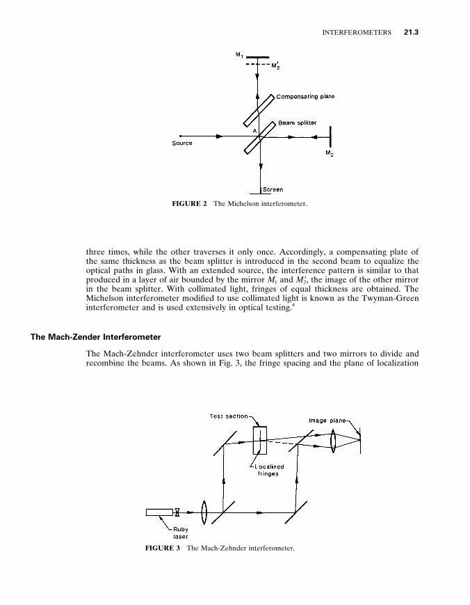
The Michelson interferometer , shown schematically in Fig . 2 , uses a beam splitter to divide and recombine the beams . As can be seen , one of the beams traverses the beam splitter

FIGURE 1 The Fizeau interferometer .

INTERFEROMETERS 21 .3

FIGURE 2 The Michelson interferometer .

three times , while the other traverses it only once . Accordingly , a compensating plate of the same thickness as the beam splitter is introduced in the second beam to equalize the optical paths in glass . With an extended source , the interference pattern is similar to that produced in a layer of air bounded by the mirror M 1 and M 9 2 , the image of the other mirror in the beam splitter . With collimated light , fringes of equal thickness are obtained . The Michelson interferometer modified to use collimated light is known as the Twyman-Green interferometer and is used extensively in optical testing . 4

The Mach-Zender Interferometer

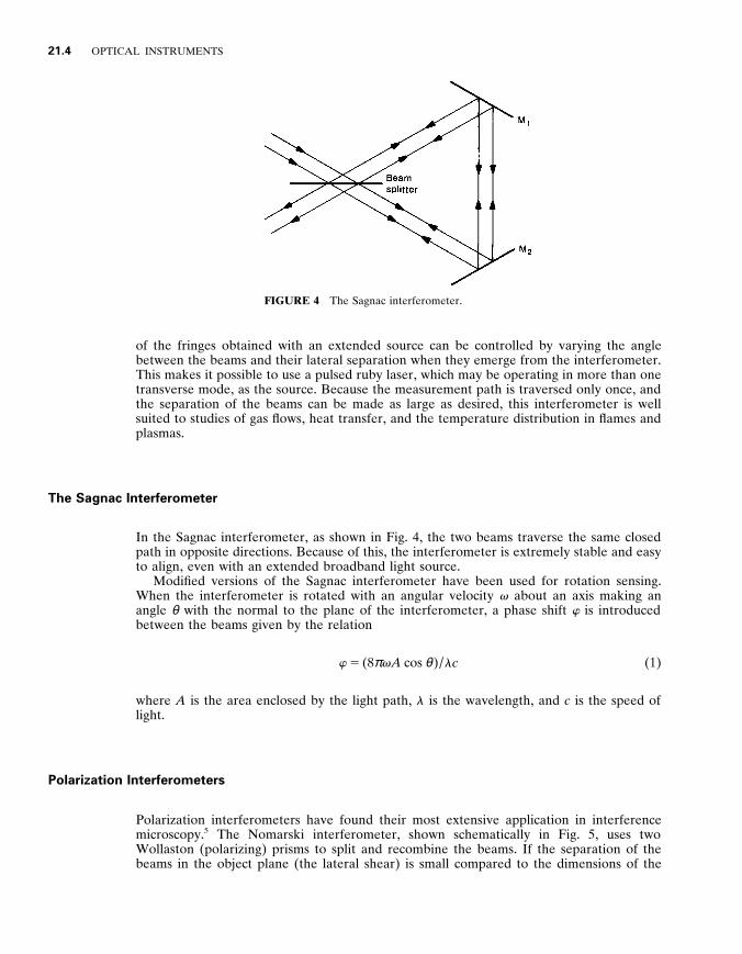
The Mach-Zehnder interferometer uses two beam splitters and two mirrors to divide and recombine the beams . As shown in Fig . 3 , the fringe spacing and the plane of localization

FIGURE 3 The Mach-Zehnder interferometer .


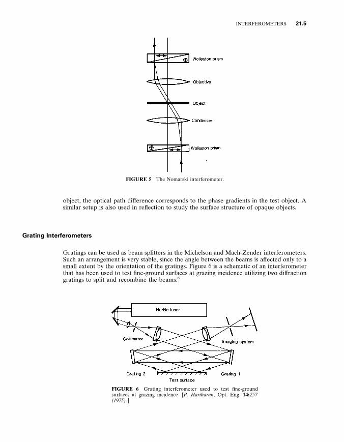
FIGURE 4 The Sagnac interferometer .

of the fringes obtained with an extended source can be controlled by varying the angle between the beams and their lateral separation when they emerge from the interferometer . This makes it possible to use a pulsed ruby laser , which may be operating in more than one transverse mode , as the source . Because the measurement path is traversed only once , and the separation of the beams can be made as large as desired , this interferometer is well suited to studies of gas flows , heat transfer , and the temperature distribution in flames and plasmas .

The Sagnac Interferometer

In the Sagnac interferometer , as shown in Fig . 4 , the two beams traverse the same closed path in opposite directions . Because of this , the interferometer is extremely stable and easy to align , even with an extended broadband light source .

Modified versions of the Sagnac interferometer have been used for rotation sensing . When the interferometer is rotated with an angular velocity v about an axis making an angle θ with the normal to the plane of the interferometer , a phase shift w is introduced between the beams given by the relation

w 5 (8 π v A cos θ ) / l c (1)

where A is the area enclosed by the light path , l is the wavelength , and c is the speed of light .

Polarization Interferometers

Polarization interferometers have found their most extensive application in interference microscopy . 5 The Nomarski interferometer , shown schematically in Fig . 5 , uses two Wollaston (polarizing) prisms to split and recombine the beams . If the separation of the beams in the object plane (the lateral shear) is small compared to the dimensions of the


FIGURE 5 The Nomarski interferometer .

object , the optical path dif ference corresponds to the phase gradients in the test object . A similar setup is also used in reflection to study the surface structure of opaque objects .

Grating Interferometers

Gratings can be used as beam splitters in the Michelson and Mach-Zender interferometers . Such an arrangement is very stable , since the angle between the beams is af fected only to a small extent by the orientation of the gratings . Figure 6 is a schematic of an interferometer that has been used to test fine-ground surfaces at grazing incidence utilizing two dif fraction gratings to split and recombine the beams . 6

FIGURE 6 Grating interferometer used to test fine-ground surfaces at grazing incidence . [ P . Hariharan , Opt . Eng . 14 : 2 5 7 ( 1 9 7 5 ) . ]


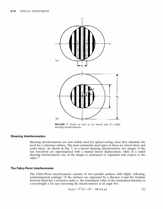
FIGURE 7 Fields of view in ( a ) lateral and ( b ) radial shearing interferometers .

Shearing Interferometers

Shearing interferometers are now widely used for optical testing , since they eliminate the need for a reference surface . The most commonly used types of shear are lateral shear and radial shear . As shown in Fig . 7 , in a lateral shearing interferometer two images of the test wavefront are superimposed with a mutual lateral displacement , while in a radial shearing interferometer one of the images is contracted or expanded with respect to the other . 7 , 8

The Fabry-Perot Interferometer

The Fabry-Perot interferometer consists of two parallel surfaces with highly reflecting , semitransparent coatings . 9 If the surfaces are separated by a distance d and the medium between them has a refractive index n , the normalized value of the transmitted intensity at a wavelength l for rays traversing the interferometer at an angle θ is

I T ( l ) 5 T 2 / (1 1 R 2 2 2 R cos w ) (2)


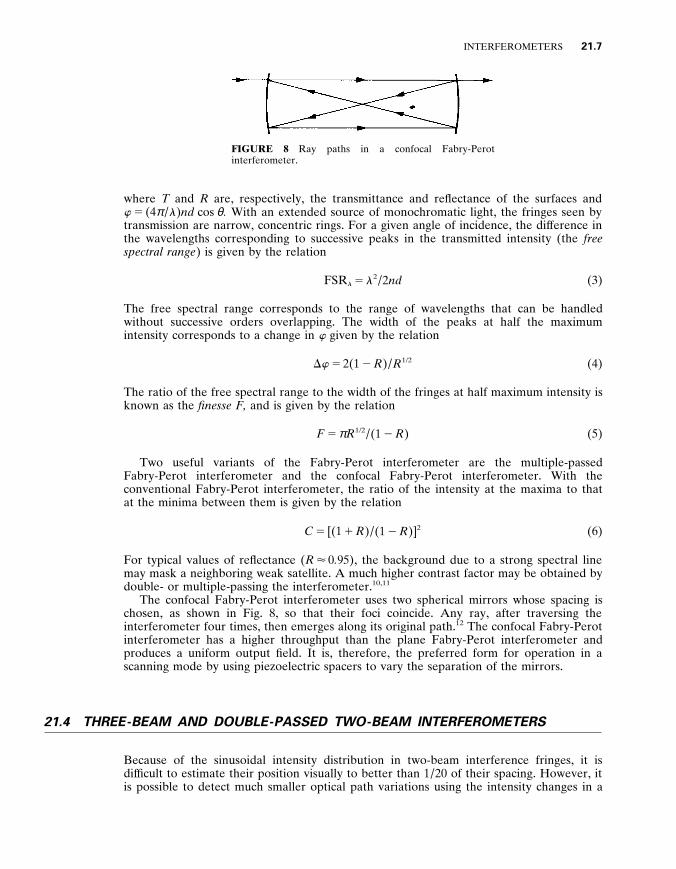
FIGURE 8 Ray paths in a confocal Fabry-Perot interferometer .

where T and R are , respectively , the transmittance and reflectance of the surfaces and w 5 (4 π / l ) nd cos θ . With an extended source of monochromatic light , the fringes seen by transmission are narrow , concentric rings . For a given angle of incidence , the dif ference in the wavelengths corresponding to successive peaks in the transmitted intensity (the free spectral range ) is given by the relation

FSR l 5 l 2 / 2 nd (3)

The free spectral range corresponds to the range of wavelengths that can be handled without successive orders overlapping . The width of the peaks at half the maximum intensity corresponds to a change in w given by the relation

D w 5 2(1 2 R ) / R 1 / 2 (4)

The ratio of the free spectral range to the width of the fringes at half maximum intensity is known as the finesse F , and is given by the relation

F 5 π R 1 / 2 / (1 2 R ) (5)

Two useful variants of the Fabry-Perot interferometer are the multiple-passed Fabry-Perot interferometer and the confocal Fabry-Perot interferometer . With the conventional Fabry-Perot interferometer , the ratio of the intensity at the maxima to that at the minima between them is given by the relation

C 5 [(1 1 R ) / (1 2 R )] 2 (6)

For typical values of reflectance ( R < 0 . 95) , the background due to a strong spectral line may mask a neighboring weak satellite . A much higher contrast factor may be obtained by double- or multiple-passing the interferometer . 1 0 , 1 1

The confocal Fabry-Perot interferometer uses two spherical mirrors whose spacing is chosen , as shown in Fig . 8 , so that their foci coincide . Any ray , after traversing the interferometer four times , then emerges along its original path . 1 2 The confocal Fabry-Perot interferometer has a higher throughput than the plane Fabry-Perot interferometer and produces a uniform output field . It is , therefore , the preferred form for operation in a scanning mode by using piezoelectric spacers to vary the separation of the mirrors .

2 1 . 4 THREE - BEAM AND DOUBLE - PASSED TWO - BEAM INTERFEROMETERS

Because of the sinusoidal intensity distribution in two-beam interference fringes , it is dif ficult to estimate their position visually to better than 1 / 20 of their spacing . However , it is possible to detect much smaller optical path variations using the intensity changes in a


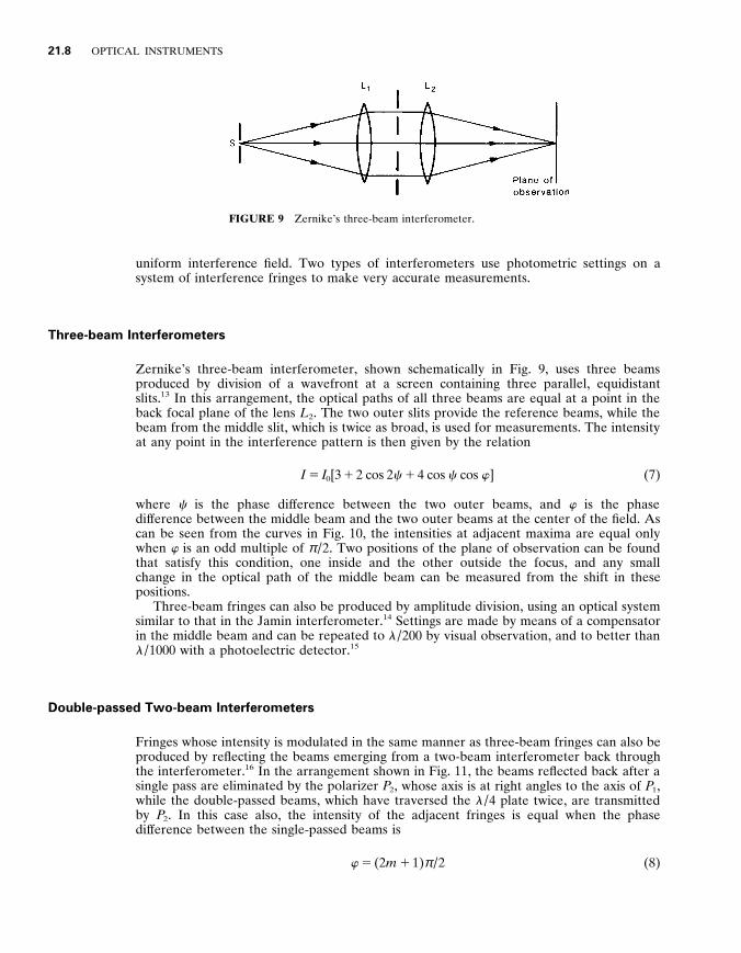
FIGURE 9 Zernike’s three-beam interferometer .

uniform interference field . Two types of interferometers use photometric settings on a system of interference fringes to make very accurate measurements .

Three-beam Interferometers

Zernike’s three-beam interferometer , shown schematically in Fig . 9 , uses three beams produced by division of a wavefront at a screen containing three parallel , equidistant slits . 1 3 In this arrangement , the optical paths of all three beams are equal at a point in the back focal plane of the lens L 2 . The two outer slits provide the reference beams , while the beam from the middle slit , which is twice as broad , is used for measurements . The intensity at any point in the interference pattern is then given by the relation

I 5 I 0 [3 1 2 cos 2 c 1 4 cos c cos w ] (7)

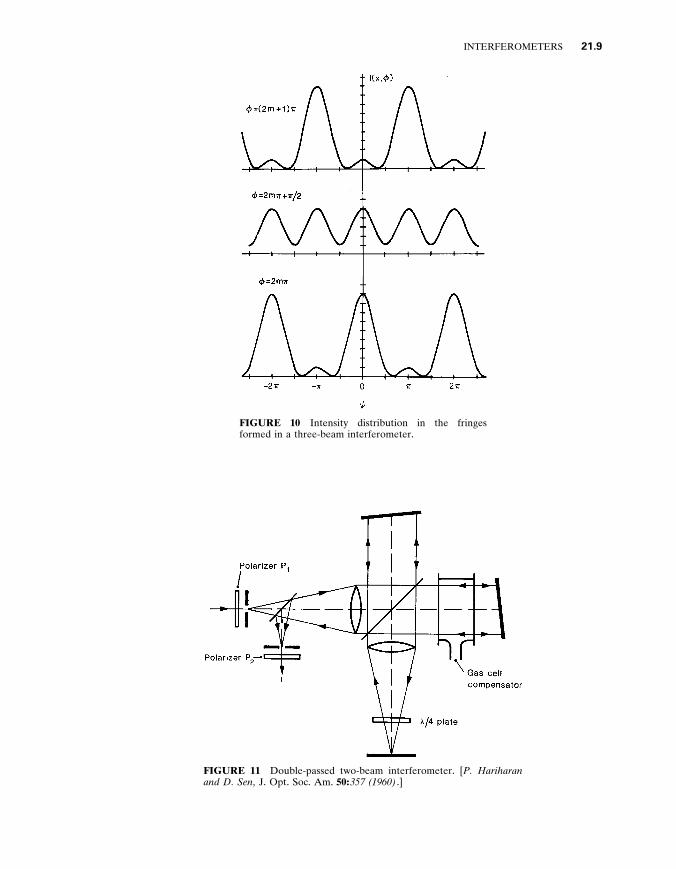
where c is the phase dif ference between the two outer beams , and w is the phase dif ference between the middle beam and the two outer beams at the center of the field . As can be seen from the curves in Fig . 10 , the intensities at adjacent maxima are equal only when w is an odd multiple of π / 2 . Two positions of the plane of observation can be found that satisfy this condition , one inside and the other outside the focus , and any small change in the optical path of the middle beam can be measured from the shift in these positions .

Three-beam fringes can also be produced by amplitude division , using an optical system similar to that in the Jamin interferometer . 1 4 Settings are made by means of a compensator in the middle beam and can be repeated to l / 200 by visual observation , and to better than l / 1000 with a photoelectric detector . 1 5

Double-passed Two-beam Interferometers

Fringes whose intensity is modulated in the same manner as three-beam fringes can also be produced by reflecting the beams emerging from a two-beam interferometer back through the interferometer . 1 6 In the arrangement shown in Fig . 11 , the beams reflected back after a single pass are eliminated by the polarizer P 2 , whose axis is at right angles to the axis of P 1 , while the double-passed beams , which have traversed the l / 4 plate twice , are transmitted by P 2 . In this case also , the intensity of the adjacent fringes is equal when the phase dif ference between the single-passed beams is

w 5 (2 m 1 1) π / 2 (8)


FIGURE 10 Intensity distribution in the fringes formed in a three-beam interferometer .

FIGURE 11 Double-passed two-beam interferometer . [ P . Hariharan and D . Sen , J . Opt . Soc . Am . 50 : 3 5 7 ( 1 9 6 0 ) . ]


where m is an integer . Measurements can be made with a precision of l / 1000 using a gas cell as a compensator .

2 1 . 5 FRINGE - COUNTING INTERFEROMETERS

One of the main applications of interferometry has been in accurate measurements of length using the wavelengths of stabilized lasers . Because of the high degree of coherence of laser light , interference fringes can be obtained even with quite large optical path dif ferences , and electronic fringe counting has become a very practical technique for length measurements .

The earliest fringe counting interferometers used an optical system giving two uniform interference fields , in one of which an additional phase dif ference of π / 2 was introduced between the interfering beams . Two photodetectors viewing these fields provided signals in quadrature that were used to drive a bidirectional counter . Another arrangement used two orthogonally polarized beams which were converted by a l / 4 plate oriented at 45 8 into right- and left-handed circularly polarized beams , respectively . When these two beams were superposed , they produced a linearly polarized beam whose plane of polarization rotated through 360 8 for a change in the optical path dif frence of two wavelengths (an optical screw) . Changes in the orientation of the plane of polarization and , hence , in the optical path dif ference were monitored by a polarizer controlled by a servo system . 1 7

The very narrow spectral line widths of lasers make it possible to use a heterodyne system , which has the advantage that its operation is not significantly af fected by variations in the intensity of the source . In one implementation of this technique , a He-Ne laser is forced to oscillate simultaneously at two frequencies , … 1 and … 2 , separated by a constant frequency dif ference of about 2 MHz , by applying an axial magnetic field . 1 8 These two waves , which are circularly polarized in opposite senses , are converted to orthogonal linear polarizations by a l / 4 plate . Alternatively , two acousto-optic modulators driven at dif ferent frequencies can be used to introduce a suitable frequency dif ference between two orthogonally polarized beams derived from a single-frequency laser .

As shown in Fig . 12 , a polarizing beam splitter reflects one beam to a fixed reflector , while the other is transmitted to a movable reflector . A dif ferential counter receives the

FIGURE 12 Heterodyne fringe-counting interferometer . [ After J . N . Dukes and G . B . Gordon , Hewlett-Packard Journal , 21 ( 1 2 ) ( 1 9 7 0 ) . ÷ Copyright Hewlett-Packard Company . Reproduced with permission . ]


beat frequencies from the photodetector D S and a reference photodetector D R . If the two reflectors are stationary , the two beat frequencies are the same , and the net count is zero . However , if one of the optical paths is varied by translating one of the reflectors , the change in wavelength is given by the net count .

2 1 . 6 TWO - WAVELENGTH INTERFEROMETRY

If a length is known within certain limits , the use of a wavelength longer than the separation of these limits permits its exact value to be determined unambiguously by a single interferometric measurement . One way to synthesize such a long wavelength is by illuminating the interferometer simultaneously with two wavelengths l 1 and l 2 . The envelope of the fringes then corresponds to the interference pattern that would be obtained with a synthetic wavelength

l s 5 l 1 l 2 / u l 1 2 l 2 u (9)

This technique can be implemented very ef fectively with a carbon dioxide laser , since it can operate at a number of wavelengths that are known very accurately , yielding a wide range of synthetic wavelengths . 1 9

Two-wavelength interferometry and fringe-counting can be combined to measure lengths up to 100 m by switching the laser rapidly between two wavelengths as one of the mirrors of a Twyman-Green interferometer is moved over the distance to be measured . The output signal from a photodetector is squared , low-pass filtered , and processed in a computer to yield the fringe count and the phase dif ference for the corresponding synthetic wavelength . 2 0

2 1 . 7 FREQUENCY - MODULATION INTERFEROMETERS

New interferometric techniques are possible with laser diodes which can be tuned electrically over a range of wavelengths . 2 1 One of these is frequency-modulation interferometry .

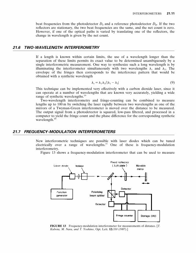
Figure 13 shows a frequency-modulation interferometer that can be used to measure

FIGURE 13 Frequency-modulation interferometer for measurements of distance . [ T . Kubota , M . Nara , and T . Yoshino , Opt . Lett . 12 : 3 1 0 ( 1 9 8 7 ) . ]


absolute distances , as well as relative displacements , with high accuracy . 2 2 In this arrangement , the signal beam reflected from the movable mirror returns as a circularly polarized beam , since it traverses the l / 8 plate twice . The reference beam reflected from the front surface of the l / 8 plate interferes with the two orthogonally polarized components of the signal beam at the two detectors to produce outputs that vary in quadrature and can be fed to a counter to determine the magnitude and sign of any displacement of the movable mirror .

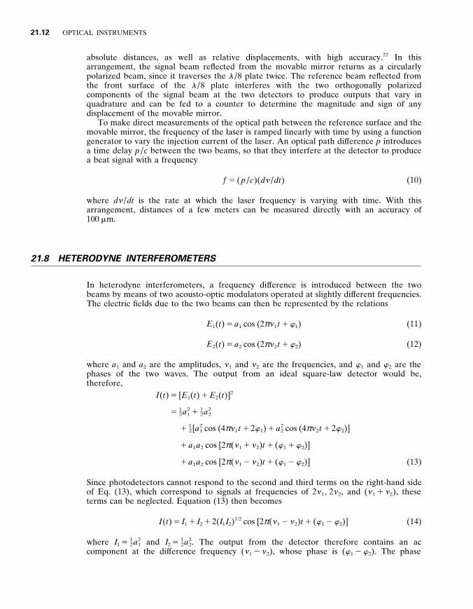
To make direct measurements of the optical path between the reference surface and the movable mirror , the frequency of the laser is ramped linearly with time by using a function generator to vary the injection current of the laser . An optical path dif ference p introduces a time delay p / c between the two beams , so that they interfere at the detector to produce a beat signal with a frequency

f 5 ( p / c )( d … / dt ) (10)

where d … / dt is the rate at which the laser frequency is varying with time . With this arrangement , distances of a few meters can be measured directly with an accuracy of 100 m m .

2 1 . 8 HETERODYNE INTERFEROMETERS

In heterodyne interferometers , a frequency dif ference is introduced between the two beams by means of two acousto-optic modulators operated at slightly dif ferent frequencies . The electric fields due to the two beams can then be represented by the relations

E 1 ( t ) 5 a 1 cos (2 π … 1 t 1 w 1 ) (11)

E 2 ( t ) 5 a 2 cos (2 π … 2 t 1 w 2 ) (12)

where a 1 and a 2 are the amplitudes , … 1 and … 2 are the frequencies , and w 1 and w 2 are the phases of the two waves . The output from an ideal square-law detector would be , therefore ,

I ( t ) 5 [ E 1 ( t ) 1 E 2 ( t )] 2

5 1 – 2 a 2 1 1 1 – 2 a 2

2

1 1 – 2 [ a 2 1 cos (4 π … 1 t 1 2 w 1 ) 1 a 2

2 cos (4 π … 2 t 1 2 w 2 )]

1 a 1 a 2 cos [2 π ( … 1 1 … 2 ) t 1 ( w 1 1 w 2 )]

1 a 1 a 2 cos [2 π ( … 1 2 … 2 ) t 1 ( w 1 2 w 2 )] (13)

Since photodetectors cannot respond to the second and third terms on the right-hand side of Eq . (13) , which correspond to signals at frequencies of 2 … 1 , 2 … 2 , and ( … 1 1 … 2 ) , these terms can be neglected . Equation (13) then becomes

I ( t ) 5 I 1 1 I 2 1 2( I 1 I 2 ) 1 / 2 cos [2 π ( … 1 2 … 2 ) t 1 ( w 1 2 w 2 )] (14)

where I 1 5 1 – 2 a 2 1 and I 2 5 1 – 2 a 2

2 . The output from the detector therefore contains an ac component at the dif ference frequency ( … 1 2 … 2 ) , whose phase is ( w 1 2 w 2 ) . The phase


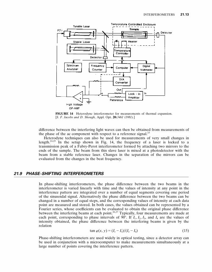
FIGURE 14 Heterodyne interferometer for measurements of thermal expansion . [ S . F . Jacobs and D . Shough , Appl . Opt . 20 : 3 4 6 1 ( 1 9 8 1 ) . ]

dif ference between the interfering light waves can then be obtained from measurements of the phase of the ac component with respect to a reference signal . 2 3

Heterodyne techniques can also be used for measurements of very small changes in length . 2 4 , 2 5 In the setup shown in Fig . 14 , the frequency of a laser is locked to a transmission peak of a Fabry-Perot interferometer formed by attaching two mirrors to the ends of the sample . The beam from this slave laser is mixed at a photodetector with the beam from a stable reference laser . Changes in the separation of the mirrors can be evaluated from the changes in the beat frequency .

2 1 . 9 PHASE - SHIFTING INTERFEROMETERS

In phase-shifting interferometers , the phase dif ference between the two beams in the interferometer is varied linearly with time and the values of intensity at any point in the interference pattern are integrated over a number of equal segments covering one period of the sinusoidal signal . Alternatively the phase dif ference between the two beams can be changed in a number of equal steps , and the corresponding values of intensity at each data point are measured and stored . In both cases , the values obtained can be represented by a Fourier series , whose coef ficients can be evaluated to obtain the original phase dif ference between the interfering beams at each point . 2 6 , 2 7 Typically , four measurements are made at each point , corresponding to phase intervals of 90 8 . If I 1 , I 2 , I 3 , and I 4 are the values of intensity obtained , the phase dif ference between the interfering beams is given by the relation

tan w ( x , y ) 5 ( I 1 2 I 3 ) / ( I 2 2 I 4 ) (15)

Phase-shifting interferometers are used widely in optical testing , since a detector array can be used in conjunction with a microcomputer to make measurements simultaneously at a large number of points covering the interference pattern .


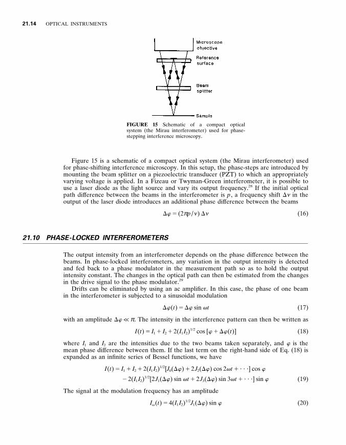
FIGURE 15 Schematic of a compact optical system (the Mirau interferometer) used for phase- stepping interference microscopy .

Figure 15 is a schematic of a compact optical system (the Mirau interferometer) used for phase-shifting interference microscopy . In this setup , the phase-steps are introduced by mounting the beam splitter on a piezoelectric transducer (PZT) to which an appropriately varying voltage is applied . In a Fizeau or Twyman-Green interferometer , it is possible to use a laser diode as the light source and vary its output frequency . 2 8 If the initial optical path dif ference between the beams in the interferometer is p , a frequency shift D … in the output of the laser diode introduces an additional phase dif ference between the beams

D w 5 (2 π p / … ) D … (16)

2 1 . 1 0 PHASE - LOCKED INTERFEROMETERS

The output intensity from an interferometer depends on the phase dif ference between the beams . In phase-locked interferometers , any variation in the output intensity is detected and fed back to a phase modulator in the measurement path so as to hold the output intensity constant . The changes in the optical path can then be estimated from the changes in the drive signal to the phase modulator . 2 9

Drifts can be eliminated by using an ac amplifier . In this case , the phase of one beam in the interferometer is subjected to a sinusoidal modulation

D w ( t ) 5 D w sin v t (17)

with an amplitude D w Ô π . The intensity in the interference pattern can then be written as

I ( t ) 5 I 1 1 I 2 1 2( I 1 I 2 ) 1 / 2 cos [ w 1 D w ( t )] (18)

where I 1 and I 2 are the intensities due to the two beams taken separately , and w is the mean phase dif ference between them . If the last term on the right-hand side of Eq . (18) is expanded as an infinite series of Bessel functions , we have

I ( t ) 5 I 1 1 I 2 1 2( I 1 I 2 ) 1 / 2 [ J 0 ( D w ) 1 2 J 2 ( D w ) cos 2 v t 1 ? ? ? ] cos w

2 2( I 1 I 2 ) 1 / 2 [2 J 1 ( D w ) sin v t 1 2 J 3 ( D w ) sin 3 v t 1 ? ? ? ] sin w (19)

The signal at the modulation frequency has an amplitude

I v ( t ) 5 4( I 1 I 2 ) 1 / 2 J 1 ( D w ) sin w (20)


FIGURE 16 Schematic of a phase-locked interferometer using a laser diode source . [ T . Suzuki , O . Sasaki , and T . Maruyama , Appl . Opt . 28 : 4 4 0 7 ( 1 9 8 9 ) . ]

and drops to zero when w 5 m π , where m is an integer . Since , at this point , both the magnitude and the sign of this signal change , it can be used as the input to a servo system that locks the phase dif ference between the beams at this point .

With a laser diode , it is possible to compensate for changes in the optical path dif ference by a change in the illuminating wavelength . A typical setup is shown in Fig . 16 . The injection current of the laser then consists of a dc bias current i 0 , a control current i c , and a sinusoidal modulation current i m ( t ) 5 i m cos v t whose amplitude is chosen to produce the required phase modulation . 3 0

Direct measurements of changes in the optical path are possible by sinusoidal phase-modulating interferometry , which uses a similar setup , except that in this case the amplitude of the phase modulation is much larger (typically around π radians) . The modulation amplitude is determined from the amplitudes of the components in the detector output corresponding to the modulation frequency and its third harmonic . The average phase dif ference between the beams can then be determined from the amplitudes of the components at the modulation frequency and its second harmonic . 3 1

2 1 . 1 1 LASER - DOPPLER INTERFEROMETERS

Light scattered from a moving particle undergoes a frequency shift , due to the Doppler ef fect , that is proportional to the component of its velocity in a direction determined by the directions of illumination and viewing . With laser light , this frequency shift can be evaluated by measuring the frequency of the beats produced by the scattered light and a reference beam . 3 2 Alternatively , it is possible to observe the beats produced by scattered light from two illuminating beams incident at dif ferent angles . 3 3

Laser-Doppler interferometry can be used for measurements of the velocity of moving material , 3 4 as well as for measurements , at a given point , of the instantaneous flow velocity of a moving fluid to which suitable tracer particles have been added . 3 5 A typical optical


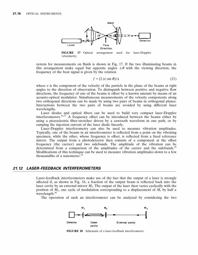
FIGURE 17 Optical arrangement used for laser-Doppler velocimetry .

system for measurements on fluids is shown in Fig . 17 . If the two illuminating beams in this arrangement make equal but opposite angles Ú θ with the viewing direction , the frequency of the beat signal is given by the relation

f 5 (2 u y u sin θ ) / l (21)

where y is the component of the velocity of the particle in the plane of the beams at right angles to the direction of observation . To distinguish between positive and negative flow directions , the frequency of one of the beams is of fset by a known amount by means of an acousto-optical modulator . Simultaneous measurements of the velocity components along two orthogonal directions can be made by using two pairs of beams in orthogonal planes . Interactions between the two pairs of beams are avoided by using dif ferent laser wavelengths .

Laser diodes and optical fibers can be used to build very compact laser-Doppler interferometers . 3 6 , 3 7 A frequency of fset can be introduced between the beams either by using a piezoelectric fiber-stretcher driven by a sawtooth waveform in one path , or by ramping the injection current of the laser diode linearly .

Laser-Doppler interferometry can also be used to measure vibration amplitudes . Typically , one of the beams in an interferometer is reflected from a point on the vibrating specimen , while the other , whose frequency is of fset , is reflected from a fixed reference mirror . The output from a photodetector then consists of a component at the of fset frequency (the carrier) and two sidebands . The amplitude of the vibration can be determined from a comparison of the amplitudes of the carrier and the sidebands . 3 8

Modifications of this technique can be used to measure vibration amplitudes down to a few thousandths of a nanometer . 3 9

2 1 . 1 2 LASER - FEEDBACK INTERFEROMETERS

Laser-feedback interferometers make use of the fact that the output of a laser is strongly af fected if , as shown in Fig . 18 , a fraction of the output beam is reflected back into the laser cavity by an external mirror M 3 . The output of the laser then varies cyclically with the position of M 3 , one cycle of modulation corresponding to a displacement of M 3 by half a wavelength . 4 0

The operation of such an interferometer can be analyzed by considering the two

FIGURE 18 Schematic of a laser-feedback interferometer .


mirrors M 3 and M 2 as a Fabry-Perot interferometer that replaces the output mirror of the laser . A variation in the spacing of M 3 and M 2 results in a variation in the reflectivity of this interferometer for the laser wavelength and , hence , in the gain of the laser .

A very compact laser-feedback interferometer can be set up with a single-mode laser diode . 4 1 Small displacements can be detected by measuring the changes in the laser output when the laser current is held constant . Measurements can be made over a larger range by mounting the laser on a piezoelectric transducer and using an active feedback loop to stabilize the length of the optical path from the laser to the mirror . 4 2

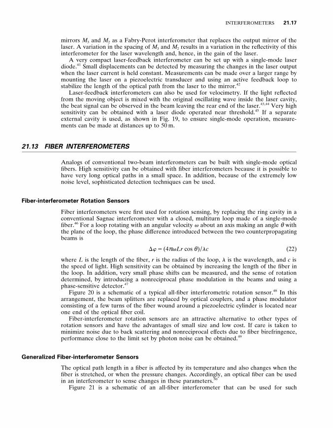
Laser-feedback interferometers can also be used for velocimetry . If the light reflected from the moving object is mixed with the original oscillating wave inside the laser cavity , the beat signal can be observed in the beam leaving the rear end of the laser . 43 , 44 Very high sensitivity can be obtained with a laser diode operated near threshold . 4 5 If a separate external cavity is used , as shown in Fig . 19 , to ensure single-mode operation , measurements can be made at distances up to 50 m .

2 1 . 1 3 FIBER INTERFEROMETERS

Analogs of conventional two-beam interferometers can be built with single-mode optical fibers . High sensitivity can be obtained with fiber interferometers because it is possible to have very long optical paths in a small space . In addition , because of the extremely low noise level , sophisticated detection techniques can be used .

Fiber-interferometer Rotation Sensors

Fiber interferometers were first used for rotation sensing , by replacing the ring cavity in a conventional Sagnac interferometer with a closed , multiturn loop made of a single-mode fiber . 4 6 For a loop rotating with an angular velocity v about an axis making an angle θ with the plane of the loop , the phase dif ference introduced between the two counterpropagating beams is

D w 5 (4 π v Lr cos θ ) / l c (22)

where L is the length of the fiber , r is the radius of the loop , l is the wavelength , and c is the speed of light . High sensitivity can be obtained by increasing the length of the fiber in the loop . In addition , very small phase shifts can be measured , and the sense of rotation determined , by introducing a nonreciprocal phase modulation in the beams and using a phase-sensitive detector . 4 7

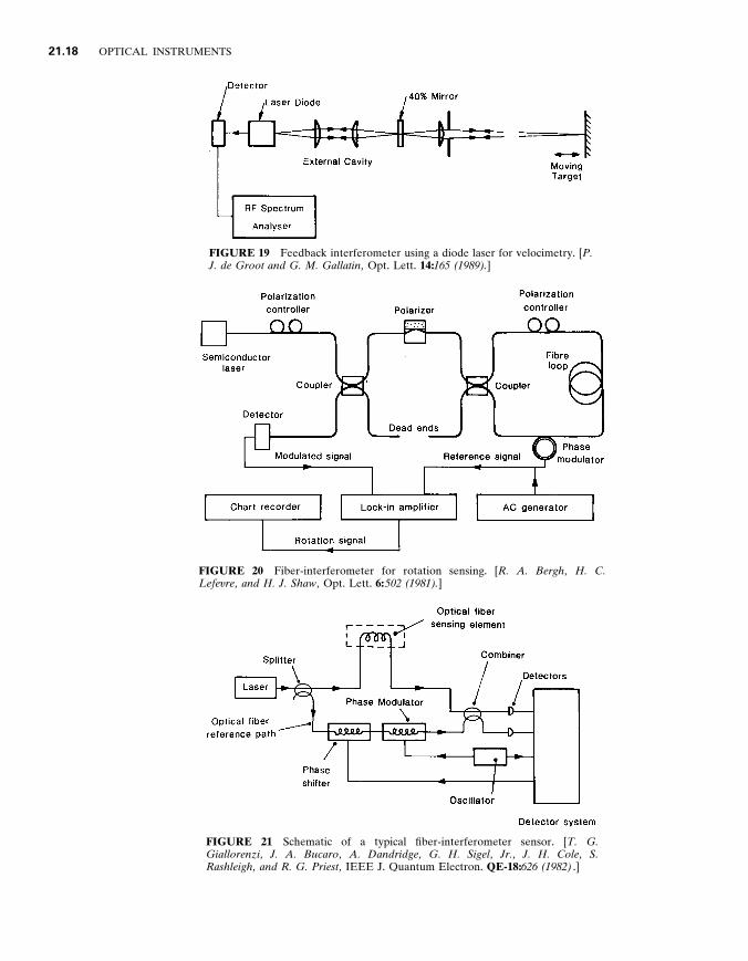
Figure 20 is a schematic of a typical all-fiber interferometric rotation sensor . 4 8 In this arrangement , the beam splitters are replaced by optical couplers , and a phase modulator consisting of a few turns of the fiber wound around a piezoelectric cylinder is located near one end of the optical fiber coil .

Fiber-interferometer rotation sensors are an attractive alternative to other types of rotation sensors and have the advantages of small size and low cost . If care is taken to minimize noise due to back scattering and nonreciprocal ef fects due to fiber birefringence , performance close to the limit set by photon noise can be obtained . 4 9

Generalized Fiber-interferometer Sensors

The optical path length in a fiber is af fected by its temperature and also changes when the fiber is stretched , or when the pressure changes . Accordingly , an optical fiber can be used in an interferometer to sense changes in these parameters . 5 0

Figure 21 is a schematic of an all-fiber interferometer that can be used for such


FIGURE 19 Feedback interferometer using a diode laser for velocimetry . [ P . J . de Groot and G . M . Gallatin , Opt . Lett . 14 : 1 6 5 ( 1 9 8 9 ) . ]

FIGURE 20 Fiber-interferometer for rotation sensing . [ R . A . Bergh , H . C . Lefe y re , and H . J . Shaw , Opt . Lett . 6 : 5 0 2 ( 1 9 8 1 ) . ]

FIGURE 21 Schematic of a typical fiber-interferometer sensor . [ T . G . Giallorenzi , J . A . Bucaro , A . Dandridge , G . H . Sigel , Jr . , J . H . Cole , S . Rashleigh , and R . G . Priest , IEEE J . Quantum Electron . QE-18 : 6 2 6 ( 1 9 8 2 ) . ]


measurements . 5 1 A layout analogous to a Mach-Zehnder interferometer has the advantage that it avoids optical feedback to the laser . Optical fiber couplers are used to divide and recombine the beams , and measurements can be made with either a heterodyne system or a phase-tracking system . Detection schemes involving either laser-frequency switching or a modulated laser source can also be used . Optical phase shifts as small as 10 2 6 radian can be detected .

Fiber interferometers have been used as sensors for mechanical strains and changes in temperature and pressure . They can be used for measurements of magnetic fields by bonding the fiber sensor to a magnetostrictive element . 5 2 Electric fields can also be measured by using a single-mode fiber sensor bounded to a piezoelectric film , or jacketed with a piezoelectric polymer . 5 3

Multiplexed Fiber-interferometer Sensors

Fiber-interferometer sensors can be multiplexed to measure dif ferent quantities at dif ferent locations with a single light source and detector and the same set of transmission lines . Techniques developed for this purpose include frequency-division multiplexing , time- division multiplexing , and coherence multiplexing . 54–57 These techniques can be combined to handle a larger number of sensors . 5 8

2 1 . 1 4 INTERFEROMETRIC WAVE METERS

The availability of tunable lasers has created a need for instruments that can measure their output wavelength with an accuracy commensurate with their narrow line width . Two types of interferometric wave meters have been developed for this purpose : dynamic wave meters and static wave meters . In dynamic wave meters , the measurement involves the movement of some element ; they have greater accuracy but can be used only with continuous sources . Static wave meters can also be used with pulsed lasers .

Dynamic Wave Meters

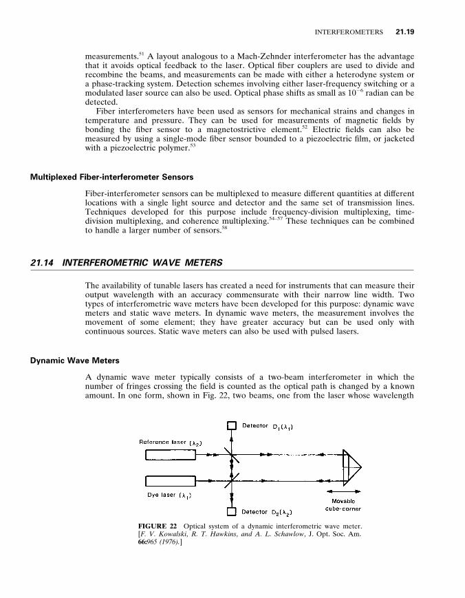
A dynamic wave meter typically consists of a two-beam interferometer in which the number of fringes crossing the field is counted as the optical path is changed by a known amount . In one form , shown in Fig . 22 , two beams , one from the laser whose wavelength

FIGURE 22 Optical system of a dynamic interferometric wave meter . [ F . V . Kowalski , R . T . Hawkins , and A . L . Schawlow , J . Opt . Soc . Am . 66 : 9 6 5 ( 1 9 7 6 ) . ]


is to be determined and another from a frequency stabilized He-Ne laser , traverse the same two paths in opposite directions . 5 9 The fringe system formed by these two lasers are imaged on the two detectors D 1 and D 2 , respectively . If , then , the end reflector is moved through a distance d , we have

l 1 / l 2 5 N 2 / N 1 (23)

where N 1 and N 2 are the numbers of fringes seen by D 1 and D 2 , respectively , and l 1 and l 2 are the wavelengths in air . To obtain the highest precision , it is also necessary to measure the fractional order numbers . This can be done by phase-locking an oscillator to an exact multiple of the frequency of the ac signal from the reference channel , or by digitally averaging the two signal frequencies . 6 0 It is also possible to use a vernier method in which the counting cycle starts and stops when the phases of the two signals coincide . 6 1 With these techniques , a precision of 1 part in 10 9 can be obtained .

Another type of dynamic wave meter uses a scanning Fabry-Perot interferometer in which the separation of the mirrors is changed slowly . If this interferometer is illuminated with the two wavelengths to be compared , peak transmission will be obtained for both wavelengths at intervals given by the condition

m 1 l 1 5 m 2 l 2 5 p (24)

where m 1 and m 2 are the changes in the integer order and p is the change in the optical path dif ference . 6 2 A precision of 1 part in 10 7 can be obtained with a range of movement of only 25 mm , because the Fabry-Perot fringes are much sharper than two-beam fringes .

Static Wave Meters

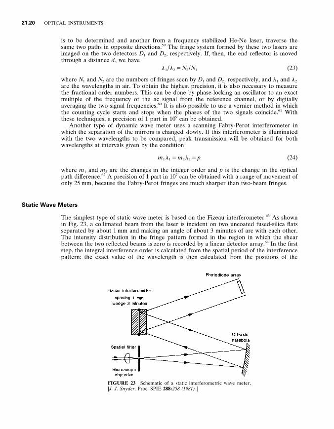
The simplest type of static wave meter is based on the Fizeau interferometer . 6 3 As shown in Fig . 23 , a collimated beam from the laser is incident on two uncoated fused-silica flats separated by about 1 mm and making an angle of about 3 minutes of arc with each other . The intensity distribution in the fringe pattern formed in the region in which the shear between the two reflected beams is zero is recorded by a linear detector array . 6 4 In the first step , the integral interference order is calculated from the spatial period of the interference pattern : the exact value of the wavelength is then calculated from the positions of the

FIGURE 23 Schematic of a static interferometric wave meter . [ J . J . Snyder , Proc . SPIE 288 : 2 5 8 ( 1 9 8 1 ) . ]


maxima and minima . This wave meter can be used with pulsed lasers , and up to 15 measurements can be made every second , with an accuracy of 1 part in 10 7 .

2 1 . 1 5 SECOND - HARMONIC AND PHASE - CONJUGATE INTERFEROMETERS

Nonlinear optical elements are used in second-harmonic and phase-conjugate interferometers . 6 5

Second-harmonic Interferometers

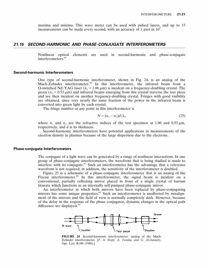
One type of second-harmonic interferometer , shown in Fig . 24 , is an analog of the Mach-Zehnder interferometer . 6 6 In this interferometer , the infrared beam from a Q-switched Nd : YAG laser ( l 1 5 1 . 06 m m) is incident on a frequency-doubling crystal . The green ( l 2 5 0 . 53 m m) and infrared beams emerging from this crystal traverse the test piece and are then incident on another frequency-doubling crystal . Fringes with good visibility are obtained , since very nearly the same fraction of the power in the infrared beam is converted into green light by each crystal .

The fringe number at any point in this interferometer is

N 5 ( n 1 2 n 2 ) d / l 2 (25)

where n 1 and n 2 are the refractive indices of the test specimen at 1 . 06 and 0 . 53 m m , respectively , and d is its thickness .

Second-harmonic interferometers have potential applications in measurements of the electron density in plasmas because of the large dispersion due to the electrons .

Phase-conjugate Interferometers

The conjugate of a light wave can be generated by a range of nonlinear interactions . In one group of phase-conjugate interferometers , the wavefront that is being studied is made to interfere with its conjugate . 6 7 Such an interferometer has the advantage that a reference wavefront is not required ; in addition , the sensitivity of the interferometer is doubled .

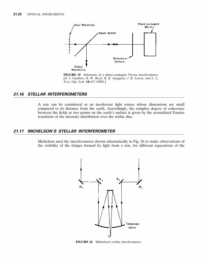
Figure 25 is a schematic of a phase-conjugate interferometer that is an analog of the Fizeau interferometer . 6 8 In this interferometer , the signal beam is incident on a conventional , partially reflecting mirror placed in front of a single crystal of barium titanate which functions as an internally self-pumped phase-conjugate mirror .

An interferometer in which both mirrors have been replaced by phase-conjugating mirrors has some unique properties . 6 9 Such an interferometer is unaf fected by misalign- ment of the mirrors and the field of view is normally completely dark . However , because of the delay in the response of the phase conjugator , dynamic changes in the optical path dif ference are displayed . 7 0

FIGURE 24 Second-harmonic interferometer : analog of the Mach- Zehnder interferometer . [ F . A . Hopf , A . Tomita , and G . Al - Jumaily , Opt . Lett . 5 : 3 8 6 ( 1 9 8 0 ) . ]


FIGURE 25 Schematic of a phase-conjugate Fizeau interferometer . [ D . J . Gauthier , R . W . Boyd , R . K . Jungquist , J . B . Lisson , and L . L . Voci , Opt . Lett . 14 : 3 2 3 ( 1 9 8 9 ) . ]

2 1 . 1 6 STELLAR INTERFEROMETERS

A star can be considered as an incoherent light source whose dimensions are small compared to its distance from the earth . Accordingly , the complex degree of coherence between the fields at two points on the earth’s surface is given by the normalized Fourier transform of the intensity distribution over the stellar disc .

2 1 . 1 7 MICHELSON ’ S STELLAR INTERFEROMETER

Michelson used the interferometer shown schematically in Fig . 26 to make observations of the visibility of the fringes formed by light from a star , for dif ferent separations of the

FIGURE 26 Michelson’s stellar interferometer .


mirrors . The separation at which the fringes disappeared was used to determine the angular diameter of the star . The problems encountered by Michelson in making measurements at mirror separations greater than 6 m have been overcome in a new version of this interferometer using modern detection , control , and data-processing techniques , that is expected to make measurements over baselines extending up to 1000 m . 7 1

The Intensity Interferometer

The intensity interferometer uses measurements of the degree of correlation between the fluctuations in the intensity at two photodetectors separated by a suitable distance . 7 2 With a thermal source , the correlation is proportional to the square of the modulus of the degree of coherence of the fields . The intensity interferometer has the advantage that atmospheric turbulence only af fects the phase of the incident wave and has no ef fect on the measured correlation . In addition , since the spectral bandwidth is limited by the electronics , it is only necessary to equalize the optical paths to within a few centimeters . It was therefore possible to use light collectors with a diameter of 6 . 5 m separated by distances up to 188 m , corresponding to a resolution of 0 . 42 3 10 2 3 second of arc .

Heterodyne Stellar Interferometers

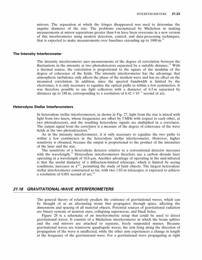
In heterodyne stellar interferometers , as shown in Fig . 27 , light from the star is mixed with light from two lasers , whose frequencies are of fset by 5 MHz with respect to each other , at two photodetectors , and the resulting heterodyne signals are multiplied in a correlator . The output signal from the correlator is a measure of the degree of coherence of the wave fields at the two photodetectors . 7 3

As in the intensity interferometer , it is only necessary to equalize the two paths to within a few centimeters in the heterodyne stellar interferometer . However , higher sensitivity is obtained , because the output is proportional to the product of the intensities of the laser and the star .

The sensitivity of a heterodyne detector relative to a conventional detector increases with the wavelength . 7 3 Heterodyne interferometers therefore use a carbon dioxide laser operating at a wavelength of 10 . 6 m m . Another advantage of operating in the mid-infrared is that the useful diameter of a dif fraction-limited telescope , which is limited by seeing conditions , increases as l 6 / 5 , permitting the study of faint objects . The largest heterodyne stellar interferometer constructed so far , with two 1 . 65-m telescopes , is expected to achieve a resolution of 0 . 001 second of arc . 7 4

2 1 . 1 8 GRAVITATIONAL - WAVE INTERFEROMETERS

The general theory of relatively predicts the existence of gravitational waves , which can be thought of as an alternating strain that propagates through space , af fecting the dimensions and spacing of all material objects . Potential sources of gravitational radiation are binary systems of neutron stars , collapsing supernovas , and black holes .

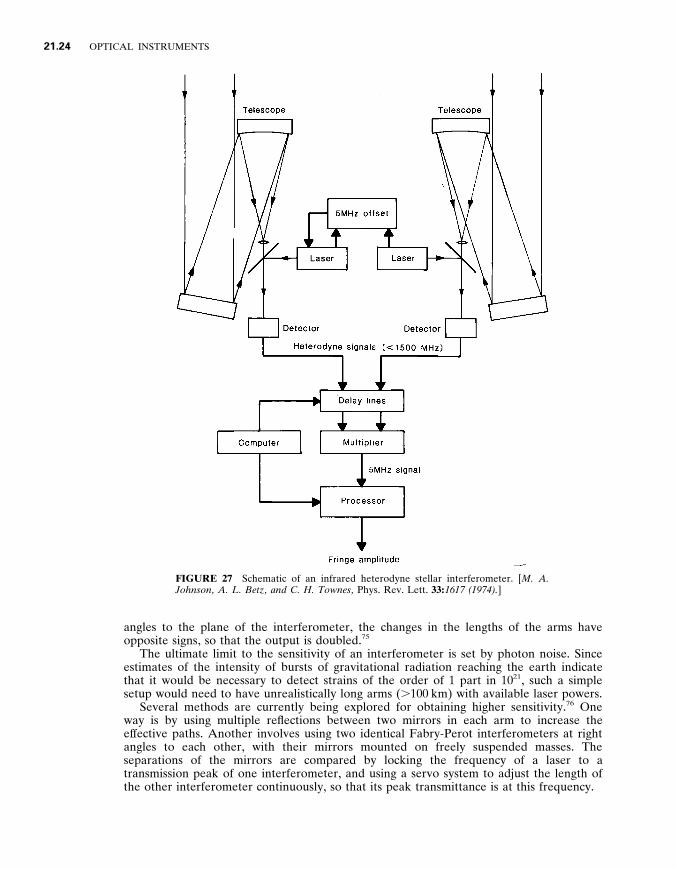
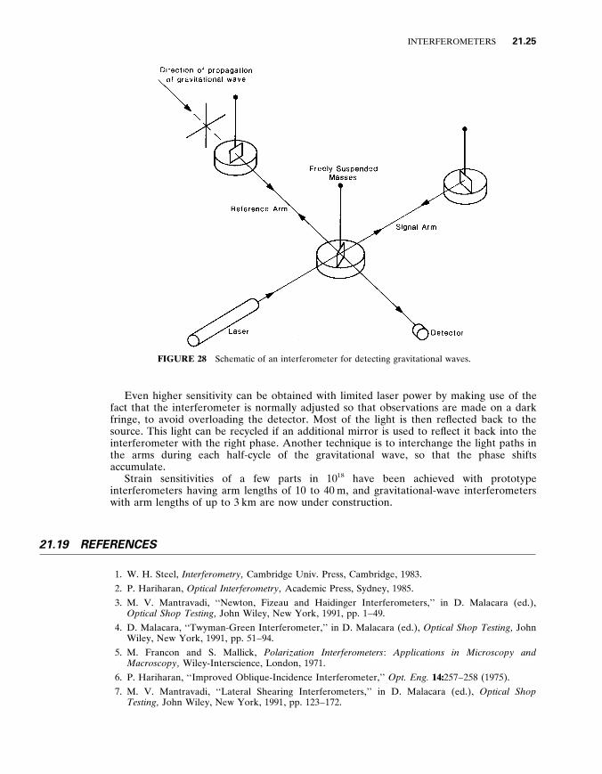
Figure 28 is a schematic of an interferometric setup that could be used to detect gravitational waves . It consists of a Michelson interferometer in which the beam splitter and the end mirrors are attached to separate , freely suspended masses . Because gravitational waves are transverse quadrupole waves , the arm lying along the direction of propagation of the wave is unaf fected , while the other arm experiences a change in length at the frequency of the gravitational wave . For a gravitational wave propagating at right


FIGURE 27 Schematic of an infrared heterodyne stellar interferometer . [ M . A . Johnson , A . L . Betz , and C . H . Townes , Phys . Rev . Lett . 33 : 1 6 1 7 ( 1 9 7 4 ) . ]

angles to the plane of the interferometer , the changes in the lengths of the arms have opposite signs , so that the output is doubled . 7 5

The ultimate limit to the sensitivity of an interferometer is set by photon noise . Since estimates of the intensity of bursts of gravitational radiation reaching the earth indicate that it would be necessary to detect strains of the order of 1 part in 10 2 1 , such a simple setup would need to have unrealistically long arms ( . 100 km) with available laser powers .

Several methods are currently being explored for obtaining higher sensitivity . 7 6 One way is by using multiple reflections between two mirrors in each arm to increase the ef fective paths . Another involves using two identical Fabry-Perot interferometers at right angles to each other , with their mirrors mounted on freely suspended masses . The separations of the mirrors are compared by locking the frequency of a laser to a transmission peak of one interferometer , and using a servo system to adjust the length of the other interferometer continuously , so that its peak transmittance is at this frequency .


FIGURE 28 Schematic of an interferometer for detecting gravitational waves .

Even higher sensitivity can be obtained with limited laser power by making use of the fact that the interferometer is normally adjusted so that observations are made on a dark fringe , to avoid overloading the detector . Most of the light is then reflected back to the source . This light can be recycled if an additional mirror is used to reflect it back into the interferometer with the right phase . Another technique is to interchange the light paths in the arms during each half-cycle of the gravitational wave , so that the phase shifts accumulate .

Strain sensitivities of a few parts in 10 1 8 have been achieved with prototype interferometers having arm lengths of 10 to 40 m , and gravitational-wave interferometers with arm lengths of up to 3 km are now under construction .

2 1 . 1 9 REFERENCES

1 . W . H . Steel , Interferometry , Cambridge Univ . Press , Cambridge , 1983 . 2 . P . Hariharan , Optical Interferometry , Academic Press , Sydney , 1985 . 3 . M . V . Mantravadi , ‘‘Newton , Fizeau and Haidinger Interferometers , ’’ in D . Malacara (ed . ) ,

Optical Shop Testing , John Wiley , New York , 1991 , pp . 1 – 49 . 4 . D . Malacara , ‘‘Twyman-Green Interferometer , ’’ in D . Malacara (ed . ) , Optical Shop Testing , John

Wiley , New York , 1991 , pp . 51 – 94 . 5 . M . Francon and S . Mallick , Polarization Interferometers : Applications in Microscopy and

Macroscopy , Wiley-Interscience , London , 1971 . 6 . P . Hariharan , ‘‘Improved Oblique-Incidence Interferometer , ’’ Opt . Eng . 14 : 257 – 258 (1975) . 7 . M . V . Mantravadi , ‘‘Lateral Shearing Interferometers , ’’ in D . Malacara (ed . ) , Optical Shop

Testing , John Wiley , New York , 1991 , pp . 123 – 172 .


8 . D . Malacara , ‘‘Radial , Rotational and Reversal Shear Interferometers , ’’ in D . Malacara (ed . ) , Optical Shop Testing , John Wiley , New York , 1991 , pp . 173 – 206 .

9 . J . M . Vaughan , The Fabry - Perot Interferometer , Adam Hilger , Bristol , 1989 . 10 . P . Hariharan and D . Sen , ‘‘Double-Passed Fabry – Perot Interferometer , ’’ J . Opt . Soc . Am .

51 : 398 – 399 (1961) . 11 . J . R . Sandercock , ‘‘Brillouin Scattering Study of SbSI Using a Double-Passed Stabilised Scanning

Interferometer , ’’ Opt . Commun . 2 : 73 – 76 (1970) . 12 . M . Hercher , ‘‘The Spherical Mirror Fabry-Perot Interferometer , ’’ Appl . Opt . 7 : 951 – 966 (1968) . 13 . F . Zernike , ‘‘A Precision Method for Measuring Small Phase Dif ferences , ’’ J . Opt . Soc . Am .

40 : 326 – 328 (1950) . 14 . P . Hariharan and D . Sen , ‘‘Three-Beam Interferometer , ’’ J . Sci . Instrum . 36 : 70 – 72 (1959) . 15 . P . Hariharan , D . Sen , and M . S . Bhalla , ‘‘Photoelectric Setting Methods for a Three-Beam

Interferometer , ’’ J . Sci . Instrum . 36 : 72 – 75 (1959) . 16 . P . Hariharan and D . Sen , ‘‘Double-Passed Two-Beam Interferometers , ’’ J . Opt . Soc . Am .

50 : 357 – 361 (1960) . 17 . G . R . Hopkinson , ‘‘The Optical Screw as a Path Dif ference Measurement and Control Device :

Analysis of Periodic Errors , ’’ J . Optics (Paris) 9 : 151 – 155 (1978) . 18 . J . N . Dukes and G . B . Gordon , ‘’A Two-Hundred Foot Yardstick With Graduations Every

Microinch , ’’ Hewlett - Packard Journal 21 (12) : 2 – 8 (1970) . 19 . C . W . Gillard and N . E . Buholz , ‘‘Progress in Absolute Distance Interferometry , ’’ Opt . Eng .

22 : 348 – 353 (1983) . 20 . H . Matsumoto , ‘‘Synthetic Interferometric Distance-Measuring System Using a CO 2 Laser , ’’

Appl . Opt . 25 : 493 – 498 (1986) . 21 . P . Hariharan , ‘‘Interferometry with Laser Diodes , ’’ Proc . SPIE 1400 : 2 – 10 (1991) . 22 . T . Kubota , M . Nara , and T . Yoshino , ‘‘Interferometer for Measuring Displacement and

Distance , ’’ Opt . Lett . 12 : 310 – 312 (1987) . 23 . R . Crane , ‘‘Interference Phase Measurement , ’’ Appl . Opt . 8 : 538 – 542 (1969) . 24 . S . F . Jacobs and D . Shough , ‘‘Thermal Expansion Uniformity of Heraeus-Amersil TO8E Fused

Silica , ’’ Appl . Opt . 20 : 3461 – 3463 (1981) . 25 . S . F . Jacobs , D . Shough , and C . Connors , ‘‘Thermal Expansion Uniformity of Materials for Large

Telescope Mirrors , ’’ Appl . Opt . 23 : 4237 – 4244 (1984) . 26 . J . H . Bruning , D . R . Herriott , J . E . Gallagher , D . P . Rosenfeld , A . D . White , and D . J .

Brangaccio , ‘‘Digital Wavefront Measuring Interferometer for Testing Optical Surfaces and Lenses , ’’ Appl . Opt . 13 : 2693 – 2703 (1974) .

27 . K . Creath , ‘‘Phase-Measurement Interferometry Techniques , ’’ in E . Wolf (ed . ) , Progress in Optics , vol . XXVI , Elsevier , Amsterdam , 1988 , pp . 349 – 393 .

28 . Y . Ishii , J . Chen , and K . Murata , ‘‘Digital Phase-Measuring Interferometry with a Tunable Laser Diode , ’’ Opt . Lett . 12 : 233 – 235 (1987) .

29 . G . W . Johnson , D . C . Leiner , and D . T . Moore , ‘‘Phase-Locked Interferometry , ’’ Proc . SPIE 126 : 152 – 160 (1977) .

30 . T . Suzuki , O . Sasaki , and T . Maruyama , ‘‘Phase Locked Laser Diode Interferometry for Surface Profile Measurement , ’’ Appl . Opt . 28 : 4407 – 4410 (1989) .

31 . O . Sasaki and H . Okazaki , ‘‘Sinusoidal Phase Modulating Interferometry for Surface Profile Measurements , ’’ Appl . Opt . 25 : 3137 – 3140 (1986) .

32 . Y . Yeh and H . Z . Cummins , ‘‘Localized Fluid Flow Measurements with an He-Ne Laser Spectrometer , ’’ Appl . Phys . Lett . 4 : 176 – 178 (1964) .

33 . F . Durst and J . H . Whitelaw , ‘‘Integrated Optical Units for Laser Anemometry , ’’ J . Phys . E : Sci . Instrum . 4 : 804 – 808 (1971) .

34 . B . E . Truax , F . C . Demarest , and G . E . Sommargren , ‘‘Laser Doppler Velocimetry for Velocity and Length Measurement of Moving Surfaces , ’’ Appl . Opt . 23 : 67 – 73 (1984) .


35 . F . Durst , A . Melling , and J . H . Whitelaw , Principles and Practice of Laser - Doppler Anemometry , Academic Press , London , 1976 .

36 . O . Sasaki , T . Sato , T . Abe , T . Mizuguchi , and M . Niwayama , ‘‘Follow-Up Type Laser Doppler Velocimeter Using Single-Mode Optical Fibers , ’’ Appl . Opt . 19 : 1306 – 1308 (1980) .

37 . J . D . C . Jones , M . Corke , A . D . Kersey , and D . A . Jackson , ‘‘Miniature Solid-State Directional Laser-Doppler Velocimeter , ’’ Electron . Lett . 18 : 967 – 969 (1982) .

38 . W . Puschert , ‘‘Optical Detection of Amplitude and Phase of Mechanical Displacements in the Angstrom Range , ’’ Opt . Commun . 10 : 357 – 361 (1974) .

39 . P . Hariharan , ‘‘Interferometry with Lasers , ’’ in E . Wolf (ed . ) , Progress in Optics , vol . XXIV , Elsevier , Amsterdam , 1987 , pp . 123 – 125 .

40 . D . E . T . F . Ashby and D . F . Jephcott , ‘‘Measurement of Plasma Density Using a Gas Laser as an Infrared Interferometer , ’’ Appl . Phys . Lett . 3 : 13 – 16 (1963) .

41 . A . Dandridge , R . O . Miles , and T . G . Giallorenzi , ‘‘Diode Laser Sensor , ’’ Electron . Lett . 16 : 943 – 949 (1980) .

42 . T . Yoshino , M . Nara , S . Mnatzakanian , B . S . Lee , and T . C . Strand , ‘‘Laser Diode Feedback Interferometer for Stabilization and Displacement Measurements , ’’ Appl . Opt . 26 : 892 – 897 (1987) .

43 . J . H . Churnside , ‘‘Laser Doppler Velocimetry by Modulating a CO 2 Laser with Backscattered Light , ’’ Appl . Opt . 23 : 61 – 66 (1984) .

44 . S . Shinohara , A . Mochizuki , H . Yoshida , and M . Sumio , ‘‘Laser-Doppler Velocimeter Using the Self-Mixing Ef fect of a Semiconductor Laser Diode , ’’ Appl . Opt . 25 : 1417 – 1419 (1986) .

45 . P . J . de Groot and G . M . Gallatin , ‘‘Backscatter-Modulation Velocimetry with an External-Cavity Laser Diode , ’’ Opt . Lett . 14 : 165 – 167 (1989) .

46 . V . Vali and R . W . Shorthill , ‘‘Fiber Ring Interferometer , ’’ Appl . Opt . 15 : 1099 – 1100 (1976) . 47 . S . Ezekiel , ‘‘An Overview of Passive Optical ‘Gyros’ , ’’ Proc . SPIE 487 : 13 – 20 (1984) . 48 . R . A . Bergh , H . C . Lefevre , and H . J . Shaw , ‘‘All-Single-Mode Fiber-Optic Gyroscope with

Long-Term Stability , ’’ Opt . Lett . 6 : 502 – 504 (1981) . 49 . R . A . Bergh , H . C . Lefevre , and H . J . Shaw , ‘‘An Overview of Fiber-Optic Gyroscopes , ’’ IEEE J .

Lightwa y e Technol . TL-2 : 91 – 107 (1984) . 50 . B . Culshaw , Optical Fibre Sensing and Signal Processing , Peregrinus , London , 1984 . 51 . T . G . Giallorenzi , J . A . Bucaro , A . Dandridge , G . H . Sigel Jr , J . H . Cole , S . C . Rashleigh , and R .

G . Priest , ‘‘Optical Fiber Sensor Technology , ’’ IEEE J . Quantum Electron . QE-18 : 626 – 665 (1982) . 52 . J . P . Willson and R . E . Jones , ‘‘Magnetostrictive Fiber-Optic Sensor System for Detecting DC

Magnetic Fields , ’’ Opt . Lett . 8 : 333 – 335 (1983) . 53 . P . D . De Souza and M . D . Mermelstein , ‘‘Electrical Field Detection with a Piezoelectric

Polymer-Jacketed Single-Mode Optical Fiber , ’’ Appl . Opt . 21 : 4214 – 4218 (1982) . 54 . I . P . Gilles , D . Uttam , B . Culshaw , and D . E . N . Davies , ‘‘Coherent Optical-Fibre Sensors with

Modulated Laser Sources , ’’ Electron . Lett . 19 : 14 – 15 (1983) . 55 . J . L . Brooks , R . H . Wentworth , R . C . Youngquist , M . Tur , B . Y . Kim , and H . J . Shaw ,

‘‘Coherence Multiplexing of Fiber-Optic Interferometric Sensors , ’’ J . Lightwa y e Technol . LT- 3 : 1062 – 1071 (1985) .

56 . I . Sakai , G . Parry , and R . C . Youngquist , ‘‘Multiplexing Fiber-Optic Sensors by Frequency Modulation : Cross-Term Considerations , ’’ Opt . Lett . 11 : 183 – 185 (1986) .

57 . J . L . Brooks , B . Moslehi , B . Y . Kim , and H . J . Shaw , ‘‘Time-Domain Addressing of Remote Fiber-Optic Interferometric Sensor Arrays , ’’ J . Lightwa y e Technol . LT-5 : 1014 – 1023 (1987) .

58 . F . Farahi , J . D . C . Jones , and D . A . Jackson , ‘‘Multiplexed Fibre-Optic Interferometric Sensing System : Combined Frequency and Time Division , ’’ Electron . Lett . 24 : 409 – 410 (1988) .

59 . F . V . Kowalski , R . T . Hawkins , and A . L . Schawlow , ‘‘Digital Wavemeter for CW Lasers , ’’ J . Opt . Soc . Am . 66 : 965 – 966 (1976) .

60 . J . L . Hall and S . A . Lee , ‘‘Interferometric Real-Time Display of CW Dye Laser Wavelength with Sub-Doppler Accuracy , ’’ Appl . Phys . Lett . 29 : 367 – 369 (1976) .


61 . A . Kahane , M . S . O’Sullivan , N . M . Sanford , and B . P . Stoichef f , ‘‘Vernier Fringe Counting Device for Laser Wavelength Measurements , ’’ Re y . Sci . Instrum . 54 : 1138 – 1142 (1983) .

62 . R . Salimbeni and R . V . Pole , ‘‘Compact High-Accuracy Wavemeter , ’’ Opt . Lett . 5 : 39 – 41 (1980) . 63 . J . J . Snyder , ‘‘Fizeau Wavemeter , ’’ Proc . SPIE 288 : 258 – 262 (1981) . 64 . J . L . Gardner , ‘‘Wave-Front Curvature in a Fizeau Wavemeter , ’’ Opt . Lett . 8 : 91 – 93 (1983) . 65 . P . Hariharan , ‘‘Interferometry with Lasers , ’’ in E . Wolf (ed . ) , Progress in Optics , vol . XXIV ,

Elsevier , Amsterdam , 1987 , pp . 144 – 151 . 66 . F . A . Hopf , A . Tomita , and G . Al-Jumaily , ‘‘Second-Harmonic Interferometry , ’’ Opt . Lett .

5 : 386 – 388 (1980) . 67 . F . A . Hopf , ‘‘Interferometry Using Conjugate Wave Generation , ’’ J . Opt . Soc . Am . 70 : 1320 – 1322

(1980) . 68 . D . J . Gauthier , R . W . Boyd , R . K . Jungquist , J . B . Lisson , and L . L . Voci , ‘‘Phase-Conjugate

Fizeau Interferometer , ’’ Opt . Lett . 14 : 323 – 325 (1989) . 69 . J . Feinberg , ‘‘Interferometer with a Self-Pumped Phase-Conjugating Mirror , ’’ Opt . Lett . 8 : 569 – 571

(1983) . 70 . D . Z . Anderson , D . M . Lininger , and J . Feinberg , ‘‘Optical Tracking Novelty Filter , ’’ Opt . Lett .

12 : 123 – 125 (1987) . 71 . J . Davis , ‘‘Long Baseline Optical Interferometry , ’’ in J . Roberts (ed . ) , Proc . Int . Symposium on

Measurement and Processing for Indirect Imaging , Sydney , 1983 , Cambridge University Press , Cambridge , 1984 , pp . 125 – 141 .

72 . R . Hanbury Brown , The Intensity Interferometer , Taylor and Francis , London , 1974 . 73 . M . A . Johnson , A . L . Betz , and C . H . Townes , ‘‘10 m m Heterodyne Stellar Interferometer , ’’ Phys .

Re y . Lett . 33 : 1617 – 1620 (1974) . 74 . C . H . Townes , ‘‘Spatial Interferometry in the Mid-Infrared Region , ’’ J . Astrophys . Astron .

5 : 111 – 130 (1984) . 75 . G . E . Moss , L . R . Miller , and R . L . Forward , ‘‘Photon-Noise-Limited Laser Transducer for

Gravitational Antenna , ’’ Appl . Opt . 10 : 2495 – 2498 (1971) . 76 . R . W . P . Drever , S . Hoggan , J . Hough , B . J . Meers , A . J . Munley , G . P . Newton , H . Ward , D . Z .

Anderson , Y . Gursel , M . Hereld , R . E . Spero , and S . E . Whitcomb , ‘‘Developments in Laser Interferometer Gravitational Wave Detectors , ’’ in H . Ning (ed . ) , Proc . Third Marcel Grossman Meeting on General Relati y ity , vol . 1 , Science Press , Beijing and North-Holland , Amsterdam , 1983 , pp . 739 – 753 .

Date post:	28-Mar-2018
Category:	Documents
Upload:	lynhan
View:	231 times
Download:	4 times

CHAPTER 21 INTERFEROMETERS -...

Documents