1

Chapter 25: Impedance Matching

Chapter Learning Objectives: After completing this chapter the student will be able to:

Determine the input impedance of a transmission line given its length, characteristic impedance, and load impedance.

Design a quarter-wave transformer.

Use a parallel load to match a load to a line impedance.

Design a single-stub tuner.

You can watch the video associated

with this chapter at the following link:

Historical Perspective: Alexander Graham Bell (1847-1922)

was a scientist, inventor, engineer, and entrepreneur who is

credited with inventing the telephone. Although there is some

controversy about who invented it first, Bell was granted the

patent, and he founded the Bell Telephone Company, which

later became AT&T.

Photo credit: https://commons.wikimedia.org/wiki/File:Alexander_Graham_Bell.jpg [Public domain], via Wikimedia

Commons.

2

Transmission Line Impedance

In the previous chapter, we analyzed transmission lines terminated in a load impedance. We saw

that if the load impedance does not match the characteristic impedance of the transmission line,

then there will be reflections on the line. We also saw that the incident wave and the reflected

wave combine together to create both a total voltage and total current, and that the ratio between

those is the impedance at a particular point along the line. This can be summarized by the

following equation:

(Equation 25.1)

Notice that ZC, the characteristic impedance of the line, provides the ratio between the voltage

and current for the incident wave, but the total impedance at each point is the ratio of the total

voltage divided by the total current. We also use , the reflection coefficient, to indicate the

ratio of the incident wave amplitude to the reflected wave amplitude. We also showed that the

reflected term in the current is negative according to the transmission line equations.

This equation can be simplified as follows:

(Equation 25.2)

Recalling the expression for the reflection coefficient from the previous chapter:

(Copy of Equation 24.25)

We can substitute this expression into Equation 25.2:

(Equation 25.3)

Multiplying numerator and denominator by ZL+ZC, we find:

(Equation 25.4)

25.1

3

Rearranging this equation gives:

(Equation 25.5)

Next, we will apply two identities to simplify this equation. The identities are:

(Equation 25.6)

Substituting these into Equation 25.5 yields:

(Equation 25.7)

Both of the sine terms are negative because the exponents were in the opposite order from

Equation 25.6. We have also reversed the terms in the denominator for clarity. If we now divide

both numerator and denominator by 2cos(kz), we find:

(Equation 25.8)

This is the most compact and useful form of the expression for Z(z), the impedance at every

point along a transmission line with a general load impedance.

Example 25.1: A coaxial cable with characteristic impedance 100 and length 75m is

attached to a signal generator set to 25MHz. The velocity of propagation along the wire is 2x108

m/s. The transmission line is terminated in a load impedance of 50. Calculate the impedance

of the line at its input.

4

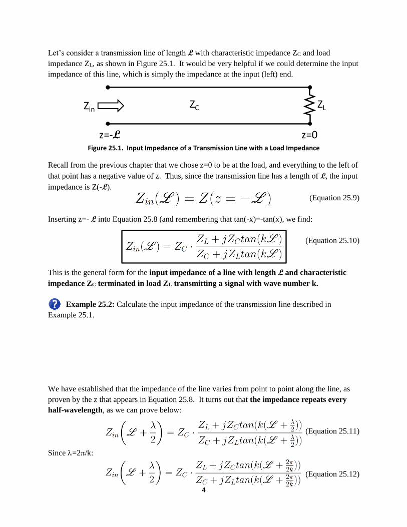
Let’s consider a transmission line of length L with characteristic impedance ZC and load

impedance ZL, as shown in Figure 25.1. It would be very helpful if we could determine the input

impedance of this line, which is simply the impedance at the input (left) end.

Figure 25.1. Input Impedance of a Transmission Line with a Load Impedance

Recall from the previous chapter that we chose z=0 to be at the load, and everything to the left of

that point has a negative value of z. Thus, since the transmission line has a length of L, the input

impedance is Z(-L).

(Equation 25.9)

Inserting z=- L into Equation 25.8 (and remembering that tan(-x)=-tan(x), we find:

(Equation 25.10)

This is the general form for the input impedance of a line with length L and characteristic

impedance ZC terminated in load ZL transmitting a signal with wave number k.

Example 25.2: Calculate the input impedance of the transmission line described in

Example 25.1.

We have established that the impedance of the line varies from point to point along the line, as

proven by the z that appears in Equation 25.8. It turns out that the impedance repeats every

half-wavelength, as we can prove below:

(Equation 25.11)

Since =2/k:

(Equation 25.12)

ZLZC

z=0z=-L

Zin

5

Simplifying gives:

(Equation 25.13)

Since tan(+)=tan(), we find:

(Equation 25.14)

Combined with Equation 25.10, this allows us to prove that:

(Equation 25.15)

It also turns out that the input impedance of a line that is one-quarter wavelength (/4) long has

a special value. Beginning with Equation 25.10, we find:

(Equation 25.16)

Substituting k=2/, we find:

(Equation 25.17)

Simplifying gives:

(Equation 25.18)

But we know that tan(/2)=∞, so we can write:

(Equation 25.19)

(Technically, we shouldn’t write ∞ in an equation like this. It’s actually a limit.) The infinite

terms in the numerator and denominator will overwhelm the non-infinite terms, giving:

(Equation 25.20)

Since both infinities represent the same function, they will cancel, leaving:

6

(Equation 25.21)

This is a very special result, which we will use in upcoming calculations several times.

Let’s also consider the input impedance of the three special cases of a transmission line

termination: impedance matched, short-circuited, and open-circuited.

If the transmission line is impedance matched (ZL=ZC), then Equation 25.10 becomes:

(Equation 25.22)

Since the numerator and denominator are identical, they cancel out, leaving:

(Equation 25.23)

Thus, for an impedance-matched transmission line, the input impedance is equal to the

characteristic impedance.

If the transmission line is short-circuited (ZL=0), Equation 25.10 becomes:

(Equation 25.24)

This reduces to:

(Equation 25.25)

This is the input impedance of a short-circuited transmission line.

Example 25.3: Calculate the input impedance of the transmission line described in

Example 25.1 if it is short-circuited rather than terminated with an impedance of 50.

7

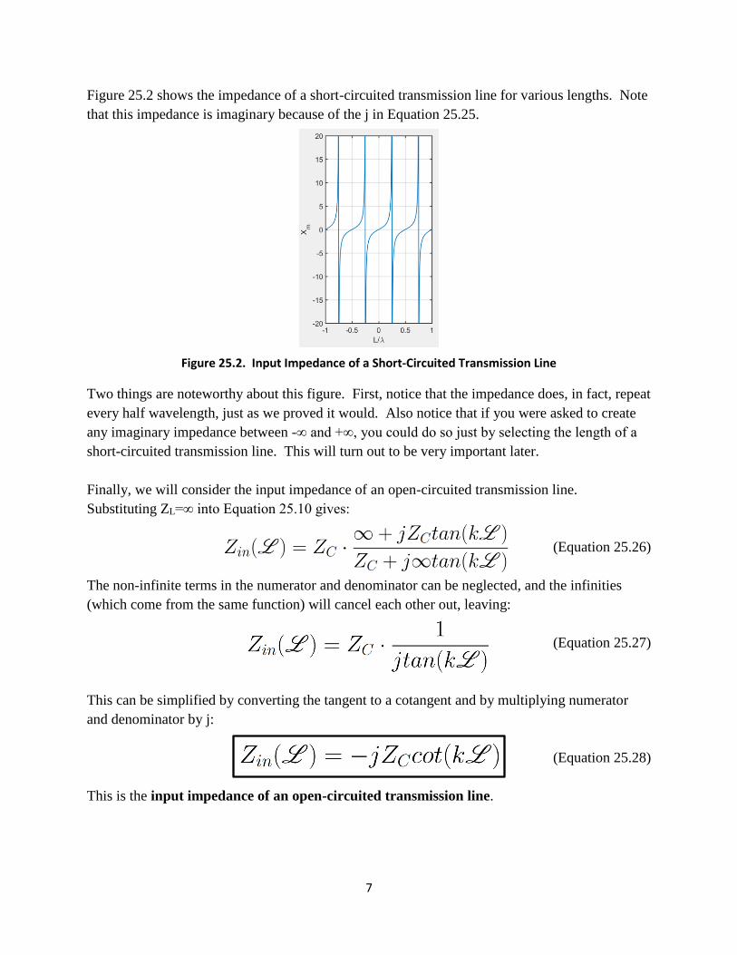
Figure 25.2 shows the impedance of a short-circuited transmission line for various lengths. Note

that this impedance is imaginary because of the j in Equation 25.25.

Figure 25.2. Input Impedance of a Short-Circuited Transmission Line

Two things are noteworthy about this figure. First, notice that the impedance does, in fact, repeat

every half wavelength, just as we proved it would. Also notice that if you were asked to create

any imaginary impedance between -∞ and +∞, you could do so just by selecting the length of a

short-circuited transmission line. This will turn out to be very important later.

Finally, we will consider the input impedance of an open-circuited transmission line.

Substituting ZL=∞ into Equation 25.10 gives:

(Equation 25.26)

The non-infinite terms in the numerator and denominator can be neglected, and the infinities

(which come from the same function) will cancel each other out, leaving:

(Equation 25.27)

This can be simplified by converting the tangent to a cotangent and by multiplying numerator

and denominator by j:

(Equation 25.28)

This is the input impedance of an open-circuited transmission line.

8

Example 25.4: Calculate the input impedance of the transmission line described in

Example 25.1 if it is open-circuited.

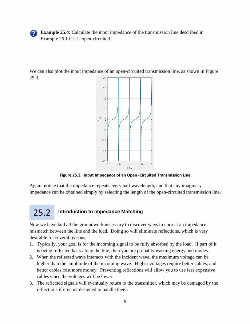
We can also plot the input impedance of an open-circuited transmission line, as shown in Figure

25.3.

Figure 25.3. Input Impedance of an Open -Circuited Transmission Line

Again, notice that the impedance repeats every half wavelength, and that any imaginary

impedance can be obtained simply by selecting the length of the open-circuited transmission line.

Introduction to Impedance Matching

Now we have laid all the groundwork necessary to discover ways to correct an impedance

mismatch between the line and the load. Doing so will eliminate reflections, which is very

desirable for several reasons:

1. Typically, your goal is for the incoming signal to be fully absorbed by the load. If part of it

is being reflected back along the line, then you are probably wasting energy and money.

2. When the reflected wave interacts with the incident wave, the maximum voltage can be

higher than the amplitude of the incoming wave. Higher voltages require better cables, and

better cables cost more money. Preventing reflections will allow you to use less expensive

cables since the voltages will be lower.

3. The reflected signals will eventually return to the transmitter, which may be damaged by the

reflections if it is not designed to handle them.

25.2

9

4. It is very likely that the reflected wave will also reflect off the left end of the wire, which will

create an echo of the original signal some time later. This can create interference with new

signals that are incoming at the same time.

For these three reasons, we really want to reduce or eliminate reflections, which means the load

impedance must match the characteristic impedance. But we don’t always control either of those

quantities. Maybe the transmission line is very hard to replace, or it is prohibitively expensive to

do so. Most of the time, the load impedance is set, and you can’t do anything to change it. So

what can we do?

There are three strategies we can apply. Each of them involves making a small change at or near

the load end of the wire to make it look like the load impedance matches the line impedance,

even when it doesn’t actually match. Each of these strategies has strengths and weaknesses,

although one of them does seem to be better than the other two. The strategies are:

1. Using a Quarter-Wave Transformer

2. Inserting a Parallel Load

3. Designing a Single-Stub Tuner

We will consider each of these solutions, along with their strengths and weaknesses, in the

following three sections.

Quarter-Wave Transformers

As you may recall from Equation 25.21, quarter-wave transmission lines exhibit a special input

impedance:

(Copy of Equation 25.21)

We can use this to our advantage by inserting a quarter-wavelength piece of transmission line

between the end of the transmission line and the load to change the apparent impedance of the

load. This is illustrated in Figure 25.4.

Figure 25.4. Impedance Matching with a Quarter-Wave Transformer

Notice that we already know every quantity in this figure except ZC(/4), which is the

characteristic impedance of the short piece of cable we will be adding.

25.3

ZL

ZCZC (/4)

Z2

10

If we “look into” the wire from the left of the quarter-wave transformer, we will see impedance

Z2, as shown in the Figure. We can calculate Z2 from Equation 25.21:

(Equation 25.29)

In order for the line to be impedance matched, we must ensure that Z2, the impedance seen as the

load to the main wire, is equal to ZC:

(Equation 25.30)

Solving this equation for ZC(/4) gives:

(Equation 25.31)

Example 25.5: Calculate the characteristic impedance and length of a quarter-wave

transformer for the situation in Example 25.1.

The quarter-wave transformer has one substantial shortcoming. It requires specifying a very

precise characteristic impedance for the transformer, and transmission lines are usually only

available in a few pre-determined impedances. This means that a 73.5W transmission line to

form a quarter-wave transformer would very likely have to be custom-made, which would be

very expensive.

Parallel Load Matching

A second solution is to add a second load in parallel with the original load, and selecting the

parallel load such that the combination of the original load and that of the parallel load combine

together to match the line impedance. This is shown in Figure 25.5.

25.4

11

Figure 25.5. Impedance Matching with a Parallel Load

Here, ZL is the original load, ZQ is the parallel load, and Z2 is the combined load, which must

equal the line impedance ZC. This requirement can be written in the following equation:

(Equation 25.32)

Solving this equation for the unknown quantity ZQ gives:

(Equation 25.33)

This is the amount of impedance that must be placed at the load in order to match it to a

smaller line impedance.

Example 25.6: Calculate the parallel load that would be needed to match a 100 load to a

75 line.

Since these impedances are being added in parallel, it might be easier to work with admittances

(the reciprocal of impedance, represented by Y). In that case, Equation 25.33 can be written as:

(Equation 25.34)

This strategy will only work if the load impedance is higher than the line impedance, since

adding another impedance in parallel can only decrease the load impedance, not increase it. If

the load impedance is too low, we will need to place the parallel load one quarter wavelength

away from the load, as shown in Figure 25.6.

ZLZC

z=0

ZQ

Z2

12

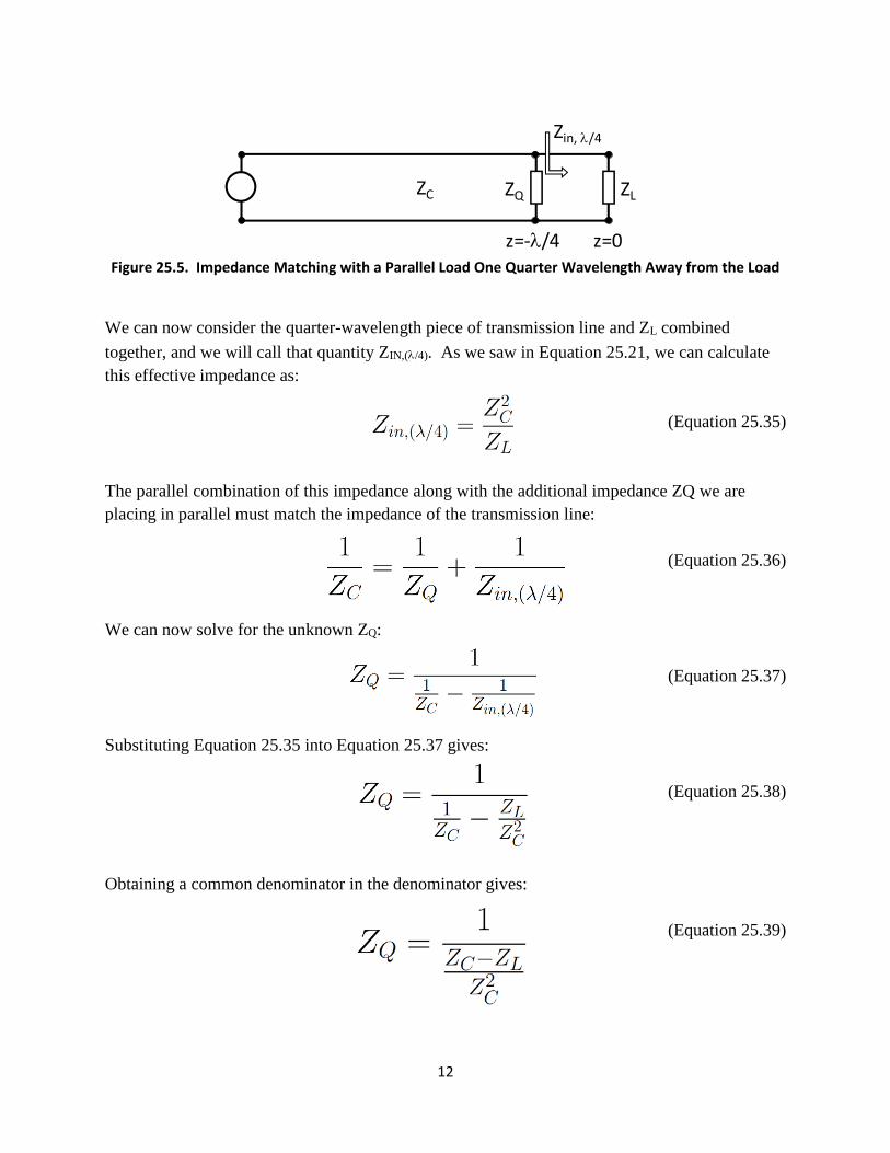
Figure 25.5. Impedance Matching with a Parallel Load One Quarter Wavelength Away from the Load

We can now consider the quarter-wavelength piece of transmission line and ZL combined

together, and we will call that quantity ZIN,(/4). As we saw in Equation 25.21, we can calculate

this effective impedance as:

(Equation 25.35)

The parallel combination of this impedance along with the additional impedance ZQ we are

placing in parallel must match the impedance of the transmission line:

(Equation 25.36)

We can now solve for the unknown ZQ:

(Equation 25.37)

Substituting Equation 25.35 into Equation 25.37 gives:

(Equation 25.38)

Obtaining a common denominator in the denominator gives:

(Equation 25.39)

ZLZC

z=0

ZQ

z=-/4

Zin, /4

13

Simplifying this expression gives:

(Equation 25.40)

This is the amount of impedance that must be placed one-quarter wavelength away from the

load in order to match the load impedance to a larger line impedance.

Alternatively, you could perform the calculation using admittances as in the previous section.

(Equation 25.41)

Example 25.7: What impedance would be needed, and where would it need to be placed,

in order to match the load and the line in Example 25.1?

Parallel load matching is typically a better option than quarter-wave transformers. The main

problem here is that the parallel load ZQ is necessarily going to absorb some of the power coming

from the source. There will be no reflections on the line, but less than 100% of the power will be

delivered to the load.

Single-Stub Tuner Matching

The third and final method for impedance matching is to insert a single-stub tuner. This tuner

will involve inserting a short piece of the very same transmission line we are working with at

precisely the correct location and with precisely the correct length. The stub can be either short-

circuited or open-circuited, but in practice it is short-circuited because an open-circuited stub

tends to radiate electromagnetic waves. In other words, an open-circuited stub acts like an

antenna, which can create all kinds of other problems. Short-circuited stubs don’t do this, which

is why we use them.

As you hopefully remember from Equation 25.25 and Figure 25.2, a short-circuited piece of

transmission line can be designed to act like any amount of imaginary impedance simply by

selecting the length correctly. In this way, a single-stub tuner is similar to a parallel load, except

25.5

14

the load being added in parallel is a short-circuited transmission line, and its imaginary

impedance will not absorb any of the power from the signal source.

Figure 25.6 illustrates a single-stub tuner.

Figure 25.6. Impedance Matching with a Single-Stub Tuner

Our job is to select d1 and d2 such that ZIN1 in parallel with ZIN2 is equal to ZC. Mathematically,

this will be easiest to do if we work with admittances rather than impedances:

(Equation 25.42)

We know from Equation 25.25 that the admittance of the short-circuited stub is:

(Equation 25.43)

Equation 25.10 can be used to determine the admittance of the line to the right of the stub, along

with the load impedance:

(Equation 25.44)

Substituting Equations 25.43 and 25.44 into Equation 25.42 gives:

(Equation 25.45)

Multiplying both sides by ZC gives:

(Equation 25.46)

Zin2

d1

d2

ZLZC

Zin1

15

Multiplying each side by the product of the denominators on the left side gives an equation with

no fractions:

(Equation 25.47)

Multiplying out both sides of this equations gives:

(Equation 25.48)

This complex equation can only be true if the real parts on both side are equal to each other and

the imaginary parts on both sides are equal to each other. We will consider the imaginary parts

first:

(Equation 25.49)

Dividing by j and grouping the d2 terms on the same side gives:

(Equation 25.50)

Dividing by ZC isolates the tan(kd1) term:

(Equation 25.51)

This equation gives one relationship between d1 and d2 in terms of k, ZL, and ZC. We have two

unknowns, so we need two equations. We will get the second equation by setting the real parts

of Equation 25.48 equal to each other:

(Equation 25.52)

Rearranging gives:

(Equation 25.53)

Substituting Equation 25.51 into Equation 25.53 gives:

(Equation 25.54)

Simplifying:

(Equation 25.55)

16

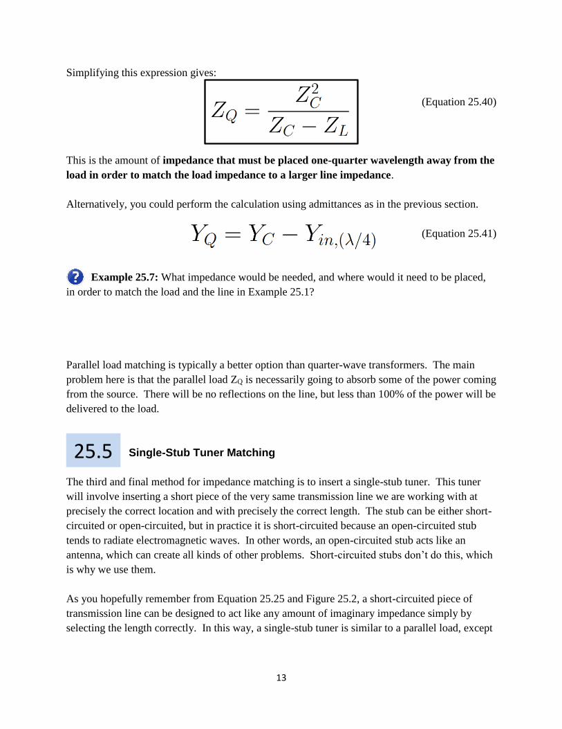
Solving for d2 gives:

(Equation 25.56)

We can then solve Equation 25.51 for d1 in terms of k, ZL, ZC, and d2:

(Equation 25.57)

Note that you must solve for d2 first, since it is required in the equation for d1. Also, be aware

that the most common error when solving a problem like this one is to The quantity d1 is the

distance from the load where the stub must be placed, and d2 is the required length of the

stub.

Example 25.8: Design a single-stub tuner to minimize reflections in a 75 coaxial cable

with a relative dielectric constant of 4 that is terminated with a load impedance of 100. It is

driven by a function generator operating at 125MHz. Assume the stub is short-circuited and is

made of the same material as the line itself.

17

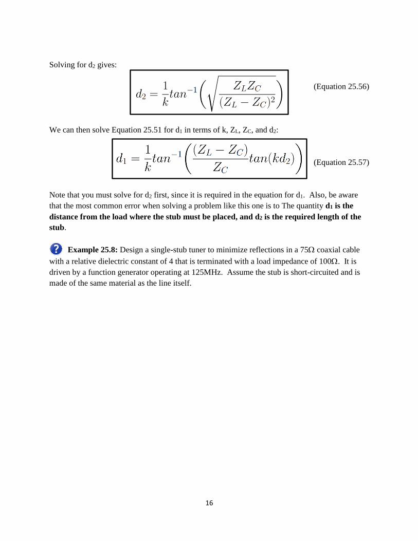
Summary

The impedance (the ratio of the total voltage to the total current) varies from point to point

along a line. The following equation can be used to calculate the impedance at any point:

The input impedance of a line with length L and characteristic impedance ZC terminated in

load ZL transmitting a signal with wave number k is:

The impedance repeats every half-wavelength:

If the line is a quarter-wavelength long, then there is a special expression for the input

impedance:

The input impedance of a short-circuited transmission line is:

The input impedance of an open-circuited transmission line is:

A quarter-wave transformer can match the load to the line if it is exactly a quarter-

wavelength long and has a characteristic impedance determined by:

If the load impedance is greater than the line impedance, a parallel load can be placed right at

the original load with a value of:

25.6

18

If the load impedance is less than the line impedance, the parallel load must be placed a

quarter-wavelength back from the load, and it must have an impedance of:

A single stub tuner made of the same material as the original line must be placed a

distance d1 away from the load and must have a length of d2: