420 Part VI Learning About the World Chapter 25 – Paired Samples and Blocks 1. More eggs? a) Randomly assign 50 hens to each of the two kinds of feed. Compare the mean egg production of the two groups at the end of one month. b) Randomly divide the 100 hens into two groups of 50 hens each. Feed the hens in the first group the regular feed for two weeks, then switch to the additive for 2 weeks. Feed the hens in the second group the additive for two weeks, and then switch to the regular feed for two weeks. Subtract each hen’s “regular” egg production from her “additive” egg production, and analyze the mean difference in egg production. c) The matched pairs design in part b is the stronger design. Hens vary in their egg production regardless of feed. This design controls for that variability by matching the hens with themselves. 2. MTV. a) Randomly assign half of the volunteers to do the puzzles in a quiet room, and assign the other half to do the puzzles with MTV on. Compare the mean time of the group in the quiet room to the mean time of the group watching MTV. b) Randomly assign half of the volunteers to do a puzzle in a quiet room, and assign the other half to do the puzzles with MTV on. Then have each do a puzzle under the other condition. Subtract each volunteer’s “quiet” time from his or her “MTV” time, and analyze the mean difference in times. Copyright 2010 Pearson Education, Inc.
Transcript
420 Part VI Learning About the World
Chapter 25 – Paired Samples and Blocks
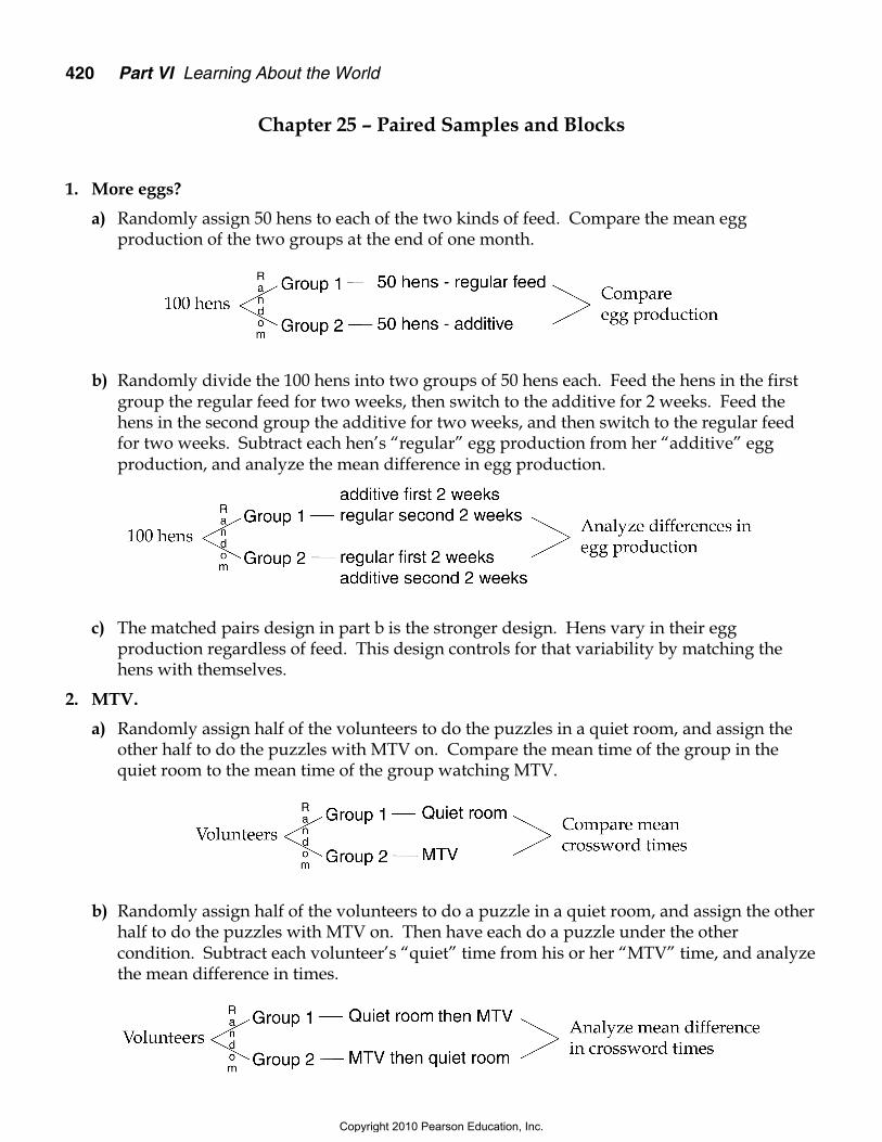
1. More eggs?
a) Randomly assign 50 hens to each of the two kinds of feed. Compare the mean eggproduction of the two groups at the end of one month.
b) Randomly divide the 100 hens into two groups of 50 hens each. Feed the hens in the firstgroup the regular feed for two weeks, then switch to the additive for 2 weeks. Feed thehens in the second group the additive for two weeks, and then switch to the regular feedfor two weeks. Subtract each hen’s “regular” egg production from her “additive” eggproduction, and analyze the mean difference in egg production.
c) The matched pairs design in part b is the stronger design. Hens vary in their eggproduction regardless of feed. This design controls for that variability by matching thehens with themselves.
2. MTV.
a) Randomly assign half of the volunteers to do the puzzles in a quiet room, and assign theother half to do the puzzles with MTV on. Compare the mean time of the group in thequiet room to the mean time of the group watching MTV.
b) Randomly assign half of the volunteers to do a puzzle in a quiet room, and assign the otherhalf to do the puzzles with MTV on. Then have each do a puzzle under the othercondition. Subtract each volunteer’s “quiet” time from his or her “MTV” time, and analyzethe mean difference in times.
Copyright 2010 Pearson Education, Inc.
Chapter 25 Paired Samples and Blocks 421
c) The matched pairs design in part b is the stronger design. People vary in their ability to docrossword puzzles. This design controls for that variability by matching the volunteerswith themselves.
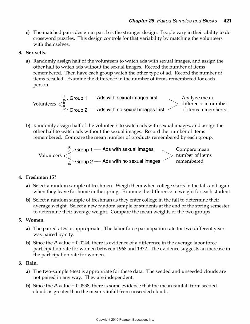
3. Sex sells.
a) Randomly assign half of the volunteers to watch ads with sexual images, and assign theother half to watch ads without the sexual images. Record the number of itemsremembered. Then have each group watch the other type of ad. Record the number ofitems recalled. Examine the difference in the number of items remembered for eachperson.
b) Randomly assign half of the volunteers to watch ads with sexual images, and assign theother half to watch ads without the sexual images. Record the number of itemsremembered. Compare the mean number of products remembered by each group.
4. Freshman 15?
a) Select a random sample of freshmen. Weigh them when college starts in the fall, and againwhen they leave for home in the spring. Examine the difference in weight for each student.
b) Select a random sample of freshman as they enter college in the fall to determine theiraverage weight. Select a new random sample of students at the end of the spring semesterto determine their average weight. Compare the mean weights of the two groups.
5. Women.
a) The paired t-test is appropriate. The labor force participation rate for two different yearswas paired by city.
b) Since the P-value = 0.0244, there is evidence of a difference in the average labor forceparticipation rate for women between 1968 and 1972. The evidence suggests an increase inthe participation rate for women.
6. Rain.
a) The two-sample t-test is appropriate for these data. The seeded and unseeded clouds arenot paired in any way. They are independent.
b) Since the P-value = 0.0538, there is some evidence that the mean rainfall from seededclouds is greater than the mean rainfall from unseeded clouds.
Copyright 2010 Pearson Education, Inc.
422 Part VI Learning About the World
7. Friday the 13th Part I:
a) The paired t-test is appropriate, since we have pairs of Fridays in 5 different months. Datafrom adjacent Fridays within a month may be more similar than randomly chosen Fridays.
b) Since the P-value = 0.0212, there is evidence that the mean number of cars on the M25motorway on Friday the 13th is less than the mean number of cars on the previous Friday.
c) We don’t know if these Friday pairs were selected at random. Obviously, if these are theFridays with the largest differences, this will affect our conclusion. The Nearly Normalcondition appears to be met by the differences, but the sample size of five pairs is small.
8. Friday the 13th, Part II:
a) The paired t-test is appropriate, since we have pairs of Fridays in 6 different months. Datafrom adjacent Fridays within a month may be more similar than randomly chosen Fridays.
b) Since the P-value = 0.0211, there is evidence that the mean number of admissions tohospitals found on Friday the 13th is more than on the previous Friday.
c) We don’t know if these Friday pairs were selected at random. Obviously, if these are theFridays with the largest differences, this will affect our conclusion. The Nearly Normalcondition appears to be met by the differences, but the sample size of six pairs is small.
9. Online insurance I.
Adding variances requires that the variables be independent. These price quotes are forthe same cars, so they are paired. Drivers quoted high insurance premiums by the localcompany will be likely to get a high rate from the online company, too.
10. Windy, part I.
Adding variances requires that the variables be independent. The wind speeds wererecorded at nearby sites, to they are likely to be both high or both low at the same time.
11. Online insurance II.
a) The histogram would help you decide whether the online company offers cheaperinsurance. We are concerned with the difference in price, not the distribution of each set ofprices.
b) Insurance cost is based on risk, so drivers are likely to see similar quotes from eachcompany, making the differences relatively smaller.
c) The price quotes are paired. They were for a random sample of fewer than 10% of theagent’s customers and the histogram of differences looks approximately Normal.
12. Windy, part II.
a) The outliers are particularly windy days, but they were windy at both sites, making thedifference in wind speeds less unusual.
b) The histogram and summaries of the differences are more appropriate because they arepaired observations and all we care about is which site is windier.
Copyright 2010 Pearson Education, Inc.
Chapter 25 Paired Samples and Blocks 423
c) The wind measurements at the same times at tow nearby sites are paired. We should beconcerned that there might be a lack of independence from one time to the next, but thetimes were 6 hours apart and the differences in speeds are likely to be independent.Although not random, we can regard a sample this large as generally representative ofwind speed s at these sites. The histograms of differences is unimodal, symmetric and bell-shaped.
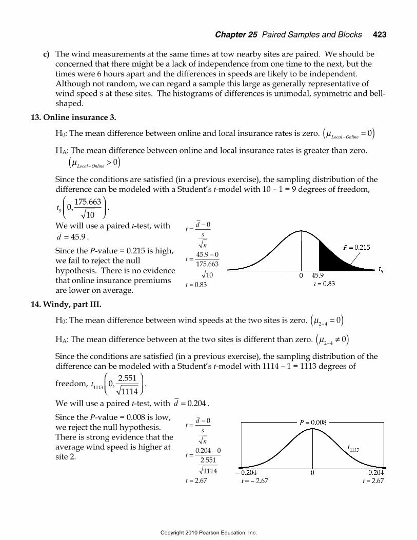
13. Online insurance 3.
H0: The mean difference between online and local insurance rates is zero. µLocal Online− =( )0
HA: The mean difference between online and local insurance rates is greater than zero.µ
Local Online− >( )0
Since the conditions are satisfied (in a previous exercise), the sampling distribution of thedifference can be modeled with a Student’s t-model with 10 – 1 = 9 degrees of freedom,
t9 0175 663
10,
.
.
We will use a paired t-test, withd = 45 9. .
Since the P-value = 0.215 is high,we fail to reject the nullhypothesis. There is no evidencethat online insurance premiumsare lower on average.
14. Windy, part III.
H0: The mean difference between wind speeds at the two sites is zero. µ2 4 0− =( )HA: The mean difference between at the two sites is different than zero. µ2 4 0− ≠( )Since the conditions are satisfied (in a previous exercise), the sampling distribution of thedifference can be modeled with a Student’s t-model with 1114 – 1 = 1113 degrees of
freedom, t1113 02 551
1114,
.
.
We will use a paired t-test, with d = 0 204. .
Since the P-value = 0.008 is low,we reject the null hypothesis.There is strong evidence that theaverage wind speed is higher atsite 2.
td
s
n
t
t
= −
= −
≈
0
45 9 0175 663
100 83
..
.
td
s
n
t
t
= −
= −
≈
0
0 204 02 551
11142 67
..
.
Copyright 2010 Pearson Education, Inc.
424 Part VI Learning About the World
15. Temperatures.
Paired data assumption: The data are paired by city.Randomization condition: These cities might not be representativeof all European cities, so be cautious in generalizing the results.10% condition: 12 cities are less than 10% of all European cities.Normal population assumption: The histogram of differencesbetween January and July mean temperature is roughly unimodaland symmetric.
Since the conditions are satisfied, the sampling distribution of thedifference can be modeled with a Student’s t-model with 12 – 1 = 11degrees of freedom. We will find a paired t-interval, with 90% confidence.
d ts
ntn
d±
= ±
≈−
∗ ∗1 1136 8333
8 6637512
32 3 41 3..
( . , . )
We are 90% confident that the average high temperature in European cities in July is anaverage of between 32.3° to 41.4° higher than in January.
16. Marathons 2006.
Paired data assumption: The data are paired by year.Randomization condition: Assume these years, at this marathon, arerepresentative of all differences.10% condition: 29 years is less than 10% of years for all marathons.Normal population assumption: The histogram of differencesbetween women’s and men’s times is roughly unimodal andsymmetric.
Since the conditions are satisfied, the sampling distribution of thedifference can be modeled with a Student’s t-model with 29 – 1 = 28 degrees of freedom.We will find a paired t-interval, with 90% confidence.
d ts
nt
nd±
= ±
−
∗ ∗1 2816 8517
1 89805
29.
. ≈ ( . , . )16 25 17 45
We are 90% confident women’s winning marathon times are an average of between 16.25and 17.45 minutes higher than men’s winning times.
17. Push-ups.
Independent groups assumption: The group ofboys is independent of the group of girls.Randomization condition: Assume that studentsare assigned to gym classes at random.10% condition: 12 boys and 12 girls are less than10% of all kids.Nearly Normal condition: The histograms of thenumber of push-ups from each group are roughlyunimodal and symmetric.
20 40 60
1
2
3
4
5
July-Jan
0 20 40
1
2
3
4
5
Girls
7 23 39
1
2
3
4
5
Boys
11.25 16.25 21.25
2
4
6
8
Women-Men
Copyright 2010 Pearson Education, Inc.
Chapter 25 Paired Samples and Blocks 425
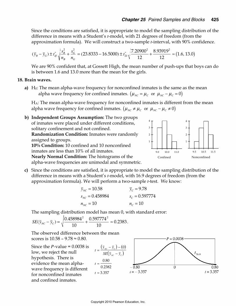
Since the conditions are satisfied, it is appropriate to model the sampling distribution of thedifference in means with a Student’s t-model, with 21 degrees of freedom (from theapproximation formula). We will construct a two-sample t-interval, with 90% confidence.
( ) ( . . ). .
. , .y y ts
n
s
ntB G df
B
B
G
G
− ± + = − ± + ≈ ( )∗ ∗2 2
21
2 2
23 8333 16 50007 20900
128 93919
121 6 13 0
We are 90% confident that, at Gossett High, the mean number of push-ups that boys can dois between 1.6 and 13.0 more than the mean for the girls.
18. Brain waves.
a) H0: The mean alpha-wave frequency for nonconfined inmates is the same as the meanalpha wave frequency for confined inmates. µ µ µ µNC C NC C= − =( ) or 0
HA: The mean alpha-wave frequency for nonconfined inmates is different from the meanalpha wave frequency for confined inmates. µ µ µ µNC C NC C≠ − ≠( ) or 0
b) Independent Groups Assumption: The two groupsof inmates were placed under different conditions,solitary confinement and not confined.Randomization Condition: Inmates were randomlyassigned to groups.10% Condition: 10 confined and 10 nonconfinedinmates are less than 10% of all inmates.Nearly Normal Condition: The histograms of thealpha-wave frequencies are unimodal and symmetric.
c) Since the conditions are satisfied, it is appropriate to model the sampling distribution of thedifference in means with a Student’s t-model, with 16.9 degrees of freedom (from theapproximation formula). We will perform a two-sample t-test. We know:
y
s
n
NC
NC
NC
===
10 58
0 458984
10
.
.
y
s
n
C
C
C
===
9 78
0 597774
10
.
.
The sampling distribution model has mean 0, with standard error:
SE y yNC C( ). .
.− = + ≈0 45898410
0 59777410
0 23832 2
.
The observed difference between the meanscores is 10.58 – 9.78 ≈ 0.80.
Since the P-value = 0.0038 islow, we reject the nullhypothesis. There isevidence the mean alpha-wave frequency is differentfor nonconfined inmatesand confined inmates.
9.5 10.5 11.5
1
2
3
4
Nonconfined
9.0 10.0 11.0
1
2
3
4
Confined
ty y
SE y y
t
t
NC C
NC C
=− −
−
≈
≈
( ) ( )( )
0
0 80
0 23823 357
.
.
.
Copyright 2010 Pearson Education, Inc.
426 Part VI Learning About the World
d) The evidence suggests that the mean alpha-wave frequency for inmates subjected toconfinement is diffrent than the mean alpha-wave frequency for inmates that are notconfined. This experiment suggests that mean alpha-wave frequency is lower for confinedinmates.
19. Job satisfaction.
a) Use a paired t-test.
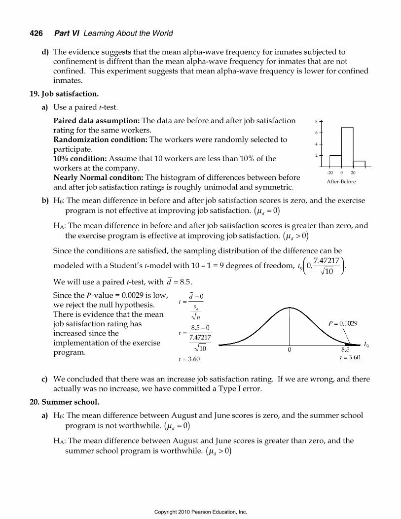
Paired data assumption: The data are before and after job satisfactionrating for the same workers.Randomization condition: The workers were randomly selected toparticipate.10% condition: Assume that 10 workers are less than 10% of theworkers at the company.Nearly Normal conditon: The histogram of differences between beforeand after job satisfaction ratings is roughly unimodal and symmetric.
b) H0: The mean difference in before and after job satisfaction scores is zero, and the exerciseprogram is not effective at improving job satisfaction. µd =( )0
HA: The mean difference in before and after job satisfaction scores is greater than zero, andthe exercise program is effective at improving job satisfaction. µd >( )0
Since the conditions are satisfied, the sampling distribution of the difference can be
modeled with a Student’s t-model with 10 – 1 = 9 degrees of freedom, t9 07 47217
10,
.
.
We will use a paired t-test, with d = 8 5. .
Since the P-value = 0.0029 is low,we reject the null hypothesis.There is evidence that the meanjob satisfaction rating hasincreased since theimplementation of the exerciseprogram.
c) We concluded that there was an increase job satisfaction rating. If we are wrong, and thereactually was no increase, we have committed a Type I error.
20. Summer school.
a) H0: The mean difference between August and June scores is zero, and the summer schoolprogram is not worthwhile. µd =( )0
HA: The mean difference between August and June scores is greater than zero, and thesummer school program is worthwhile. µd >( )0
-20 0 20
2
4
6
8
After-Before
td
s
n
t
t
d
=−
=−
≈
0
8 5 07 47217
10
3 60
.
.
.
Copyright 2010 Pearson Education, Inc.
Chapter 25 Paired Samples and Blocks 427
Paired data assumption: The scores are paired by student.Randomization condition: Assume that these students arerepresentative of students who attend this school in other years.10% condition: 6 students are less than 10% of all students.Normal population assumption: The histogram of differencesbetween August and June scores shows a distribution that couldhave come from a Normal population.
Since the conditions are satisfied, the sampling distribution of thedifference can be modeled with a Student’s t-model with 6 – 1 = 5 degrees of freedom,
t5 07 44759
6,
.
.
We will use a paired t-test, withd = 5 3. .
Since the P-value = 0.0699 isfairly high, we fail to reject thenull hypothesis. There is notstrong evidence that scoresincreased on average. The summer school program does not appear worthwhile, but theP-value is low enough that we should look at a larger sample to be more confident in ourconclusion.
b) We concluded that there was no evidence of an increase. If there actually was an increase,we have committed a Type II error.
21. Yogurt.
H0: The mean difference in calories between servings of strawberry and vanilla yogurt iszero. µd =( )0
HA: The mean difference in calories between servings of strawberry and vanilla yogurt isdifferent from zero. µd ≠( )0
Paired data assumption: The yogurt is paired bybrand.Randomization condition: Assume that these brandsare representative of all brands.10% condition: 12 brands of yogurt might not be lessthan 10% of all brands of yogurt. Proceed cautiously.Normal population assumption: The histogram ofdifferences in calorie content between strawberry andvanilla shows an outlier, Great Value. When theoutlier is eliminated, the histogram of differences isroughly unimodal and symmetric.
-5 0 5 10 15 20
1
2
Aug-Jun
td
s
n
t
t
d
=−
=−
≈
0
5 3 07 44759
6
1 75
.
.
.
-25 -5 15 35
1
2
3
4
5
S-V
-25 5 35 65 95
1
2
3
4
5
S-V
With outlier Without outlier
Copyright 2010 Pearson Education, Inc.
428 Part VI Learning About the World
When Great Value yogurt is removed, the conditions are satisfied. The samplingdistribution of the difference can be modeled with a Student’s t-model with
11 – 1 = 10 degrees of freedom, t10 018 0907
11,
.
.
We will use a paired t-test, with d ≈ 4 54545. .
Since the P-value = 0.4241 ishigh, we fail to reject the nullhypothesis. There is noevidence of a mean differencein calorie content betweenstrawberry yogurt and vanillayogurt.
22. Gasoline.
a) H0: The mean difference in mileage between premium and regular is zero. µd =( )0
HA: The mean difference in mileage between premium and regular is greater than zero.µd >( )0
Paired data assumption: The mileage is paired by car.Randomization condition: We randomized the order in which thedifferent types of gasoline were used in each car.10% condition: We are testing the mileage, not the car, so we don’tneed to check this condition.Normal population assumption: The histogram of differencesbetween premium and regular is roughly unimodal and symmetric.
Since the conditions are satisfied, the sampling distribution of the difference can be
modeled with a Student’s t-model with 10 – 1 = 9 degrees of freedom, t9 01 41421
10,
.
.
We will use a paired t-test, with d = 2.
Since the P-value = 0.0008 isvery low, we reject the nullhypothesis. There is strongevidence of a mean increase ingas mileage between regularand premium.
-2.5 0.0 2.5 5.0
1
2
3
4
5
Prem.- Reg.
td
s
n
t
t
d
=−
=−
≈
0
2 01 41421
10
4 47
.
.
td
s
n
t
t
d
=−
=−
≈
0
4 54545 018 0907
11
0 833
.
.
.
Copyright 2010 Pearson Education, Inc.
Chapter 25 Paired Samples and Blocks 429
b) d ts
ntn
d±
= ±
≈−
∗ ∗1 92
1 4142110
1 18 2 82.
( . , . )
We are 90% confident that the mean increase in gas mileage when using premium ratherthan regular gasoline is between 1.18 and 2.82 miles per gallon.
c) Premium costs more than regular. This difference might outweigh the increase in mileage.
d) With t = 1.25 and a P-value = 0.1144, we would have failed to reject the null hypothesis,and conclude that there was no evidence of a mean difference in mileage. The variation inperformance of individual cars is greater than the variation related to the type of gasoline.This masked the true difference in mileage due to the gasoline. (Not to mention the factthat the two-sample test is not appropriate because we don’t have independent samples!)
23. Braking.
a) Randomization Condition: These cars are not a random sample, but are probablyrepresentative of all cars in terms of stopping distance.10% Condition: These 10 cars are less than 10% of all cars.Nearly Normal Condition: A histogram of the stopping distances is skewed to the right,but this may just be sampling variation from a Normal population. The “skew” is only acouple of stopping distances. We will proceed cautiously.
The cars in the sample had a mean stopping distance of 138.7 feet and a standard deviationof 9.66149 feet. Since the conditions have been satisfied, construct a one-sample t-interval,with 10 – 1 = 9 degrees of freedom, at 95% confidence.
y ts
ntn±
= ±
≈−
∗ ∗1 9138 7
9 6614910
131 8 145 6..
( . , . )
We are 95% confident that the mean dry pavement stopping distance for cars with this typeof tires is between 131.8 and 145.6 feet. This estimate is based on an assumption that thesecars are representative of all cars and that the population of stopping distances is Normal.
b) Paired data assumption: The data are paired by car.Randomization condition: Assume that the cars are representative ofall cars.10% condition: The 10 cars tested are less than 10% of all cars.Normal population assumption: The difference in stopping distancefor car #4 is an outlier, at only 12 feet. After excluding this difference,the histogram of differences is unimodal and symmetric.
Since the conditions are satisfied, the sampling distribution of thedifference can be modeled with a Student’s t-model with 9 – 1 = 8 degrees of freedom. Wewill find a paired t-interval, with 95% confidence.
d ts
ntn
d±
= ±
≈−
∗ ∗1 855
10 21039
47 2 62 8.
( . , . )
With car #4 removed, we are 95% confident that the mean increase in stopping distance onwet pavement is between 47.2 and 62.8 feet. (If you leave the outlier in, the interval is 38.8to 62.6 feet, but you should remove it! This procedure is sensitive outliers!)
20 40 60
2
4
6
Wet-Dry
Copyright 2010 Pearson Education, Inc.
430 Part VI Learning About the World
24. Braking, test 2.
a) Randomization Condition: These stops are probably representative ofall such stops for this type of car, but not for all cars.10% Condition: 10 stops are less than 10% of all possible stops.Nearly Normal Condition: A histogram of the stopping distances isroughly unimodal and symmetric.
The stops in the sample had a mean stopping distance of 139.4 feet,and a standard deviation of 8.09938 feet. Since the conditions havebeen satisfied, construct a one-sample t-interval, with 10 – 1 = 9degrees of freedom, at 95% confidence.
y ts
ntn±
= ±
≈−
∗ ∗1 9139 4
8 0993810
133 6 145 2..
( . , . )
We are 95% confident that the mean dry pavement stopping distance for this type of car isbetween 133.6 and 145.2 feet.
b) Independent Groups Assumption: The wet pavement stops and dry pavement stops weremade under different conditions and not paired in any way.Randomization Condition: These stops are probably representative of all such stops forthis type of car, but not for all cars.10% Condition: 10 stops are less than 10% of allpossible stops.Nearly Normal Condition: The histogram of drypavement stopping distances is roughly unimodaland symmetric (from part a), but the histogram ofwet pavement stopping distances is a bit skewed.Since the Normal probability plot looks fairlystraight, we will proceed.
Since the conditions are satisfied, it is appropriate to model the sampling distribution of thedifference in means with a Student’s t-model, with 13.8 degrees of freedom (from theapproximation formula). We will construct a two-sample t-interval, with 95% confidence.
( ) ( . . ). .
. , ..y y ts
n
s
ntW D df
W
W
D
D
− ± + = − ± + ≈ ( )∗ ∗2 2
13 8
2 2
202 4 139 415 07168
108 09938
1051 4 74 6
We are 95% confident that the mean stopping distance on wet pavement is between 51.4and 74.6 feet longer than the mean stopping distance on dry pavement.
125 135 145 155
1
2
3
4
Dry
175 195 215
1
2
3
4
Wet
187.5
200.0
212.5
-1 0 1
nscores
Wet
Copyright 2010 Pearson Education, Inc.
Chapter 25 Paired Samples and Blocks 431
25. Tuition 2006.
a) Paired data assumption: The data are paired by college.Randomization condition: The colleges were selected randomly.Normal population assumption: The tuition difference for UCIrvine, at $9300, is an outlier. Once it has been set aside, thehistogram of the differences is roughly unimodal and symmetric.
Since the conditions are satisfied, the sampling distribution of thedifference can be modeled with a Student’s t-model with 18 – 1 = 17degrees of freedom. We will find a paired t-interval, with 90% confidence.
d ts
nt
nd±
= ±
−
∗ ∗1 173266 67
1588 56
18.
. ≈ ( . , . )2615 31 3918 02
b) With UC Irvine removed, we are 90% confident that the mean increase in tuition fornonresidents versus residents is between about $2615 and $3918. (If you left UC Irvine inyour data, the interval is about $2759 to $4409, but you should set it aside! This procedureis sensitive to the presence of outliers!)
c) There is no evidence to suggest that the magazine made a false claim. An increase of $3500for nonresidents is contained within our 90% confidence interval.
26. Sex sells, part II.
H0: The mean difference in number of items remembered for ads with sexual images andads without sexual images is zero. µd =( )0
HA: The mean difference in number of items remembered for ads with sexual images andads without sexual images is not zero. µd ≠( )0
Paired data assumption: The data are paired by subject.Randomization condition: The ads were in random order.Normal population assumption: The histogram of differences isroughly unimodal and symmetric.
Since the conditions are satisfied, the sampling distribution of thedifference can be modeled with a Student’s t-model with 39 – 1 = 38 degrees of freedom,
t38 01 677
39,
.
. We will use a paired t-test, with d = 0 231. .
Since the P-value = 0.3956 ishigh, we fail to reject the nullhypothesis. There is noevidence of a mean differencein the number of objectsremembered with ads withsexual images and without.
- 4 0 4
2
4
6
8
1 0
SI-Ns
td
s
n
t
t
d
=−
=−
≈
0
0 231 01 67747
39
0 86
.
.
.
0 4000
2
4
6
8
10
NRt-Rst
Copyright 2010 Pearson Education, Inc.
432 Part VI Learning About the World
27. Strikes.
a) Since 60% of 50 pitches is 30 pitches, the Little Leaguers would have to throw an average ofmore than 30 strikes in order to give support to the claim made by the advertisements.
H0: The mean number of strikes thrown by Little Leaguers who have completed thetraining is 30. µA =( )30
HA: The mean number of strikes thrown by Little Leaguers who have completed thetraining is greater than 30. µA >( )30
Randomization Condition: Assume that these players arerepresentative of all Little League pitchers.10% Condition: 20 pitchers are less than 10% of all Little Leaguepitchers.Nearly Normal Condition: The histogram of the number of strikesthrown after the training is roughly unimodal and symmetric.
The pitchers in the sample threw a mean of 33.15 strikes, with astandard deviation of 2.32322 strikes. Since the conditions for inferenceare satisfied, we can model the sampling distribution of the mean number of strikes
thrown with a Student’s t model, with 20 – 1 = 19 degrees of freedom, t19 302 32322
20,
.
.
We will perform a one-sample t-test.
Since the P-value = 3 92 10 6. × − is very low, we reject the null hypothesis.There is strong evidence that the mean number of strikes that LittleLeaguers can throw after the training is more than 30. (This test saysnothing about the effectiveness of the training; just that Little Leaguerscan throw more than 60% strikes on average after completing thetraining. This might not be an improvement.)
b) H0: The mean difference in number of strikes thrown before and after the training is zero.µd =( )0
HA: The mean difference in number of strikes thrown before and after the training isgreater than zero. µd >( )0
Paired data assumption: The data are paired by pitcher.Randomization condition: Assume that these players arerepresentative of all Little League pitchers.10% condition: 20 players are less than 10% of all players.Normal population assumption: The histogram of differences isroughly unimodal and symmetric.
28 32 36
2
4
6
8
After
ty
s
n
t
t
A
A
A
=−
=−
=
µ0
33 15 302 32322
20
6 06
.
.
.
-5.0 0.0 5.0
2
4
6
After-Before
Copyright 2010 Pearson Education, Inc.
Chapter 25 Paired Samples and Blocks 433
Since the conditions are satisfied, the sampling distribution of the difference can be
modeled with a Student’s t-model with 20 – 1 = 19 degrees of freedom, t19 03 32297
19,
.
.
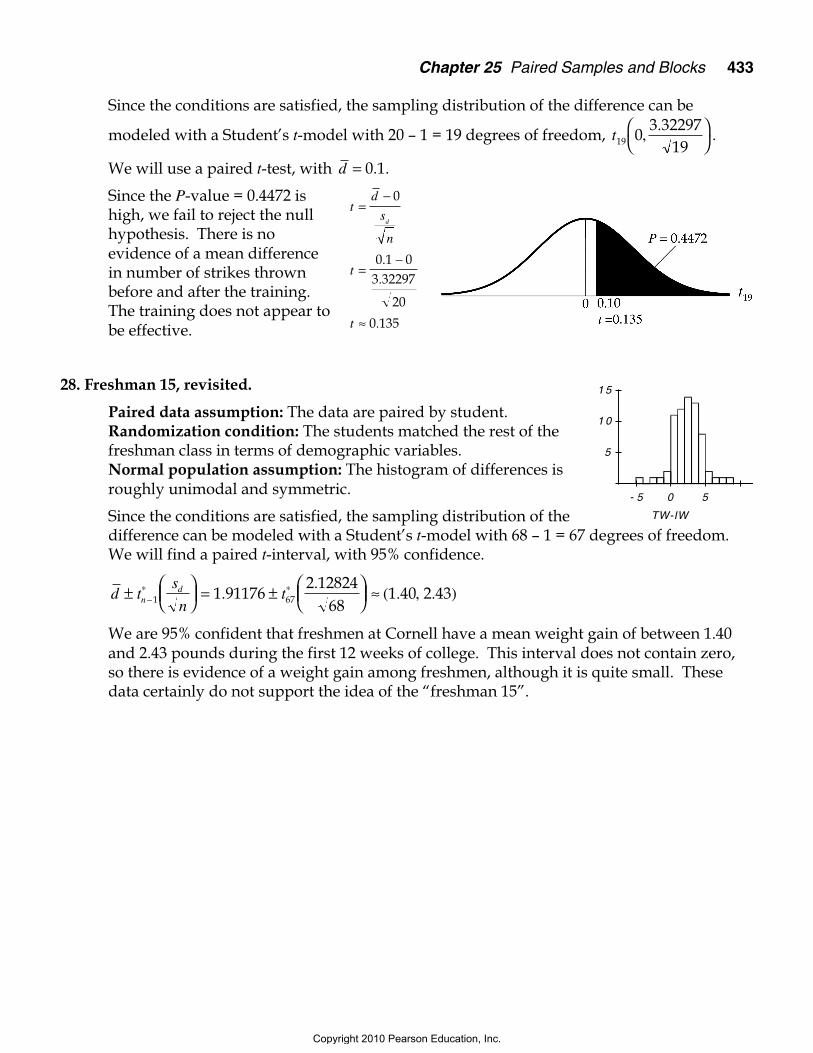
We will use a paired t-test, with d = 0 1. .
Since the P-value = 0.4472 ishigh, we fail to reject the nullhypothesis. There is noevidence of a mean differencein number of strikes thrownbefore and after the training.The training does not appear tobe effective.
28. Freshman 15, revisited.
Paired data assumption: The data are paired by student.Randomization condition: The students matched the rest of thefreshman class in terms of demographic variables.Normal population assumption: The histogram of differences isroughly unimodal and symmetric.
Since the conditions are satisfied, the sampling distribution of thedifference can be modeled with a Student’s t-model with 68 – 1 = 67 degrees of freedom.We will find a paired t-interval, with 95% confidence.
d ts
ntn
d±
= ±
≈−
∗ ∗1 671 91176
2 1282468
1 40 2 43..
( . , . )
We are 95% confident that freshmen at Cornell have a mean weight gain of between 1.40and 2.43 pounds during the first 12 weeks of college. This interval does not contain zero,so there is evidence of a weight gain among freshmen, although it is quite small. Thesedata certainly do not support the idea of the “freshman 15”.