chapter 2D rotation - avcr.czzoi.utia.cas.cz/files/chapter_2D_rotation.pdf · Chapter 3 2D Moment...

Chapter 3

2D Moment Invariants to

Translation, Rotation, and

Scaling

3.1 Introduction

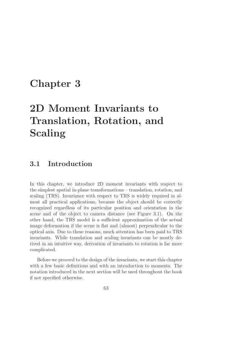
In this chapter, we introduce 2D moment invariants with respect tothe simplest spatial in-plane transformations – translation, rotation, andscaling (TRS). Invariance with respect to TRS is widely required in al-most all practical applications, because the object should be correctlyrecognized regardless of its particular position and orientation in thescene and of the object to camera distance (see Figure 3.1). On theother hand, the TRS model is a sufficient approximation of the actualimage deformation if the scene is flat and (almost) perpendicular to theoptical axis. Due to these reasons, much attention has been paid to TRSinvariants. While translation and scaling invariants can be mostly de-rived in an intuitive way, derivation of invariants to rotation is far morecomplicated.

Before we proceed to the design of the invariants, we start this chapterwith a few basic definitions and with an introduction to moments. Thenotation introduced in the next section will be used throughout the bookif not specified otherwise.

63

64 CHAPTER 3. 2D MOMENT INVARIANTS TO TRS

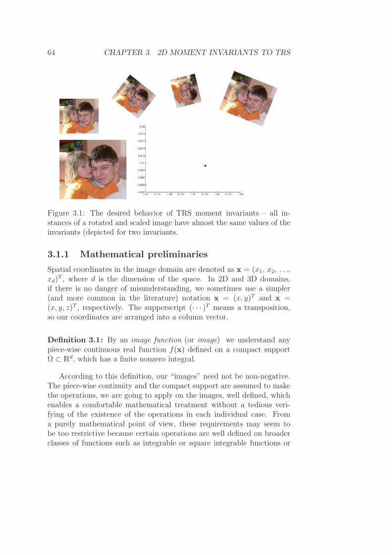
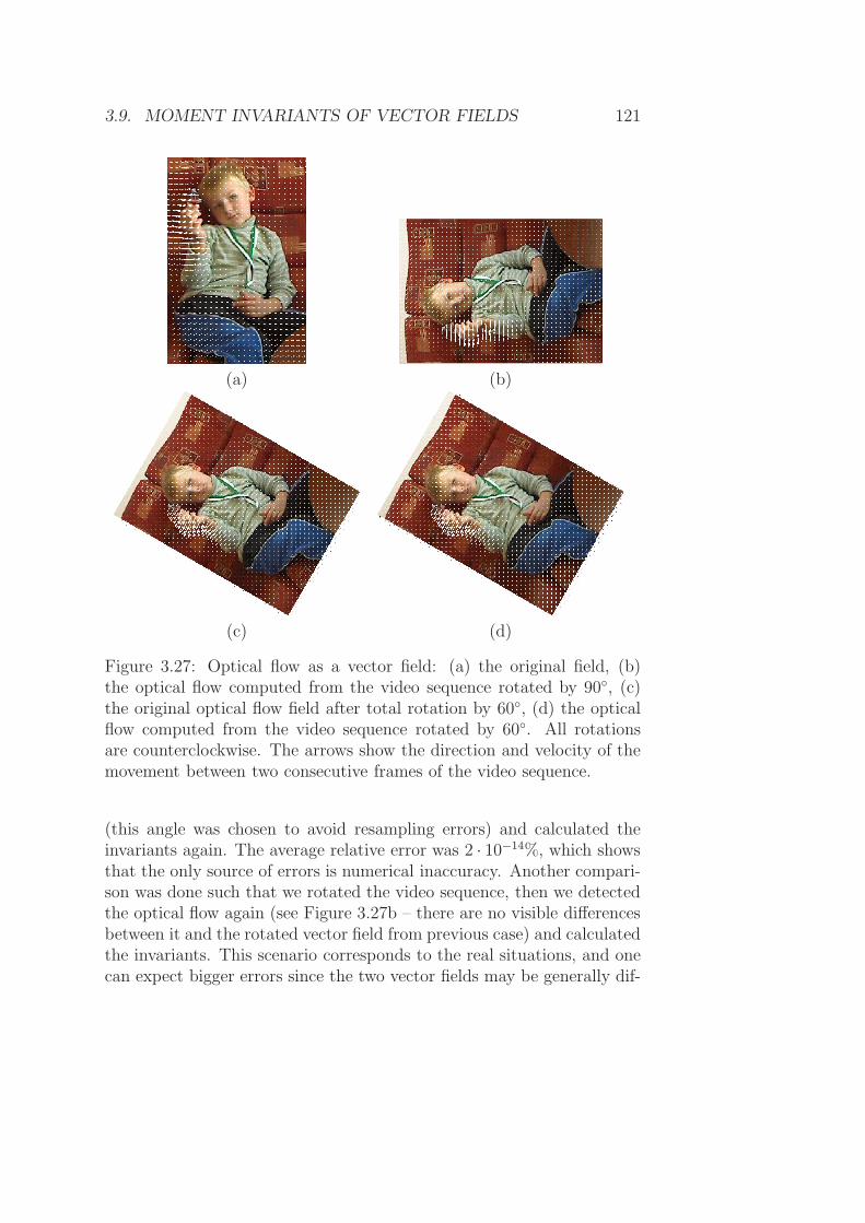
Figure 3.1: The desired behavior of TRS moment invariants – all in-stances of a rotated and scaled image have almost the same values of theinvariants (depicted for two invariants.

3.1.1 Mathematical preliminaries

Spatial coordinates in the image domain are denoted as x = (x1, x2, . . .,xd)

T , where d is the dimension of the space. In 2D and 3D domains,if there is no danger of misunderstanding, we sometimes use a simpler(and more common in the literature) notation x = (x, y)T and x =(x, y, z)T , respectively. The supperscript (· · · )T means a transposition,so our coordinates are arranged into a column vector.

Definition 3.1: By an image function (or image) we understand anypiece-wise continuous real function f(x) defined on a compact supportΩ ⊂ Rd, which has a finite nonzero integral.

According to this definition, our “images” need not be non-negative.The piece-wise continuity and the compact support are assumed to makethe operations, we are going to apply on the images, well defined, whichenables a comfortable mathematical treatment without a tedious veri-fying of the existence of the operations in each individual case. Froma purely mathematical point of view, these requirements may seem tobe too restrictive because certain operations are well defined on broaderclasses of functions such as integrable or square integrable functions or

3.1. INTRODUCTION 65

infinitely supported functions of fast decay. However, these nuances makeabsolutely no difference from a practical point of view when working withdigital images. The non-zero integral is required because its value willbe frequently used as a normalization factor1.

If the image is mathematically described by the image function, wesometimes speak about the continuous representation. Although thecontinuous representation may not reflect certain properties of digitalimages, such as sampling and quantization errors, we will adopt the con-tinuous formalism because of its mathematical transparency and sim-plicity. If the discrete character of the image is substantial (such as, forinstance, in chapter 8 where we explain numerical algorithms for momentcomputations), we will work with a discrete representation of the imagein a form of a finite-extent 2D matrix f = (fij) or 3D matrix f = (fijk),which is supposed to be obtained from the continuous representationf(x) by sampling and quantization.

The image function from Definition 3.1 represents monochromaticimages (sometimes also called graylevel or scalar images). If f hasonly two possible values (which are usually encoded as 0 and 1), wespeak about a binary image. Color images and vector-valued images arerepresented as a vector image function, each component of which satisfiesDefinition 3.1.

Convolution is an operation between two image functions2, the resultof which is another image function defined as

(f ∗ g)(x) =

∫

Rd

f(t)g(x− t)dt . (3.1)

Fourier transformation (FT) of image function f is defined as

F(f)(u) ≡ F (u) =

∫

Rd

e−2πiuxf(x)dx , (3.2)

where i is the imaginary unit, the components of u are spatial frequencies,and ux = u1x1 + . . . + udxd means scalar product3. Note that F(f)

1If we released this assumption, the invariants still could be constructed providedthat at least one moment is non-zero.

2Note that the convolution is not a point-wise operation between the functionvalues, so the notation f(x) ∗ g(x), commonly used in many engineering textbooks, ismisleading and mathematically incorrect.

3A more correct notation of the scalar product is uTx; we drop the superscript T

for simplicity.


always exists thanks to the integrability of f , and its support cannotbe bounded4. Fourier transformation is invertible through the inverseFourier transformation (IFT)

F−1(F )(x) =

∫

Rd

e2πiuxF (u)du = f(x) . (3.3)

We recall two important properties of FT, which we employ in thisbook. The first one, also known as the Fourier shift theorem, tells thatthe FT of a translated image function equals the FT of the original upto a phase shift

F(f(x− t))(u) = e−2πiutF(f(x))(u) . (3.4)

The second property, known as the convolution theorem, shows why FTis so useful in signal processing – it transfers the convolution into a point-wise multiplication in the frequency domain

F(f ∗ g)(u) = F (u)G(u) . (3.5)

3.1.2 Moments

Moments are scalar real or complex-valued features which have beenused to characterize a given function. From the mathematical pointof view, moments are “projections5” of function f onto a polynomialbasis (similarly, Fourier transformation is a projection onto a basis of theharmonic functions).

Definition 3.2: Let πp(x) be a d-variable polynomial basis of thespace of image functions defined on Ω and let p = (p1, . . . , pd) be amulti-index of non-negative integers which show the highest power of therespective variables in πp(x). Then the general moment M

(f)p of image

f is defined as

M (f)p =

∫

Ω

πp(x)f(x)dx . (3.6)

4More precisely, F(f) cannot vanish on any open subset of Rd.5The moments in general are not the coordinates of f in the given basis in the

algebraic sense. That is true for orthogonal bases only.


The number |p| =∑d

k=1 pk is called the order of the moment. We omitthe superscript (f) whenever possible without confusion.

Depending on the polynomial basis πp(x), we recognize varioussystems of moments. The most common choice is a standard power basisπp(x) = xp which leads to geometric moments

m(f)p =

∫

Ω

xpf(x)dx . (3.7)

In the literature, one can find various extensions of Definition 3.2.Some authors allow non-polynomial bases (more precisely, they allowbasis functions which are products of a polynomial and some other –usually harmonic – functions) and/or include various scalar factors andweighting functions in the integrand. Some other authors even totallyreplaced the polynomial basis by some other basis but still call such fea-tures moments – we can find wavelet moments [1] and step-like moments[2], where wavelets and step-wise functions are used in a combinationwith harmonic functions instead of the polynomials. These modificationsbroadened the notion of moments but have not brought any principle dif-ferences in moment usage.

3.1.3 Geometric moments in 2D

In case of 2D images, the choice of the standard power basis πpq(x, y) =xpyq yields 2D geometric moments

mpq =

∞∫

−∞

∞∫

−∞

xpyqf(x, y)dxdy. (3.8)

Geometric moments have been widely used in statistics for descriptionof the shape of a probability density function and in classic rigid-bodymechanics to measure the mass distribution of a body. Geometric mo-ments of low orders have an intuitive meaning – m00 is a “mass” of theimage (on binary images, m00 is an area of the object), m10/m00 andm01/m00 define the center of gravity or centroid of the image. Second-order moments m20 and m02 describe the “distribution of mass” of theimage with respect to the coordinate axes. In mechanics, they are called


the moments of inertia. Another popular mechanical quantity, the ra-dius of gyration with respect to an axis, can be also expressed in termsof moments as

√m20/m00 and

√m02/m00, respectively.

If the image is considered to be a joint probability density function(PDF) of two random variables (i.e., its values are non-negative and nor-malized such that m00 = 1), then the horizontal and vertical projectionsof the image are the 1D marginal densities, and m10 and m01 are themean values of the variables. In case of zero means, m20 and m02 aretheir variances, and m11 is a covariance between them. In this way,the second-order moments define the principal axes of the image. Aswill be seen later, the second-order geometric moments can be used tofind the normalized position of the image. In statistics, two higher-ordermoment characteristics of a probability density function have been com-monly used – the skewness and the kurtosis. These terms are mostlyused for 1D marginal densities only. Skewness of the horizontal marginaldensity is defined as m30/

√m3

20 and that of the vertical marginal distri-

bution as m03/√m3

02. The skewness measures the deviation of the PDFfrom symmetry. If the PDF is symmetric with respect to the mean (i.e.,to the origin in this case), then the corresponding skewness equals zero.The kurtosis measures the “peakedness” of the probability density func-tion and is again defined separately for each marginal distribution – thehorizontal kurtosis as m40/m

220 and the vertical kurtosis as m04/m

202.

Characterization of the image by means of the geometric moments iscomplete and unambiguous in the following sense. For any image func-tion, its geometric moments of all orders do exist and are finite. The im-age function can be exactly reconstructed from the set of all its moments(this assertion is known as the uniqueness theorem and holds thanks tothe Weirstrass theorem on infinitely accurate polynomial approximationof continuous functions)6.

Geometric moments of function f are closely related to its Fouriertransformation. If we expand the kernel of the Fourier transformatione−2πi(ux+vy) into a power series, we realize that the geometric momentsform Taylor coefficients of F

F (u, v) =∞∑

p=0

∞∑

q=0

(−2πi)p+q

p!q!mpqu

pvq .

6A more general moment problem is well known in statistics: can a given sequencebe a set of moments of some compactly supported function? The answer is yes if thesequence is completely monotonic.


This link between the geometric moments and Fourier transformationis employed in many tasks, for instance in image reconstruction frommoments as we will see in detail in Chapter 7.

3.1.4 Other moments

Geometric moments are very attractive thanks to the formal simplicityof the basis functions. This is why many theoretical considerations aboutmoment invariants have been based on them. On the other hand, theyhave also certain disadvantages. One of them is their complicated trans-formation under rotation. This has led to introducing a class of circularmoments, which change under rotation in a simple way and allow todesign rotation invariants systematically, as we will show later in thischapter for the 2D case and in chapter 4 for the 3D case.

Another drawback of the geometric moments are their poor numeri-cal properties when working in a discrete domain. Standard powers arenearly dependent both for small and large values of the exponent andincrease rapidly in range as the order increases. This leads to correlatedgeometric moments and to the need for high computational precision.Using lower precision results in unreliable computation of geometric mo-ments. This has led several authors to employing orthogonal (OG) mo-ments, that is, moments the basis polynomials of which are orthogonalon Ω.

In theory, all polynomial bases of the same degree are equivalentbecause they generate the same space of functions. Any moment withrespect to a certain basis can be expressed in terms of moments withrespect to any other basis. From this point of view, OG moments ofany type are equivalent to geometric moments. However, a significantdifference appears when considering stability and other computationalissues. OG moments have the advantage of requiring lower computingprecision because we can evaluate them using recurrent relations, withoutexpressing them in terms of the standard powers. OG moments arereviewed in chapter 7.


3.2 TRS invariants from geometric moments

Translation, rotation, and scaling in 2D is a four-parameter transfor-mation, which can be described in a matrix form as

x′ = sRαx+ t,

where t is a translation vector, s is a positive scaling factor (note thathere we consider uniform scaling only, that is, s is the same both inhorizontal and vertical directions), and Rα is a rotation matrix by theangle α

Rα =

(cosα − sinαsinα cosα

).

Note that the TRS transformations actually form a group because

R0 = I,

RαRβ = Rα+β

andR−1

α = R−α = RTα .

3.2.1 Invariants to translation

Geometric moments are not invariant to translation. If f is shifted byvector t = (a, b)T , then its geometric moments change as

m′

pq =

∞∫

−∞

∞∫

−∞

xpyqf(x− a, y − b)dxdy =

=

∞∫

−∞

∞∫

−∞

(x+ a)p(y + b)qf(x, y)dxdy =

=

p∑

k=0

q∑

j=0

(p

k

)(q

j

)akbjmp−k,q−j.

(3.9)

Invariance to translation can be achieved simply by seemingly shiftingthe object into a certain well-defined position before the moments arecalculated. The best way is to use its centroid – if we shift the objectsuch that its centroid coincides with the origin of the coordinate system,then all the moments are translation invariants. This is equivalent to

3.2. TRS INVARIANTS FROM GEOMETRIC MOMENTS 71

keeping the object fixed and shifting the polynomial basis into the objectcentroid7. We obtain so-called central geometric moments

µpq =

∞∫

−∞

∞∫

−∞

(x− xc)p(y − yc)

qf(x, y)dxdy, (3.10)

where

xc = m10/m00, yc = m01/m00

are the coordinates of the object centroid. Note that it always holdsµ10 = µ01 = 0 and µ00 = m00. Translation invariance of the centralmoments is straightforward.

The central moments can be expressed in terms of geometric momentsas

µpq =

p∑

k=0

q∑

j=0

(p

k

)(q

j

)(−1)k+jxk

cyjcmp−k,q−j.

Although this relation has little importance for theoretic consideration,it is sometimes used when we want to calculate the central moments bymeans of some fast algorithm for geometric moments computation.

3.2.2 Invariants to uniform scaling

Scaling invariance is obtained by a proper normalization of each moment.To find a normalization factor, let us first look at how the moment ischanged under image scaling8 by a factor s

µ′

pq =

∞∫

−∞

∞∫

−∞

(x− xc)p(y − yc)

qf(x/s, y/s)dxdy = (3.11)

=

∞∫

−∞

∞∫

−∞

sp(x− xc)psq(y − yc)

qf(x, y)s2dxdy = sp+q+2µpq.(3.12)

7We recall that the use of the centralized coordinates is a common way of reachingtranslation invariance also in case of many other than moment-based features.

8There is a difference between scaling the image and scaling the coordinates –upscaling the image is the same as downscaling the coordinates and vice versa, thescaling factors are inverse. However, for the purpose of deriving invariants, it doesnot matter which particular scaling we consider.


In particular,µ′

00 = s2µ00.

In principle, any moment can be used as a normalizing factor providedthat it is non-zero for all images in the experiment. Since low-ordermoments are more stable to noise and easier to calculate, we normalizemost often by a proper power of µ00

νpq =µpq

µw00

. (3.13)

To eliminate the scaling parameter s, the power must be set as

w =p+ q

2+ 1. (3.14)

The moment νpq is called the normalized central geometric moment9 andis invariant to uniform scaling:

ν ′

pq =µ′

pq

(µ′

00)w=

sp+q+2µpq

(s2µ00)w= νpq .

The moment that has been used for scaling normalization can nolonger be used for recognition because the value of the correspondingnormalized moment is always one (in the above normalization, ν00 = 1).If we want to keep the zero-order moment valid, we have to normalize byanother moment. Such kind of scaling normalization is used very rarely;probably the only meaningful normalization is by (µ20 + µ02)

w/2.

3.2.3 Invariants to non-uniform scaling

Non-uniform scaling is a transformation beyond the TRS frameworkthat maps a unit square onto a rectangle. It is defined as

x′ = ax,

y′ = by,

where a 6= b are positive scaling factors. Invariants to non-uniform scalingare sometimes called aspect-ratio invariants.

9This normalization was proposed already in Hu’s paper [3], but the exponent wasstated incorrectly as w = p+q+1

2. Many authors adopted this error, and some other

authors introduced a new one claiming w = [p+q

2] + 1, where [.] denotes an integer

part.


Figure 3.2: Numerical test of the normalized moment ν20. Computer-generated scaling of the test image ranged form s = 0.2 to s = 3. Toshow robustness, each image was corrupted by additive Gaussian whitenoise. Signal-to-noise ratio (SNR) ranged from 50 (low noise) to 10(heavy noise). Horizontal axes: scaling factor s and SNR, respectively.Vertical axis – relative deviation (in %) between ν20 of the original andthat of the scaled and noisy image. The test proves the invariance of ν20and illustrates its high robustness to noise.

Geometric central moments change under non-uniform scaling simplyas

µ′

pq =

∞∫

−∞

∞∫

−∞

ap(x− xc)pbq(y − yc)

qf(x, y)ab dx dy = ap+1bq+1µpq .


To eliminate the scaling factors a and b, we need at least two normalizingmoments. When using for instance µ00 and µ20, we get the invariants

Apq =µpq

µα00µ

β20

,

where

α =3q − p

2+ 1

and

β =p− q

2.

One can derive many different invariants to non-uniform scaling. Forinstance, Pan and Keane [4] proposed more “symmetric” normalizationby three moments µ00, µ20 and µ02, which leads to

Spq =µ(p+q+2)/200

µ(p+1)/220 · µ

(q+1)/202

· µpq.

Invariance to non-uniform scaling cannot be combined in a simple waywith rotation invariance. The reason is that rotation and non-uniformscaling are not closed operations. When applied repeatedly, they gener-ate an affine group of transformations, which implies that if we want tohave invariance to non-uniform scaling and rotation, we must use affineinvariants (they will be introduced in the chapter 5). There is no trans-formation group “between” the TRS and affine groups and, consequently,no special set of invariants “between” the TRS, and affine moment in-variants may exist. This is why the invariants to non-uniform scalingdescribed above are of only little importance in practical applications,and we presented them here merely for illustration.

3.2.4 Traditional invariants to rotation

Rotation moment invariants were firstly introduced in 1962 by Hu [3],who employed the results of the theory of algebraic invariants and derived


Figure 3.3: Numerical test of the aspect-ratio invariant A22. Computer-generated scaling of the test image ranged form 0.5 to 2 in both directionsindependently. Horizontal axes: scaling factors a and b, respectively.Vertical axis – relative deviation (in %) between A22 of the original andthat of the scaled image. The test illustrates the invariance of A22. Higherrelative errors for low scaling factors and typical jagged surface of thegraph are the consequences of the image resampling.

his seven famous invariants to an in-plane rotation around the origin

φ1 = m20 +m02,

φ2 = (m20 −m02)2 + 4m2

11,

φ3 = (m30 − 3m12)2 + (3m21 −m03)

2,

φ4 = (m30 +m12)2 + (m21 +m03)

2, (3.15)

φ5 = (m30 − 3m12)(m30 +m12)((m30 +m12)2 − 3(m21 +m03)

2) +

(3m21 −m03)(m21 +m03)(3(m30 +m12)2 − (m21 +m03)

2),

φ6 = (m20 −m02)((m30 +m12)2 − (m21 +m03)

2) +

4m11(m30 +m12)(m21 +m03),

φ7 = (3m21 −m03)(m30 +m12)((m30 +m12)2 − 3(m21 +m03)

2)−

(m30 − 3m12)(m21 +m03)(3(m30 +m12)2 − (m21 +m03)

2).


If we replace geometric moments by central or normalized moments inthese relations, we obtain invariants not only to rotation but also totranslation and/or scaling, which at the same time ensures invariance torotation around an arbitrary point. Hu’s derivation was rather compli-cated, and that is why only these seven invariants were derived explicitlyand no hint how to derive invariants from higher-order moments wasgiven in [3]. However, once we have the formulae, the proof of rotationinvariance is easy. Let us demonstrate it for φ1 and φ2.

The second-order moments after rotation by angle α can be expressedas

µ′

20 = cos2 α · µ20 + sin2 α · µ02 − sin 2α · µ11

µ′

02 = sin2 α · µ20 + cos2 α · µ02 + sin 2α · µ11

µ′

11 =1

2sin 2α · (µ20 − µ02) + cos 2α · µ11.

Thus,φ′

1 = µ′

20 + µ′

02 = (sin2 α + cos2 α)(µ20 + µ02) = φ1

and similarly for φ′

2, applying the formula cos 2α = cos2 α− sin2 α. ⊓⊔Although Hu’s invariants suffer from the limited recognition power,

mutual dependence, and the restriction to the second- and third-ordermoments only, they have become classics, and, despite of their drawbacks,they have found numerous successful applications in various areas. Themajor weakness of Hu’s theory is that it does not provide for a possibilityof any generalization. By means of it, we could not derive invariants fromhigher-order moments. To illustrate that, let us consider how a generalmoment is changed under rotation:

m′

pq =

∞∫

−∞

∞∫

−∞

(x cosα− y sinα)p(x sinα + y cosα)qf(x, y)dxdy =

=

∞∫

−∞

∞∫

−∞

p∑

k=0

q∑

j=0

(p

k

)(q

j

)xk+jyp+q−k−j(−1)p−k(cosα)q+k−j(sinα)p−k+j

f(x, y)dxdy =

=

p∑

k=0

q∑

j=0

(−1)p−k

(p

k

)(q

j

)(cosα)q+k−j(sinα)p−k+jmk+j,p+q−k−j .

(3.16)This is a rather complicated expression from which the rotation parame-ter α cannot be easily eliminated. An attempt was proposed by Jin and

3.3. ROTATION INVARIANTS USING CIRCULAR MOMENTS 77

Tianxu [5], but compared to the approach described in the sequel it isdifficult and not very transparent.

In the next section, we present a general approach to deriving rotationinvariants, which uses circular moments.

3.3 Rotation invariants using circular mo-

ments

After Hu, various approaches to the theoretical derivation of moment-based rotation invariants, which would not suffer from a limitation to loworders, have been published. Although nowadays the key idea seems tobe bright and straightforward, its first versions appeared in the literatureonly two decades after Hu’s paper.

The key idea is to replace the cartesian coordinates (x, y) by (central-ized) polar coordinates (r, θ)

x = r cos θ r =√

x2 + y2

y = r sin θ θ = arctan(y/x)(3.17)

In the polar coordinates, the rotation is a translation in the angularargument. To eliminate the impact of this translation, we were inspiredby the Fourier shift theorem – if the basis functions in angular directionwere harmonics, the translation would result just in a phase shift of themoment values, which would be easy to eliminate. This brilliant generalidea led to the birth of a family of so-called circular moments10. Thecircular moments have the form

Cpq =

∞∫

0

2π∫

0

Rpq(r)eiξ(p,q)θf(r, θ)rdθdr (3.18)

where Rpq(r) is a radial univariate polynomial and ξ(p, q) is a function(usually a very simple one) of the indices. Complex, Zernike, pseudo-Zernike, Fourier-Mellin, radial Chebyshev, and many other moments areparticular cases of the circular moments.

Under coordinate rotation by angle α (which is equivalent to image

10They are sometimes referred to as radial or radial-circular moments.


rotation by −α), the circular moment is changed as

C ′

pq =

∞∫

0

2π∫

0

Rpq(r)eiξ(p,q)θf(r, θ + α)rdθdr =

=

∞∫

0

2π∫

0

Rpq(r)eiξ(p,q)(θ−α)f(r, θ)rdθdr =

= e−iξ(p,q)αCpq .

(3.19)

To eliminate the parameter α, we can take the moment magnitude |Cpq|(note that the circular moments are generally complex-valued even iff(x, y) is real) or apply some more sophisticated method to reach thephase cancelation (such a method of course depends on the particularfunction ξ(p, q)).

The above idea can be traced in several papers, which basically dif-fer from each other by the choice of the radial polynomials Rpq(r), thefunction ξ(p, q), and by the method by which α is eliminated.

Teague [6] and Wallin [7] proposed to use Zernike moments, which area special case of circular moments, and to take their magnitudes. Li [8]used Fourier-Mellin moments to derive invariants up to the order 9, Wong[9] used complex monomials up to the fifth order that originate from thetheory of algebraic invariants. Mostafa and Psaltis [10] introduced theidea to use complex moments for deriving invariants, but they focusedon the evaluation of the invariants rather than on constructing higher-order systems. This approach was later followed by Flusser [11, 12], whoproposed a general theory of constructing rotation moment invariants.His theory, presented in the next section, is based on the complex mo-ments. It is formally simple and transparent, allows deriving invariantsof any orders, and enables studying mutual dependence/independence ofthe invariants in a readable way. The usage of the complex moments isnot essential; this theory can be easily modified for other circular mo-ments as was for instance demonstrated by Derrode and Ghorbel [13]for Fourier-Mellin moments and Yang et al. [14] for Gaussian-Hermitemoments.

3.4. ROTATION INVARIANTS FROM COMPLEX MOMENTS 79

3.4 Rotation invariants from complex mo-

ments

In this section, we present a general method of deriving complete and in-dependent sets of rotation invariants of any orders. This method employscomplex moments of the image.

3.4.1 Complex moments

The complex moment cpq is obtained when we choose the polynomialbasis of complex monomials πpq(x, y) = (x+ iy)p(x− iy)q

cpq =

∞∫

−∞

∞∫

−∞

(x+ iy)p(x− iy)qf(x, y)dxdy. (3.20)

It follows from the definition that only the indices p ≥ q are independentand worth considering because cpq = c∗qp (the asterisk denotes complexconjugate).

Complex moments carry the same amount of information as the ge-ometric moments of the same order. Each complex moment can be ex-pressed in terms of geometric moments as

cpq =

p∑

k=0

q∑

j=0

(p

k

)(q

j

)(−1)q−j · ip+q−k−j ·mk+j,p+q−k−j (3.21)

and vice versa11

mpq =1

2p+qiq

p∑

k=0

q∑

j=0

(p

k

)(q

j

)(−1)q−j · ck+j,p+q−k−j. (3.22)

We can also see the link between the complex moments and Fouriertransformation. The complex moments are almost (up to a multiplica-tive constant) the Taylor coefficients of the Fourier transformation ofF(f)(u+ v, i(u− v)). If we denote U = u+ v and V = i(u− v), then we

11While the proof of (3.21) is straightforward, the proof of (3.22) requires first toexpress x and y as x = ((x + iy) + (x− iy))/2 and y = ((x+ iy)− (x− iy))/2i.


have

F(f)(U, V ) ≡∞∫

−∞

∞∫−∞

e−2πi(Ux+V y)f(x, y)dxdy =

=

∞∑

j=0

∞∑

k=0

(−2πi)j+k

j!k!cjku

jvk.(3.23)

When expressed in polar coordinates, the complex moments take theform

cpq =

∞∫

0

2π∫

0

rp+qei(p−q)θf(r, θ)rdθdr. (3.24)

Hence, the complex moments are special cases of the circular momentswith a choice of Rpq = rp+q and ξ(p, q) = p− q. The following lemma isa consequence of the rotation property of circular moments.

Lemma 3.3: Let f ′ be a rotated version (around the origin) of f , i. e.f ′(r, θ) = f(r, θ + α). Then

c′pq = e−i(p−q)α · cpq. (3.25)

3.4.2 Construction of rotation invariants

The simplest method proposed by many authors (see [15] for instance) isto use as invariants the moment magnitudes themselves. However, theydo not generate a complete set of invariants – by taking the magnitudesonly we miss many useful invariants. In the following theorem, phasecancelation is achieved by multiplication of appropriate moment powers.

Theorem 3.4: Let n ≥ 1, and let ki, pi ≥ 0, and qi ≥ 0 (i = 1, . . . , n)be arbitrary integers such that

n∑

i=1

ki(pi − qi) = 0.

Then

I =n∏

i=1

ckipiqi (3.26)

is invariant to rotation.


Proof: Let us consider rotation by angle α. Then

I ′ =n∏

i=1

c′kipiqi

=n∏

i=1

e−iki(pi−qi)α · ckipiqi = e−iα∑n

i=1ki(pi−qi) · I = I. ⊓⊔

According to Theorem 3.4, some simple examples of rotation invari-ants are c11, c20c02, c20c

212, and so on. Most invariants (3.26) are complex.

If real-valued features are required, we consider real and imaginary partsof each of them separately. To achieve also translation invariance, weuse central coordinates in the definition of the complex moments (3.20)and we discard all invariants containing c10 and c01. Scaling invariancecan be achieved by the same normalization as we used for the geometricmoments.

3.4.3 Construction of the basis

In this section, we will pay attention to the construction of a basis ofinvariants up to a given order. Theorem 3.4 allows us to construct aninfinite number of invariants for any order of moments, but only fewof them being mutually independent. By the term basis we intuitivelyunderstand the smallest set required to express all other invariants. Moreprecisely, the basis must be independent, which means that none of itselements can be expressed as a function of the other elements, and alsocomplete, meaning that any rotation invariant can be expressed by meansof the basis elements only.

The knowledge of the basis is a crucial point in all pattern recognitiontasks because the basis provides the same discriminative power as the setof all invariants and thus minimizes the computational cost. For instance,the set

c20c02, c221c02, c

212c20, c21c12, c

321c02c12

is a dependent set whose basis is c212c20, c21c12.To formalize these terms, we first introduce the following definitions.

Definition 3.5: Let k ≥ 1, let I = I1, . . . , Ik be a set of rotationinvariants. Let J be also a rotation invariant. J is said to be dependenton I if and only if there exists a function F of k variables such that

J = F (I1, . . . , Ik).

J is said to be independent on I otherwise.


Definition 3.6: Let k > 1 and let I = I1, . . . , Ik be a set of rotationinvariants. The set I is said to be dependent if and only if there existsk0 ≤ k such that Ik0 depends on I −· Ik0. The set I is said to beindependent otherwise.

According to this definition, c20c02, c220c

202, c

221c02, c21c12, c

321c02c12,

and c20c212, c02c

221 are examples of dependent invariant sets.

Definition 3.7: Let I be a set of rotation invariants, and let B be itssubset. B is called a complete subset if and only if any element of I −· Bdepends on B. The set B is a basis of I if and only if it is independentand complete.

Now we can formulate a fundamental theorem that tells us how toconstruct an invariant basis of a given order.

Theorem 3.8: Let us consider complex moments up to the order r ≥ 2.Let a set of rotation invariants B be constructed as follows:

B = Φ(p, q) ≡ cpqcp−qq0p0

|p ≥ q ∧ p+ q ≤ r,

where p0 and q0 are arbitrary indices such that p0 + q0 ≤ r, p0 − q0 = 1and cp0q0 6= 0 for all admissible images. Then B is a basis of all rotationinvariants12 created from the moments of any kind up to the order r.

Theorem 3.8 is very strong because it claims B is a basis of all possiblerotation moment invariants, not only of those constructed according to(3.26) and not only of those which are based on complex moments. Inother words, B provides at least the same discrimination power as anyother set of moment invariants up to the given order r ≥ 2 because anypossible invariant can be expressed in terms of B. (Note that this is atheoretical property; it may be violated in the discrete domain wheredifferent polynomials have different numerical properties.)Proof: Let us prove the independence of B first. Let us assume B isdependent, that is, there exists Φ(p, q) ∈ B, such that it depends on

12The correct notation should be B(p0, q0) because the basis depends on the choiceof p0 and q0; however, we drop these indexes for simplicity.


B −· Φ(p, q). As follows from the linear independence of the polyno-mials (x + iy)p(x − iy)q and, consequently, from independence of thecomplex moments themselves, it must hold that p = p0 and q = q0.That means, according to the above assumption, there exist invariantsΦ(p1, q1), . . . ,Φ(pn, qn) and Φ(s1, t1), . . . ,Φ(sm, tm) from B −· Φ(p0, q0)and positive integers k1, . . . , kn and ℓ1, . . . , ℓm such that

Φ(p0, q0) =

∏n1

i=1Φ(pi, qi)ki ·

∏ni=n1+1Φ

∗(pi, qi)ki

∏m1

i=1Φ(si, ti)ℓi ·

∏mi=m1+1Φ

∗(si, ti)ℓi. (3.27)

Substituting into (3.27) and grouping the factors cp0q0 and cq0p0 together,we get

Φ(p0, q0) =c∑n1

i=1ki(pi−qi)

q0p0 · c∑n

i=n1+1ki(qi−pi)

p0q0 ·∏n1

i=1 ckipiqi

·∏n

i=n1+1 ckiqipi

c∑m1

i=1ℓi(si−ti)

q0p0 · c∑m

i=m1+1ℓi(ti−si)

p0q0 ·∏m1

i=1 cℓisiti ·

∏mi=m1+1 c

ℓitisi

.

(3.28)Comparing the exponents of cp0q0 and cq0p0 on both sides, we get theconstraints

K1 =n1∑

i=1

ki(pi − qi)−m1∑

i=1

ℓi(si − ti) = 1 (3.29)

and

K2 =

n∑

i=n1+1

ki(qi − pi)−

m∑

i=m1+1

ℓi(ti − si) = 1. (3.30)

Since the rest of the right-hand side of eq. (3.28) must be equal to 1, andsince the moments themselves are mutually independent, the followingconstraints must be fulfilled for any index i:

n1 = m1, n = m, pi = si, qi = ti, ki = ℓi.

Introducing these constraints into (3.29) and (3.30), we get K1 = K2 = 0which is a contradiction.

To prove the completeness of B, it is sufficient to resolve the so-calledinverse problem, which means to recover all complex moments (and, con-sequently, all geometric moments) up to the order r when knowing theelements of B. Thus, the following nonlinear system of equations mustbe resolved for the cpq’s:


Φ(p0, q0) = cp0q0cq0p0,

Φ(0, 0) = c00,

Φ(1, 0) = c10cq0p0,

Φ(2, 0) = c20c2q0p0,

Φ(1, 1) = c11, (3.31)

Φ(3, 0) = c30c3q0p0

,

. . .

Φ(r, 0) = cr0crq0p0

,

Φ(r − 1, 1) = cr−1,1cr−2q0p0 ,

. . .

Since B is a set of rotation invariants, it does not reflect the actualorientation of the object. Thus, there is one degree of freedom whenrecovering the object moments that correspond to the choice of the objectorientation. Without loss of generality, we can choose such orientation inwhich cp0q0 is real and positive. As can be seen from eq. (3.25), if cp0q0 isnonzero then such orientation always exists. The first equation of (3.31)can be then immediately resolved for cp0q0:

cp0q0 =√

Φ(p0, q0).

Consequently, using the relationship cq0p0 = cp0q0, we obtain the solutions

cpq =Φ(p, q)

cp−qq0p0

andcpp = Φ(p, p)

for any p and q. Recovering the geometric moments is straightforwardfrom eq. (3.8). Since any polynomial is a linear combination of standardpowers xpyq, any moment (and any moment invariant) can be expressedas a function of geometric moments, which completes the proof. ⊓⊔

Theorem 3.8 allows us not only to create the basis but also to calculatethe number of its elements in advance. Let us denote it as |B|. If r isodd then

|B| =1

4(r + 1)(r + 3),


if r is even then

|B| =1

4(r + 2)2.

(These numbers refer to complex-valued invariants.) We can see that theauthors who used the moment magnitudes only actually lost about halfof the information containing in the basis B.

The basis defined in Theorem 3.8 is generally not unique. It dependson the particular choice of p0 and q0, which is very important. How shallwe select these indices in practice? On the one hand, we want to keep p0and q0 as small as possible because lower-order moments are less sensitiveto noise than the higher-order ones. On the other hand, the close-to-zerovalue of cp0q0 may cause numerical instability of the invariants. Thus, wepropose the following algorithm. We start with p0 = 2 and q0 = 1 andcheck if |cp0q0| exceeds a pre-defined threshold for all objects (in practicethis means for all given training samples or database elements). If thiscondition is met, we accept the choice; in the opposite case we increaseboth p0 and q0 by one and repeat the above procedure.

3.4.4 Basis of the invariants of the second and third

orders

In this section, we present a basis of the rotation invariants composed ofthe moments of the second and third orders, that is constructed accordingto Theorem 3.8 by choosing p0 = 2 and q0 = 1. The basis is

Φ(1, 1) = c11,

Φ(2, 1) = c21c12, (3.32)

Φ(2, 0) = c20c212,

Φ(3, 0) = c30c312.

In this case, the basis is determined unambiguously and contains sixreal-valued invariants. It is worth noting that formally, according toTheorem 3.8, the basis should contain also invariants Φ(0, 0) = c00 andΦ(1, 0) = c10c12. We did not include these two invariants in the basisbecause c00 = µ00 is in most recognition applications used for normal-ization to scaling, and c10 = m10 + im01 is used to achieve translationinvariance. Then Φ(0, 0) = 1 and Φ(1, 0) = 0 for any object and it is


useless to consider them. Numerical stability of Φ(2, 0) is illustrated inFigure 3.4.

Figure 3.4: Numerical test of the basic invariant Φ(2, 0). Computer-generated rotation of the test image ranged form 0 to 360 degrees. Toshow robustness, each image was corrupted by additive Gaussian whitenoise. Signal-to-noise ratio (SNR) ranged from 40 (low noise) to 10(heavy noise). Horizontal axes: rotation angle and SNR, respectively.Vertical axis – relative deviation (in %) between Re(Φ(2, 0)) of the orig-inal and that of the rotated and noisy image. The test proves the invari-ance of Re(Φ(2, 0)) and illustrates its high robustness to noise.


3.4.5 Relationship to the Hu invariants

In this section, we highlight the relationship between the Hu invariants(3.15) and the proposed invariants (3.32). We show the Hu invariants areincomplete and mutually dependent, which can explain some practicalproblems connected with their usage.

It can be seen that the Hu invariants are nothing but particular rep-resentatives of the general form (3.26)

φ1 = c11,

φ2 = c20c02,

φ3 = c30c03,

φ4 = c21c12, (3.33)

φ5 = Re(c30c312),

φ6 = Re(c20c212),

φ7 = Im(c30c312)

and that they can be expressed also in terms of the basis (3.32)

φ1 = Φ(1, 1)

φ2 =|Φ(2, 0)|2

Φ(2, 1)2

φ3 =|Φ(3, 0)|2

Φ(2, 1)3

φ4 = Φ(2, 1)

φ5 = Re(Φ(3, 0))

φ6 = Re(Φ(2, 0))

φ7 = Im(Φ(3, 0)).

Using (3.33), we can demonstrate the dependency of the Hu invariants.It holds

φ3 =φ25 + φ2

7

φ34

,

which means that either φ3 or φ4 is useless and can be excluded from theHu’s system without any loss of discrimination power.

Moreover, we show the Hu’s system is incomplete. Let us try torecover complex and geometric moments when knowing φ1, . . ., φ7 underthe same normalization constraint as in the previous case, i.e. c21 is


required to be real and positive. Complex moments c11, c21, c12, c30, andc03 can be recovered in a straightforward way:

c11 = φ1,

c21 = c12 =√

φ4,

Re(c30) = Re(c03) =φ5

c312,

Im(c30) = −Im(c03) =φ7

c312.

Unfortunately, c20 cannot be fully recovered. We have, for its real part,

Re(c20) =φ6

c212

but for its imaginary part we get

(Im(c20))2 = |c20|

2 − (Re(c20))2 = φ2 −

(φ6

c212

)2

.

There is no way of determining the sign of Im(c20). In terms of geometricmoments, it means the sign of m11 cannot be recovered.

The incompleteness of the Hu invariants implicates their lower dis-crimination power compared to the proposed invariants of the same order.Let us consider two objects f(x, y) and g(x, y), both in the normalizedcentral positions, having the same geometric moments up to the thirdorder except m11, for which m

(f)11 = −m

(g)11 . In the case of artificial data,

such object g(x, y) exists for any given f(x, y) and can be designed as

g(x, y) = (f(x, y) + f(−x, y) + f(x,−y)− f(−x,−y))/2, (3.34)

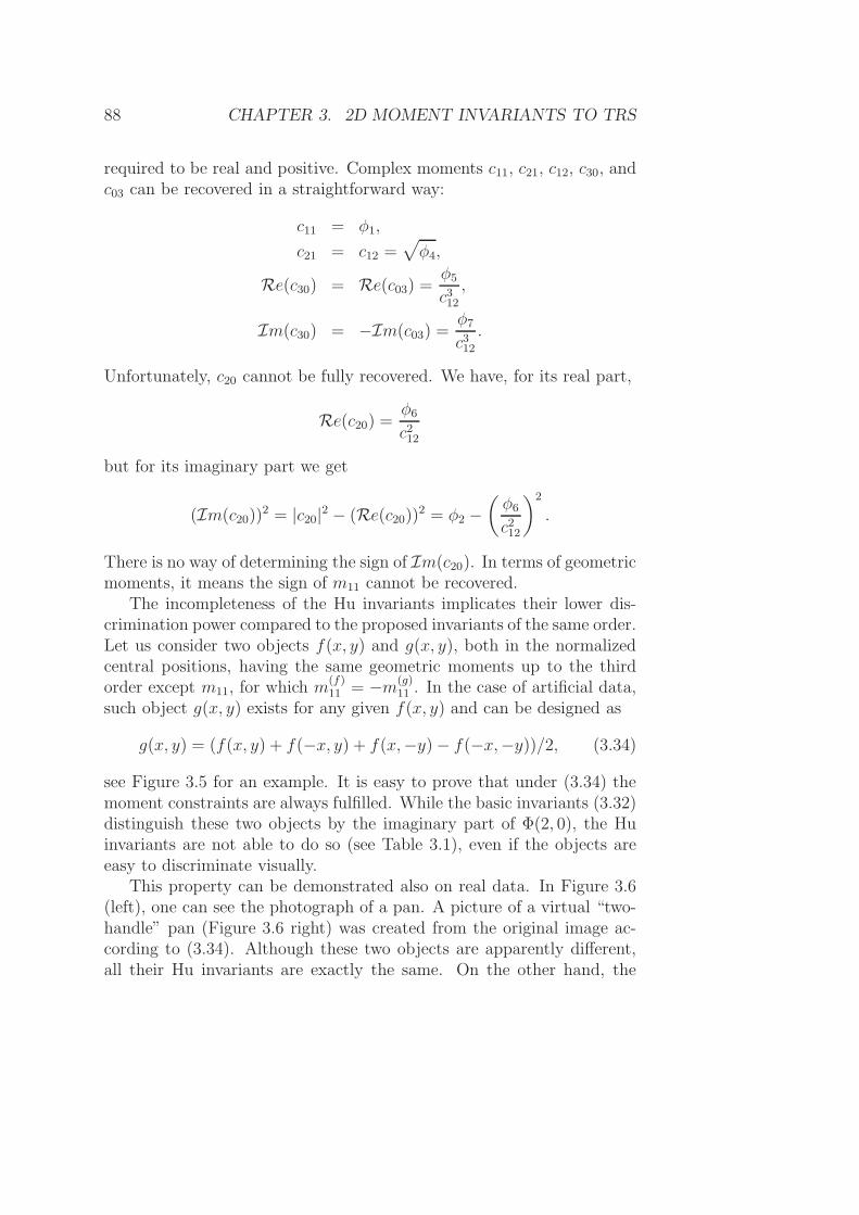
see Figure 3.5 for an example. It is easy to prove that under (3.34) themoment constraints are always fulfilled. While the basic invariants (3.32)distinguish these two objects by the imaginary part of Φ(2, 0), the Huinvariants are not able to do so (see Table 3.1), even if the objects areeasy to discriminate visually.

This property can be demonstrated also on real data. In Figure 3.6(left), one can see the photograph of a pan. A picture of a virtual “two-handle” pan (Figure 3.6 right) was created from the original image ac-cording to (3.34). Although these two objects are apparently different,all their Hu invariants are exactly the same. On the other hand, the


new invariant Φ(2, 0) distinguishes these two objects clearly thanks tothe opposite signs of its imaginary part.

This ambiguity cannot be avoided by a different choice of the normal-ization constraint when recovering the moments. Let us, for instance,consider another normalization constraint, which requires c20 to be realand positive. In terms of geometric moments, it corresponds to the re-quirement m11 = 0 and m20 > m02. Then, similarly to the previouscase, the signs of (m30+m12) and (m03+m21) cannot be unambiguouslydetermined.

(a) (b)

Figure 3.5: The smiles: (a) original and (b) another figure created fromthe original according to Eq. (3.34). For the values of the respectiveinvariants see Table 3.1.

(a) (b)

Figure 3.6: (a) Original image of a pan and (b) a virtual “two-handle”pan. These objects are distinguishable by the basic invariants but notby the Hu invariants.

It is worth noting that also other earlier sets of rotation invariants are


Table 3.1: The values of the Hu invariants and the basic invariants (3.32)of “The smiles” in Figure 3.5. The only invariant discriminating themis Im(Φ(2, 0)). (The values shown here were calculated after bringingFigure 3.5 into normalized central position c21 > 0 and nonlinearly scaledto the range from -10 to 10 for display.)

Hu Fig. 3.5(a) Fig. 3.5(b) Basic Fig. 3.5(a) Fig. 3.5(b)φ1 4.2032 4.2032 Φ(1, 1) 4.2032 4.2032φ2 1.7563 1.7563 Φ(2, 1) 6.5331 6.5331φ3 3.6395 3.6395 Re(Φ(2, 0)) 8.6576 8.6576φ4 6.5331 6.5331 Im(Φ(2, 0)) 7.6437 -7.6437

φ5 1.0074 1.0074 Re(Φ(3, 0)) 1.0074 1.0074φ6 8.6576 8.6576 Im(Φ(3, 0)) -6.9850 -6.9850φ7 -6.9850 -6.9850

dependent and/or incomplete. This was, however, not mentioned in theoriginal papers, partly because the authors did not pay attention to theseissues and partly because their methods did not allow them to find out thedependencies among the invariants in a systematic way. Li [8] publisheda set of invariants from moments up to the ninth order. Unfortunately,his system includes the Hu invariants and therefore it also cannot be abasis. Jin and Tianxu [5] derived twelve invariants in explicit form butonly eight of them are independent. Wong [9] presented a set of sixteeninvariants from moments up to the third order and a set of “more thanforty-nine” invariants from moments up to the fourth order. It followsimmediately from Theorem 3.8 that the basis of the third-order invariantshas only six elements and the basis of the fourth-order invariants hasnine elements. Thus, most of the Wong’s invariants are dependent andof no practical significance. Even Mukundan’s monograph [16] presentsa dependent and incomplete set of twenty-two rotation invariants up tothe sixth order (see [16], p. 125). The construction of the invariants fromthe complex moments has resolved the independence and completenessissues in an elegant way.

3.5. PSEUDOINVARIANTS 91

3.5 Pseudoinvariants

In this section, we investigate the behavior of rotation invariants undermirror reflection of the image (see Figure 3.7). Since the mirror reflectionis not a special case of the TRS transformation, the rotation invariantsmay change when the image is mirrored. The mirror reflection can occurin some applications only, but it is useful to know how the rotationinvariants behave in that case. We show they cannot change arbitrarily.There are only two possibilities – a (real-valued) invariant can either stayconstant or change its sign. The invariants, which preserve their valueunder reflection are traditionally called true invariants while those thatchange the sign are called pseudoinvariants [6] or, misleadingly, skewinvariants [3]. Pseudoinvariants discriminate between mirrored imagesof the same object, which is useful in some applications but may beundesirable in other cases. We show which invariants from the basisintroduced in Theorem 3.8 are pseudoinvariants and which are the trueones.

Let us consider a basic invariant, and let us investigate its behaviorunder a reflection across an arbitrary line. Due to the rotation and shiftinvariance, we can limit ourselves to the reflection across the x-axis.

Let f(x, y) be a mirrored version of f(x, y), i.e. f(x, y) = f(x,−y).As follows from the definition,

cpq = cqp = c∗pq.

Thus, it holds for any basic invariant Φ(p, q)

Φ(p, q) = cpqcp−qq0p0 = c∗pq · (c

∗

q0p0)p−q = Φ∗(p, q).

This proves that the real parts of the basic invariants are true invariants.On the other hand, the imaginary parts of them change their signs underreflection and hence are pseudoinvariants. This brings a consequence forthe recognition of objects with axial symmetry. The pseudoinvariantscannot differentiate among any axially symmetric objects because theirvalues must always be zero.


Figure 3.7: The test image and its mirrored version. Basic invariants ofthe mirrored image are complex conjugates of those of the original.

3.6 Combined invariants to TRS and con-

trast

stretching

So far we have considered invariants to spatial transformations only.However, if the features used in a recognition system are calculated froma graylevel/color image and not just from a binary image, they shouldbe invariant also to various changes of intensity. These changes may becaused by the change of illumination conditions, by the camera setup, bythe influence of the environment, and by many other factors. In Chap-ter 6 we describe invariants to graylevel degradations caused by linearfiltering. In this section we consider contrast stretching only, which is a

3.6. COMBINED INVARIANTS TO TRS AND CONTRAST STRETCHING93

very simple graylevel transformation given as

f ′(x, y) = a · f(x, y),

where a is a positive stretching factor. This model approximately de-scribes the change of the illumination of the scene between two acquisi-tions (in case of digital images, this model may not be valid everywherebecause f ′(x, y) might overflow the 8-bit intensity range at some places,but we ignore this issue here for simplicity). The invariants to contraststretching in connection with Hu’s rotation invariants were firstly pro-posed by Maitra [17] and later improved by Hupkens [18]. Here we willdemonstrate how to include the invariance to contrast stretching into theTRS invariants described earlier in this chapter.

Since µ′

pq = a · µpq and c′pq = a · cpq, pure contrast (and transla-tion) invariance and can be achieved simply by normalizing each centralor complex moment by µ00. Now consider a contrast stretching and arotation together. It holds for any basic invariant Φ(p, q)

Φ′(p, q) = ap−q+1Φ(p, q),

and it is sufficient to use the normalization

Φ(p, q)

µp−q+100

.

This approach unfortunately cannot be further extended to scaling. Ifµ00 has been used for normalization to contrast, it cannot be at the sametime used for scaling normalization. We have to normalize by some otherinvariant, preferably by c11 for the sake of simplicity.

Let cpq be defined as follows

cpq =cpqµ

p+q

2−1

00

cp+q

2

11

.

Then cpq is both contrast and scaling normalized moment, which can beused for constructing rotation invariants in a usual way as

Ψ(p, q) = cpqcq0p0p−q.

This is possible because c11 itself is a rotation invariant. Hence, Ψ(p, q)is a combined TRS and contrast invariant. Note that Ψ(1, 1) = 1 for anyobject due to the normalization.


Figure 3.8: Numerical test of the contrast and TRS invariant Ψ(2, 0)for p0 = 2 and q0 = 1. Computer-generated scaling of the test imageranged from s = 0.2 to s = 3, and the contrast stretching factor rangedfrom a = 0.1 to a = 2. Horizontal axes: scaling factor s and contraststretching factor a, respectively. Vertical axis – relative deviation (in %)between Re(Ψ(2, 0)) of the original and that of the scaled and stretchedimage. The test proves the invariance of Re(Ψ(2, 0)) with respect toboth factors. However, for down-scaling with s = 0.2 and s = 0.3, theresampling effect leads to higher relative errors.

3.7. ROTATION INVARIANTS OF SYMMETRIC OBJECTS 95

3.7 Rotation invariants for recognition of

symmetric objects

In many applied tasks, we want to classify man-made objects or naturalshapes from their silhouettes (i.e., from binary images) only. In mostcases such shapes have some kind of symmetry. Different classes mayhave the same symmetry, which makes the task even more difficult. Whilehumans can use the symmetry as a cue that helps them to recognizeobjects, moment-based classifiers suffer from the fact that some momentsof symmetric shapes are zero and corresponding invariants do not provideany discrimination power. This is why we must pay attention to thesesituations and why it is necessary to design special invariants for eachtype of symmetry [19].

For example, all odd-order moments (geometric as well as complex)of a centrosymmetric object are identically equal to zero. If an objectis circularly symmetric, all its complex moments, whose indices are dif-ferent, vanish. Thus, Theorem 3.8 either cannot be applied at all, ormany rotation invariants might be useless. Let us imagine an illustrativeexample. We want to recognize three shapes – a square, a cross, and acircle – independently of their orientation. Because of the symmetry, allcomplex moments of the second and third orders except c11 are zero. Ifthe shapes are appropriately scaled, c11 can be the same for all of them.Consequently, neither the Hu invariants nor the basic invariants fromTheorem 3.8 provide any discrimination power, even if the shapes canbe readily recognized visually. Appropriate invariants in this case wouldbe c22, c40c04, c51c04, c33, c80c

204, c62c04, c44, etc. The above simple example

shows the necessity of having different systems of invariants for objectswith different types of symmetry.

We have only two types of object symmetry which are relevant toconsider in this context13 – N-fold rotation symmetry (N -FRS) and N-fold dihedral symmetry (N -FDS).

Object f is said to have N -FRS if it is “rotationally periodic”, that isif it repeats itself when it rotates around the origin (which is supposed tobe shifted into the object centroid) by αj = 2πj/N for all j = 1, . . . , N .

13In the theory of point groups in 2D, it is well known that there exist only cyclicgroups CN , dihedral groups DN , and translational symmetry groups which are irrel-evant here.


(a) (b) (c)

(d) (e)

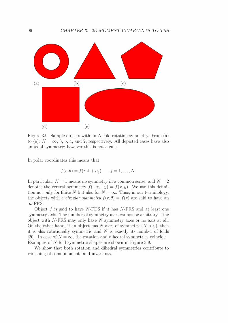
Figure 3.9: Sample objects with an N -fold rotation symmetry. From (a)to (e): N = ∞, 3, 5, 4, and 2, respectively. All depicted cases have alsoan axial symmetry; however this is not a rule.

In polar coordinates this means that

f(r, θ) = f(r, θ + αj) j = 1, . . . , N.

In particular, N = 1 means no symmetry in a common sense, and N = 2denotes the central symmetry f(−x,−y) = f(x, y). We use this defini-tion not only for finite N but also for N = ∞. Thus, in our terminology,the objects with a circular symmetry f(r, θ) = f(r) are said to have an∞-FRS.

Object f is said to have N -FDS if it has N -FRS and at least onesymmetry axis. The number of symmetry axes cannot be arbitrary – theobject with N -FRS may only have N symmetry axes or no axis at all.On the other hand, if an object has N axes of symmetry (N > 0), thenit is also rotationally symmetric and N is exactly its number of folds[20]. In case of N = ∞, the rotation and dihedral symmetries coincide.Examples of N -fold symmetric shapes are shown in Figure 3.9.

We show that both rotation and dihedral symmetries contribute tovanishing of some moments and invariants.

3.7. INVARIANTS FOR RECOGNITION OF SYMMETRIC OBJECTS97

Lemma 3.9: If f(x, y) has an N -fold rotation symmetry (N finite) andif (p− q)/N is not an integer, then cpq = 0.

Proof: Let us rotate f around the origin by 2π/N . Due to its symmetry,the rotated object f ′ must be the same as the original. In particular, itmust hold c′pq = cpq for any p and q. On the other hand, it follows fromeq. (3.25) that

c′pq = e−2πi(p−q)/N · cpq.

Since (p − q)/N is assumed not to be an integer, this equation can befulfilled only if cpq = 0.14 ⊓⊔

Lemma 3.9a: If f(x, y) has ∞-fold rotation symmetry and if p 6= q,then cpq = 0.

Proof: Let us rotate f around the origin by an arbitrary angle α. Therotated version f ′ must be the same as the original for any α, and, con-sequently, its moments cannot change under rotation. Eq. (3.25) implies

c′pq = e−i(p−q)α · cpq.

Since p 6= q and α may be arbitrary, this equation can be fulfilled only ifcpq = 0. ⊓⊔

The above lemma shows that the matrix of the complex momentsCij = ci−1,j−1 of an N -fold symmetric object always has a specific struc-ture – it is a sparse multidiagonal (and of course Hermitian) matrix withnon-zero entries on the major diagonal and on the minor diagonals withthe equidistant spacing of N (see Figure 3.10).

The other elements are always zero, so we have to avoid their usageas the factors in the invariants. In order to derive invariants for recog-nition of objects with N -fold rotation symmetry, Theorem 3.8 can begeneralized in the following way.

Theorem 3.10: Let N ≥ 1 be a finite integer. Let us consider complexmoments up to the order r ≥ N . Let a set of rotation invariants BN beconstructed as follows:

BN = ΦN(p, q) ≡ cpqckq0p0

|p ≥ q∧p+q ≤ r∧k ≡ (p−q)/N is an integer,

14This lemma can be generalized for any circular moment; the moment vanishes ifξ(p, q)/N is not an integer.


Figure 3.10: The matrix of the complex moments of an N -fold symmet-ric object. The gray elements are always zero. The distance betweenneighboring non-zero diagonals is N .

where p0 and q0 are arbitrary indices such that p0 + q0 ≤ r, p0 − q0 =N , and cp0q0 6= 0 for all admissible objects. Then BN is a basis of allnon-trivial rotation invariants for objects with N -FRS, created from themoments up to the order r.

Proof: Rotation invariance of all elements of BN follows immediatelyfrom Theorem 3.4. The independence and completeness of BN can beproven exactly in the same way as in Theorem 3.8, when only non-zeromoments are recovered. ⊓⊔

If 2 ≤ r < N , no such cp0q0 exists, and the basis is

BN = cpp | p ≤ r/2.

For N = 1, which means no rotation symmetry, Theorem 3.10 is reducedexactly to Theorem 3.8; B1 = B and Φ1(p, q) = Φ(p, q). The followingmodification of Theorem 3.10 deals with the case of N = ∞.

Theorem 3.10a: Let us consider complex moments up to the orderr ≥ 2. Then the basis B∞ of all non-trivial rotation invariants for objects


with ∞-FRS isB∞ = cpp | p ≤ r/2.

The proof of Theorem 3.10a follows immediately from Theorem 3.4 andLemma 3.9a. Note that matrix C is diagonal for N = ∞.

Theorems 3.10 and 3.10a have several interesting consequences. Someof them are summarized in the following lemma.

Lemma 3.11: Let us denote all rotation invariants that can be ex-pressed by means of elements of basis B as 〈B〉. Then it holds for anyorder r

1. If M and N are finite and L is their least common multiple, then

〈BM〉 ∩ 〈BN〉 = 〈BL〉.

In particular, if M/N is an integer, then 〈BM〉 ⊂ 〈BN〉.

2.∞⋂

N=1

〈BN〉 = 〈B∞〉.

3. If N is finite, the number of elements of BN is

|BN | =

[r/N ]∑

j=0

[r − jN + 2

2

],

where [a] means an integer part of a. For N = ∞ it holds

|B∞| =

[r + 2

2

].

From the last point of Lemma 3.11 we can see that the higher thenumber of folds, the fewer non-trivial invariants exist. The number ofthem ranges from about r2/4 for non-symmetric objects to about r/2 forcircularly symmetric ones.

If an object has an N -FDS, then its moment matrix has the samemultidiagonal structure, but the axial symmetry introduces additionaldependence between the real and imaginary parts of each moment. The


actual relationship between them depends on the orientation of the sym-metry axis. If we, however, consider the basic rotation invariants fromTheorem 3.10, the dependence on the axis orientation disappears; theimaginary part of each invariant is zero (we already showed this prop-erty in Section 3.5).

In practical pattern recognition experiments, the number of folds Nmay not be known a priori. In that case we can apply a fold detector (see[21, 22, 23, 24] for sample algorithms15 detecting the number of folds) toall elements of the training set before we choose an appropriate system ofmoment invariants. In case of equal fold numbers of all classes, the properinvariants can be chosen directly according to Theorem 3.10 or 3.10a.Usually we start selecting from the lowest orders, and the appropriatenumber of the invariants is determined such that they should provide asufficient discriminability of the training set.

If there are shape classes with different numbers of folds, the previoustheory does not provide a universal solution to this problem. If we wantto find such invariants which are non-trivial on all classes, we cannotsimply choose one of the fold numbers detected as the appropriate Nfor constructing invariant basis according to Theorem 3.10 (althoughone could intuitively expect the highest number of folds to be a goodchoice, this is not that case). A more sophisticated choice is to takethe least common multiple of all finite fold numbers and then to applyTheorem 3.10. Unfortunately, taking the least common multiple oftenleads to high-order instable invariants. This is why in practice one mayprefer to decompose the problem into two steps – first, pre-classificationinto “groups of classes” according to the number of folds is performed,and then final classification is done by means of moment invariants, whichare defined separately within each group. This decomposition can beperformed explicitly in a separate pre-classification stage or implicitlyduring the classification. The word “implicitly” here means that thenumber of folds of an unknown object is not explicitly tested, however,at the beginning we must test the numbers of folds in the training set.We explain the latter version.

15These fold detectors look for the angular periodicity of the image, either directlyby calculating the circular autocorrelation function and searching for its peaks orby investigating circular Fourier transformation and looking for dominant frequency.Alternatively, some methods estimate the fold number directly from the zero valuesof certain complex moments or other circular moments. Such approach may howeverbe misleading in some cases because the moment values could be small even if theobject is not symmetric.


Let us have C classes altogether such that Ck classes have Nk foldsof symmetry; k = 1, . . ., K; N1 > N2 > . . .NK . The set of properinvariants can be chosen as follows. Starting from the highest symmetry,we iteratively select those invariants providing (jointly with the invariantsthat have been already selected) a sufficient discriminability between theclasses with the fold numbers NF and higher, but which may equal zerofor some (or all) other classes. Note that for some F the algorithm neednot to select any invariant because the discriminability can be assuredby the invariants selected previously or because CF = 1.

In order to illustrate the importance of a careful choice of the invari-ants in pattern recognition tasks, we carried out the following experi-mental studies.

3.7.1 Logo recognition

In the first experiment, we tested the capability of recognizing objectshaving the same number of folds, particularly N = 3. As a test setwe used three logos of major companies (Mercedes-Benz, Mitsubishi,and Fischer) and two commonly used symbols (“recycling” and “woolenproduct”). All logos were downloaded from the respective web-sites, re-sampled to 128 × 128 pixels and binarized. We decided to use logos asthe test objects because most logos have a certain degree of symmetry.This experiment is also relevant to the state of the art because severalcommercial logo/trademark recognition systems reported in the litera-ture [25, 26, 27, 28] used rotation moment invariants as features, and allof them face the problem of symmetry.

Figure 3.11: The test logos (from left to right): Mercedes-Benz, Mit-subishi, Recycling, Fischer, and Woolen product.

As can be seen in Figure 3.11, all our test logos have three-fold rota-tion symmetry. Each logo was rotated ten times by randomly generatedangles. Since the spatial resolution of the images was relatively high, thesampling effect was insignificant. Moment invariants from Theorem 3.10


0 0.5 1 1.5 2 2.5 3

x 10−9

0

1

2

3

4

5

6

7x 10

−12

c30

c03

Re(

c 41c 03

)

Figure 3.12: The logo positions in the space of two invariants c30c03and Re(c41c03) showing good discrimination power. The symbols: –Mercedes-Benz, – Mitsubishi, – Recycling, – Fischer, and –Woolen product. Each logo was randomly rotated ten times.

(N = 3, p0 = 3, and q0 = 0) provide an excellent discrimination powereven if only the two simplest ones have been used (see Figure 3.12), whilethe invariants from Theorem 3.8 are not able to distinguish the logos atall (see Figure 3.13).

3.7.2 Recognition of shapes with different fold num-

bers

In the second experiment, we used nine simple binary patterns with var-ious numbers of folds: capitals F and L (N = 1), rectangle and diamond(N = 2), equilateral triangle and tripod (N = 3), cross (N = 4), andcircle and ring (N = ∞) (see Figure 3.14). As in the previous case, eachpattern was rotated ten times by random angles.

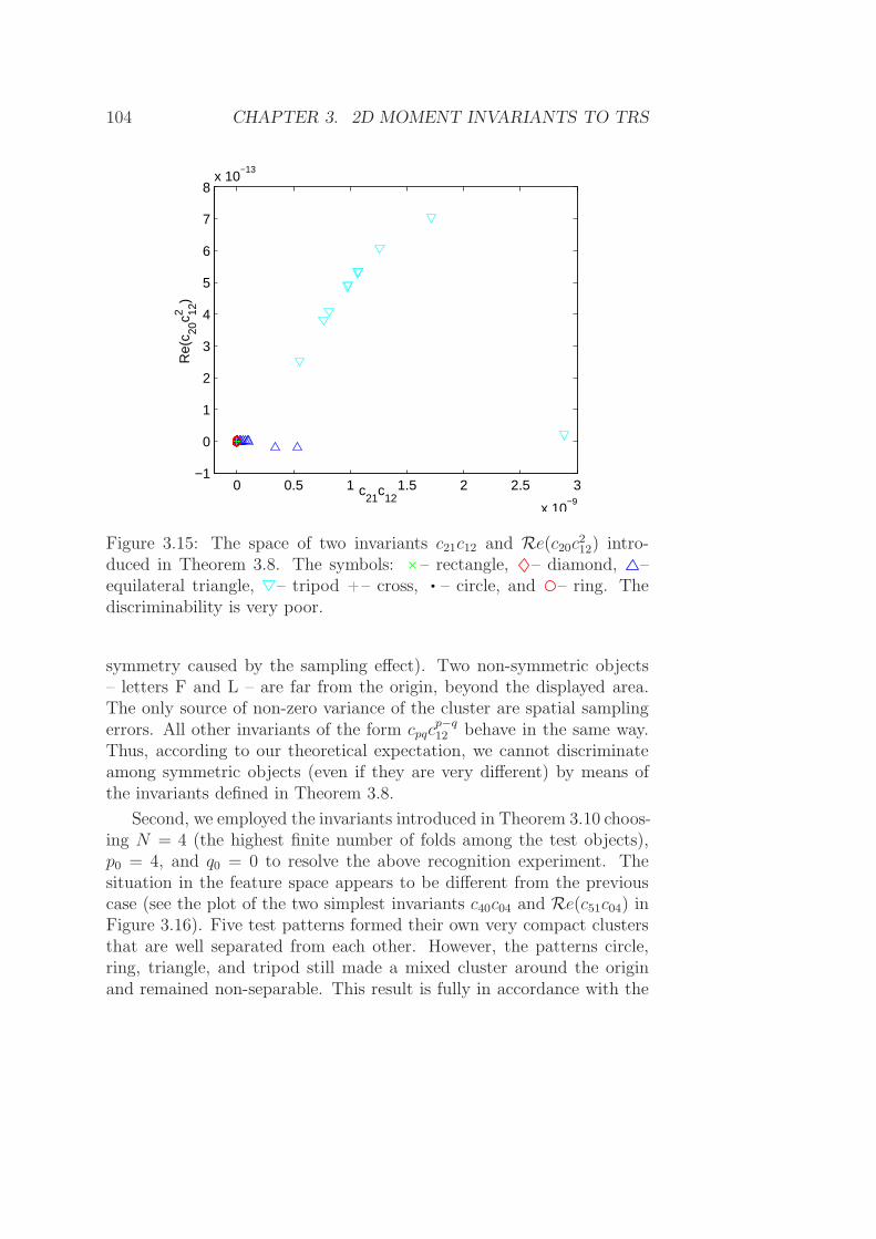
First, we applied rotation invariants according to Theorem 3.8 choos-ing p0 = 2 and q0 = 1. The positions of our test patterns in the featurespace are plotted in Figure 3.15. Although only a 2-D subspace showing


0 5 10 15 20

x 10−13

−1

0

1

2

3

4

5x 10

−17

c21

c12

Re(

c 20c 122

)

Figure 3.13: The logo positions in the space of two invariants c21c12 andRe(c20c

212) introduced in Theorem 3.8. These invariants have no discrim-

ination power with respect to this logo set. The symbols: – Mercedes-Benz, – Mitsubishi, – Recycling, – Fischer, and – Woolen prod-uct.

Figure 3.14: The test patterns: capital L, rectangle, equilateral triangle,circle, capital F, diamond, tripod, cross, and ring.

the invariants c21c12 and Re(c20c212) is visualized there, we can easily ob-

serve that the patterns form a single dense cluster around the origin (theonly exception is the tripod, which is slightly biased because of its non-


0 0.5 1 1.5 2 2.5 3

x 10−9

−1

0

1

2

3

4

5

6

7

8x 10

−13

c21

c12

Re(

c 20c 122

)

Figure 3.15: The space of two invariants c21c12 and Re(c20c212) intro-

duced in Theorem 3.8. The symbols: – rectangle, – diamond, –equilateral triangle, – tripod – cross, – circle, and – ring. Thediscriminability is very poor.

symmetry caused by the sampling effect). Two non-symmetric objects– letters F and L – are far from the origin, beyond the displayed area.The only source of non-zero variance of the cluster are spatial samplingerrors. All other invariants of the form cpqc

p−q12 behave in the same way.

Thus, according to our theoretical expectation, we cannot discriminateamong symmetric objects (even if they are very different) by means ofthe invariants defined in Theorem 3.8.

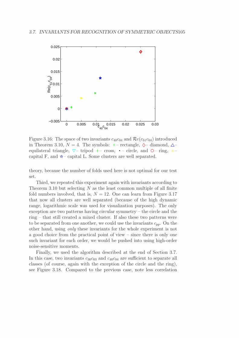
Second, we employed the invariants introduced in Theorem 3.10 choos-ing N = 4 (the highest finite number of folds among the test objects),p0 = 4, and q0 = 0 to resolve the above recognition experiment. Thesituation in the feature space appears to be different from the previouscase (see the plot of the two simplest invariants c40c04 and Re(c51c04) inFigure 3.16). Five test patterns formed their own very compact clustersthat are well separated from each other. However, the patterns circle,ring, triangle, and tripod still made a mixed cluster around the originand remained non-separable. This result is fully in accordance with the


0 0.005 0.01 0.015 0.02 0.025 0.03−0.005

0

0.005

0.01

0.015

0.02

0.025

c40

c04

Re(

c 51c 04

)

Figure 3.16: The space of two invariants c40c04 andRe(c51c04) introducedin Theorem 3.10, N = 4. The symbols: – rectangle, – diamond, –equilateral triangle, – tripod – cross, – circle, and – ring, –capital F, and – capital L. Some clusters are well separated.

theory, because the number of folds used here is not optimal for our testset.

Third, we repeated this experiment again with invariants according toTheorem 3.10 but selecting N as the least common multiple of all finitefold numbers involved, that is, N = 12. One can learn from Figure 3.17that now all clusters are well separated (because of the high dynamicrange, logarithmic scale was used for visualization purposes). The onlyexception are two patterns having circular symmetry – the circle and thering – that still created a mixed cluster. If also these two patterns wereto be separated from one another, we could use the invariants cpp. On theother hand, using only these invariants for the whole experiment is nota good choice from the practical point of view – since there is only onesuch invariant for each order, we would be pushed into using high-ordernoise-sensitive moments.

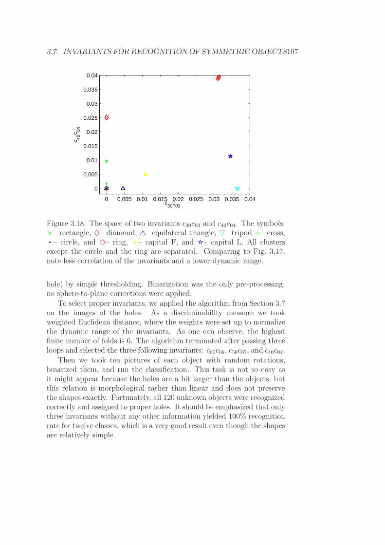
Finally, we used the algorithm described at the end of Section 3.7.In this case, two invariants c30c03 and c40c04 are sufficient to separate allclasses (of course, again with the exception of the circle and the ring),see Figure 3.18. Compared to the previous case, note less correlation


10−20

10−15

10−10

10−5

100

10−20

10−15

10−10

10−5

100

c12,0

c0,12

Re(

c 13,1

c 0,12

)

Figure 3.17: The space of two invariants c12,0c0,12 and Re(c13,1c0,12) intro-duced in Theorem 3.10, N = 12 (logarithmic scale). The symbols: –rectangle, – diamond, – equilateral triangle, – tripod – cross, –circle, and – ring, – capital F, and – capital L. All clusters exceptthe circle and the ring are separated.

of the invariants, their higher robustness, and lower dynamic range. Onthe other hand, neither c30c03 nor c40c04 provide enough discriminationpower when used individually while the twelfth-order invariants are ableto distinguish all classes.

3.7.3 Experiment with a baby toy

We demonstrate the performance of invariants in an object matchingtask. We used a popular baby toy (see Figure 3.19) that is also com-monly used in testing computer vision algorithms and robotic systems.The toy consists of a hollow sphere with twelve holes and of twelve ob-jects of various shapes. Each object matches up with just one particularhole. The baby (or the algorithm) is supposed to assign the objects tothe corresponding holes and insert them into the sphere. The baby canemploy both the color and shape information; however, in our experimentwe completely disregarded the colors to make the task more challenging.

First, we binarized the pictures of the holes (one picture per each


0 0.005 0.01 0.015 0.02 0.025 0.03 0.035 0.04

0

0.005

0.01

0.015

0.02

0.025

0.03

0.035

0.04

c30

c03

c 40c 04

Figure 3.18: The space of two invariants c30c03 and c40c04. The symbols:– rectangle, – diamond, – equilateral triangle, – tripod – cross,– circle, and – ring, – capital F, and – capital L. All clusters

except the circle and the ring are separated. Comparing to Fig. 3.17,note less correlation of the invariants and a lower dynamic range.

hole) by simple thresholding. Binarization was the only pre-processing;no sphere-to-plane corrections were applied.

To select proper invariants, we applied the algorithm from Section 3.7on the images of the holes. As a discriminability measure we tookweighted Euclidean distance, where the weights were set up to normalizethe dynamic range of the invariants. As one can observe, the highestfinite number of folds is 6. The algorithm terminated after passing threeloops and selected the three following invariants: c60c06, c50c05, and c40c04.

Then we took ten pictures of each object with random rotations,binarized them, and run the classification. This task is not so easy asit might appear because the holes are a bit larger than the objects, butthis relation is morphological rather than linear and does not preservethe shapes exactly. Fortunately, all 120 unknown objects were recognizedcorrectly and assigned to proper holes. It should be emphasized that onlythree invariants without any other information yielded 100% recognitionrate for twelve classes, which is a very good result even though the shapesare relatively simple.


Figure 3.19: The toy set used in the experiment.

We repeated the classification once again with invariants constructedaccording to Theorem 3.8 setting p0 = 2, q0 = 1. Only three objects hav-ing 1-fold symmetry were recognized correctly, the others were classifiedrandomly.

3.8 Rotation invariants via image normal-

ization

The TRS invariants can also be derived in another way than by means ofTheorem 3.8. This alternative method called image normalization firstbrings the image into some “standard” or “canonical” position, which isdefined by setting certain image moments to pre-defined values (usually

3.8. ROTATION INVARIANTS VIA IMAGE NORMALIZATION 109

0 or 1). Then the moments of the normalized image (except those thathave been used to define the normalization constraints) can be used asTRS invariants of the original image. It should be noted that no actualgeometric transformation and resampling of the image is required; themoments of the normalized image can be calculated directly from theoriginal image by means of normalization constraints.

While normalization to translation and scaling is trivial by settingm′

10 = m′

01 = 0 and m′

00 = 1, there are many possibilities of defining thenormalization constraints to rotation. The traditional one known as theprincipal axismethod [3] requires for the normalized image the constraintµ′

11 = 0.16 It leads to diagonalization of the second-order moment matrix

M =

(µ20 µ11

µ11 µ02

). (3.35)

It is well-known that any symmetric matrix can be diagonalized on thebasis of its (orthogonal) eigenvectors. After finding the eigenvalues of M(they are guaranteed to be real) by solving

|M− λI| = 0,

we obtain the diagonal form

M′ = GTMG =

(λ1 00 λ2

)=

(µ′

20 00 µ′

02

),

where G is an orthogonal matrix composed of the eigenvectors of M. Itis easy to show that we obtain for the eigenvalues of M

µ′

20 ≡ λ1 = ((µ20 + µ02) +√(µ20 − µ02)2 + 4µ2

11)/2,

µ′

02 ≡ λ2 = ((µ20 + µ02)−√

(µ20 − µ02)2 + 4µ211)/2,

and that the angle between the first eigenvector and the x-axis, which isactually the normalization angle, is 17

α =1

2· arctan

(2µ11

µ20 − µ02

).

16The reader may notice a clear analogy with the principal component analysis.17Some authors define the normalization angle with an opposite sign. Both ways

are, however, equivalent – we may “rotate” either the image or the coordinates.


Provided that λ1 > λ2, there are four different normalization angleswhich all make µ′

11 = 0: α, α + π/2, α + π, and α + 3π/2. To removethe ambiguity between “horizontal” and “vertical” position, we imposethe constraint µ′

20 > µ′

02. Removing the “left-right” ambiguity can beachieved by introducing an additional constraint µ′

30 > 0 (provided thatµ′

30 is nonzero; a higher-order constraint must be used otherwise).If λ1 = λ2, then any nonzero vector is an eigenvector of M, and

the principal axis method would yield infinitely many solutions. This ispossible only if µ11 = 0 and µ20 = µ02; the principal axis normalizationcannot be used in that case.

Now each moment of the normalized image µ′

pq is a rotation invariantof the original image. For the second-order moments, we can see clearcorrespondence with the Hu invariants

µ′

20 = (φ1 +√φ2)/2,

µ′

02 = (φ1 −√

φ2)/2.

The principal axis normalization is linked with a notion of the ref-erence ellipse (see Figure 3.20). There exist two concepts in the litera-ture18. The first one, which is suitable namely for binary images, requiresthe ellipse to have a unit intensity. The other one, which is more generaland more convenient for graylevel images, requires a constant-intensityellipse, but its intensity may be arbitrary. The former approach allows toconstraining the first- and the second-order moments of the ellipse suchthat they equal the moments of the image, but the zero-order momentof the ellipse is generally different from that of the image.

After the principal axis normalization, the reference ellipse is in axialposition, and we have the following constraints for its moments,

µ(e)11 = 0,

µ(e)20 ≡

πa3b

4= µ′

20,

µ(e)02 ≡

πab3

4= µ′

02,

where a and b are the length of the major and minor semiaxis, respec-tively. By the last two constraints, a and b are unambiguously deter-mined.

18Whenever one uses the reference ellipse, it must be specified which definition hasbeen applied.


If we apply the latter definition of the reference ellipse, the constraintsalso contain the ellipse intensity ℓ, which allows us to constraint also thezero-order moment

µ(e)00 ≡ πℓab = µ′

00,

µ(e)11 = 0,

µ(e)20 ≡

πℓa3b

4= µ′

20,

µ(e)02 ≡

πℓab3

4= µ′

02.

These constraints allow an unambiguous calculation of a, b, and ℓ.All images having the same second-order moments have identical ref-

erence ellipses. This can also be understood from the opposite side –knowing the second-order image moments, we can reconstruct the refer-ence ellipse only, without any finer image details.

Figure 3.20: Principal axis normalization to rotation – an object in thenormalized position along with its reference ellipse superimposed.

Mostafa and Psaltis [29] proposed a general normalization scheme bymeans of the complex moments. Their normalization constraint requiresone complex moment cst, where s 6= t, of the image to be real and positive(we could of course use any other well-defined orientation, but this onewas chosen for simplicity). As follows from Eq. (3.25), this is alwayspossible to achieve provided that cst 6= 0. Then the constraint leads tothe normalization angle

α =1

s− t· arctan

(Im(cst)

Re(cst)

). (3.36)


Figure 3.21: Ambiguity of the principal axis normalization. These fourpositions of the object satisfy µ′

11 = 0. Additional constraints µ′

20 > µ′

02

and µ′

30 > 0 make the normalization unique.

There exist exactly s− t distinct angles satisfying (3.36), see Figure 3.22.This normalization is unambiguous only if s − t = 1. For s − t > 1,additional constraints are required to remove the ambiguity. If we chooses = 2 and t = 0, the constraint (3.36) brings us back to the principalaxis normalization.

The selection of the normalizing moment cst is a critical step, and inpractice it must be done very carefully. If we calculated the normaliza-tion angle with an error, this error would propagate and would affect allinvariants. Even a very small error in the normalizing angle can influencesome invariants significantly. The non-zero constraint is easy to check ina continuous domain, but in a discrete case some moments that are infact zero due to the object symmetry may appear in certain positions ofthe object as nonzero because of the sampling effect. We have to identifysuch moments and avoid their usage in the normalization. At the sametime, we want to keep the moment order s+ t as low as possible in order


Figure 3.22: An example of the ambiguity of the normalization by com-plex moments. In all these six positions, c′60 is real and positive as re-quired.

to make the normalization robust.

The normalizing moment can be found as follows. We sort all complexmoments (except those that were already used for translation and scalingnormalization) up to the given order r according to the index differencep−q and those moments with the same index differences we sort accordingto their order. We obtain an ordered sequence c21, c32, c43, . . ., c20, c31,c42, c53, . . ., etc. The first nonzero moment in this sequence is then usedfor normalization. To test if the moment is nonzero, we compare its valuewith a user-defined threshold. The choice of the threshold must reflect themagnitudes of the moments in question, and, especially when consideringhigh r, it may be useful to define different thresholds for different momentorders. If all moments in the sequence are zero, we consider the objectcircularly symmetric, and no normalization is necessary.

One can, of course, use another ordering scheme when looking forthe normalizing moment. An alternative is to sort the moments in theother way round – first according to their orders and the moments ofthe same order according to the index differences. Both methods have


certain advantages and drawbacks. For non-symmetric objects there isno difference because we always choose c21. For symmetric and close-to-symmetric objects, when we sort the moments according to their ordersfirst, then the order of the chosen moment is kept as low as possible.This is a favorable property because low-order moments are more robustto noise than higher-order ones. On the other hand, one can find ob-jects where this approach fails. Sorting moments according to the indexdifference first generally leads to a higher-order normalization constraintthat is numerically less stable, but from the theoretical point of view thisworks for any object.

There have been many discussions on the advantages and drawbacksof both approaches – moment invariants and image normalization. Herewe show that from the theoretical point of view they are fully equivalentand that the normalizing moment cst and the basic moment cp0q0 playvery similar roles.

Let us consider the basis of the rotation invariants designed accordingto Theorem 3.8. We can apply the Mostafa and Psaltis normalizationmethod with cst = cp0q0 . Since each Φ(p, q) is a rotation invariant, itholds

Φ(p, q) = c′pqc′p−qq0p0

,

where c′pq denotes the moments of the normalized image. Consequently,since c′q0p0 is real and positive, we get

Φ(p, q) = c′pq|cp0q0|p−q. (3.37)

Eq. (3.37) shows that there is a one-to-one mapping between momentinvariants Φ(p, q) of the original image and complex moments c′pq of thenormalized image. An analogous result can be obtained for symmet-ric objects and the invariants from Theorem 3.10. Thus, normalizationapproach and invariant-based approach are equivalent on the theoreticallevel. Computational issues in particular applications might be, however,different.

3.9 Moment invariants of vector fields

A vector-valued image f(x) can be viewed as a set of m scalar imagesf(x) = (f1(x), . . . , fm(x))

T . Depending on its character, there may bevarious relationships among individual components fk, which influencethe behavior of f under spatial transformations and hence influence the

3.9. MOMENT INVARIANTS OF VECTOR FIELDS 115

design of the invariants. Examples of vector-valued images are conven-tional color/multispectral images and vector fields. The former are notvery difficult to handle because their components (even if they are usuallycorrelated) can be treated as independent graylevel images, which allowsus to apply the rotation invariants derived earlier in this chapter sepa-rately to each component. However, the vector fields behave differentlyand require a different treatment.

A 2D vector field is a vector-valued image f(x) with d = m = 2.Typical examples of vector fields are gradient fields, particle velocityfields, optical flow fields, fluid flow fields, and others, see Figures 3.23,3.24, 3.25 and 3.27. A common feature is that at each point (x, y), thevalue of f(x, y) shows the orientation and the magnitude of certain vector.

Figure 3.23: Turbulence in a fluid (the colors show the local velocity ofthe flow; the direction is not displayed).

If a 2D vector-valued image f(x) is rotated, we have to distinguishfour kinds of rotation. Inner rotation is a traditional rotation knownfrom scalar images

f ′(x) = f(R−αx).

Outer rotation does not affect the spatial coordinates but acts on the


Figure 3.24: Image gradient as a vector field. For visualization purposes,the field is depicted by arrows on a sparse grid and laid over the originalLena image.

Figure 3.25: The wind velocity forecast for the Czech Republic (courtesyof the Czech Hydrometeorological Institute, the numerical model Aladin).The longer dash is constant part of the wind, the shorter dash expressesperpendicular squalls. The figure actually represents two vector fields.


vector values onlyf ′(x) = Rαf(x).

It appears for instance in color images when the color space rotates butthe picture itself does not move. Total rotation is a combination of bothinner and outer rotations of the same rotation matrices

f ′(x) = Rαf(R−αx).

Finally, the most general independent total rotation is a total rotation forwhich the outer and inner rotation matrices are different

f ′(x) = Rαf(Rβx).

Let us illustrate these terms in Figure 3.26 for α = 22.5. In the caseof the inner rotation, each arrow sustains its direction, but it is rotatedaround the image center to the new position. In the outer rotation, eacharrow sustains its position, but its direction is rotated by 22.5. In thetotal rotation, each arrow is rotated around the image center to the newposition, and its direction is also rotated by the same angle.

Traditional spatial-domain rotation of a color image is inner rotationsince the colors do not change. Rotation of a vector field is typicallya total rotation because if a vector field is rotated in the coordinatespace, then its values must be rotated accordingly such that the vectordirections are preserved relative to the image content. An independenttotal rotation may appear when spatially rotating a color image at thesame time that we independently rotate the color space.

Analogously to various kinds of rotations, we recognize inner scalingf ′(x) = f(x/s), outer scaling f ′(x) = sf(x), total scaling f ′(x) = sf(x/s),and independent total scaling f ′(x) = s1f(x/s2). For vector fields, typicalscaling in practice is the total scaling. We could also analogously definean inner, outer, total, and independent total translations, but it does notmake much sense in this context because the translation of a vector fieldin practice is always the inner one.

Although some vector field images may arrive as the results of im-age or video processing, such as gradients and optical flow images, wemeet vector field images more often in visualization of fluid flow and ofparticle motion. These images may come from the solution of Navier-Stokes equations as well as from real measurements and may show, forinstance, flowing water in a pipe or an air flow around an aircraft wingor around a coachwork. For engineers and designers, it is very important


(a) (b)

(c) (d)

Figure 3.26: Various rotations of a vector field: (a) the original vectorfield, (b) the inner rotation, (c) the outer rotation, (d) the total rotation.The graylevels corresponds to the vector sizes.

to identify singularities in the flow such as sinks and vortexes becausethey increase the friction, decrease the speed of the medium, and conse-quently increase the power and cost which is necessary to transport themedium through the pipe or the object through the air or water. Search-ing for the singularities is a typical template matching problem – we havea database of template singularities, and we look for these patterns in


the vector field. Since the orientation of the template is unknown andirrelevant, we cannot just correlate the templates but need invariants tototal rotation.

This problem was addressed for the first time by Schlemmer et al.[30] who realized that the invariants from complex moments can be usedhere in a similar way as for the graylevel images. If d = m = 2, we cantreat the vector field as a field of complex numbers

f(x, y) = f1(x, y) + if2(x, y)

which allows us to use the standard definition of complex moments. Itholds

c(f)pq = c(f1)pq + ic(f2)pq .

Unlike the moments of a scalar image, it holds for the vector fields mo-ments in general

c(f)pq 6= c(f)∗qp .

Now let us investigate how c(f)pq is changed under a total rotation by

angle α

c(f′)

pq = e−iαe−i(p−q)α · c(f)pq = e−i(p−q+1)α · c(f)pq . (3.38)

By a multiplication of proper powers we can cancel the rotation param-eter. Let ℓ ≥ 1 and let ki, pi ≥ 0, and qi ≥ 0 (i = 1, . . . , ℓ) be arbitraryintegers such that

ℓ∑

i=1

ki(pi − qi + 1) = 0.

Then

I =

ℓ∏

i=1

ckipiqi (3.39)

is invariant to total rotation. To obtain a basis, we apply a constructionanalogous to that one we used for graylevel images. We set p0−q0 = 2 toget the desired effect19. The basis invariants for vector fields then havethe form

Φ(p, q) ≡ cpqcp−q+1q0p0 . (3.40)

19Other choices of p0, q0 are also possible, we may for instance choose p0 = q0. Themost general solution has been proposed by Bujack [31], who uses any indices suchthat p0 − q0 6= 1. This choice is the most flexible one. It allows avoiding the use ofclose-to-zero moments, but leads to rational exponents of cp0q0 .


There are, however, slight differences from the basis of the scalarinvariants. In the case of vector fields, it is meaningful to consider alsosuch Φ(p, q) where p < q because they are independent. Φ(q0, p0) =1 and should be discarded from the basis. The invariants (3.40) arenot complete because |cq0,p0| is another independent invariant. If weincorporate it, we obtain a complete system. Note that always Φ(p, p +1) = cp,p+1.

Under a total scaling, the complex moment of a vector field changesas

c(f′)

pq = s(p+q+3)c(f)pq (3.41)

which means we can achieve the scaling invariance when normalizing bymeans of c

(p+q+3)/300 .

Note that for vector fields, c00 is not invariant w.r.t. a total rota-tion. To combine total scaling and rotation invariance, it cannot be usedas a sole normalization factor because such normalization would violatethe rotation invariance. Instead, we have to use some rotation invari-ant for normalization. We can, for instance, normalize each moment by(c00c02)

(p+q+3)/8, which preserves the rotation invariance after normaliza-tion and yields the invariance to total scaling and rotation.

Schlemmer [30] used a few invariants of the lowest orders of the type(3.40) (without an explicit mention of this general formula) to detect spe-cific patterns in a turbulent swirling jet flow. He also noticed a symmetryproblem20 similar to that one we discussed in the Section 2.6. Specifictemplates we search for are often N -fold symmetric with respect to totalrotation. Hence, any vector field moment cpq such that (p− q + 1)/N isnot an integer vanishes. We have to take this into account when choos-ing the basis of the invariants, and we should avoid vanishing invariants.Similarly to the scalar case, the total dihedral symmetry of the templatemakes all imaginary parts of the rotation invariants zero (note that thetotal axial symmetry is defined as f(x,−y) = f∗(x, y)).

We present here a very simple experiment, which demonstrates thebasic property of rotation invariance of the above-mentioned features.We detected optical flow in a video sequence (see Figure 3.27a) by themethod described in [32], using the authors’ code [33]. Then we calcu-lated five Schlemmer’s invariants c01, c00c02, c11c02, c10c

202, and c20c

302 of

the optical flow vector field. Thereafter we rotated the flow field by 90

20Schlemmer mentioned this issue for the second-order moments only; we describeit here in a general form.


(a) (b)

(c) (d)

Figure 3.27: Optical flow as a vector field: (a) the original field, (b)the optical flow computed from the video sequence rotated by 90, (c)the original optical flow field after total rotation by 60, (d) the opticalflow computed from the video sequence rotated by 60. All rotationsare counterclockwise. The arrows show the direction and velocity of themovement between two consecutive frames of the video sequence.

(this angle was chosen to avoid resampling errors) and calculated theinvariants again. The average relative error was 2 · 10−14%, which showsthat the only source of errors is numerical inaccuracy. Another compari-son was done such that we rotated the video sequence, then we detectedthe optical flow again (see Figure 3.27b – there are no visible differencesbetween it and the rotated vector field from previous case) and calculatedthe invariants. This scenario corresponds to the real situations, and onecan expect bigger errors since the two vector fields may be generally dif-


ferent if the optical flow detection is not perfectly isotropic. The averagerelative error was 2.79% which is still very good.

Finally, we tested the influence of resampling of the field when it hasbeen rotated by 60 (see Figure 3.27c). The average relative error wasonly 0.0025%. On the other hand, if these two factors – image resam-pling and independent optical flow detection – are combined together,the relative error of the invariants may range from 10 to 100% dependingon the image texture. In our case it was 46.6%, the corresponding vectorfield is in Figure 3.27d.

The idea of vector field invariants has found several applications. Liuand Ribeiro [34] used it, along with a local approximation of the vectorfield by a polynomial, to detect singularities on meteorological satelliteimages where the respective field was a wind velocity map. Basicallythe same kind of rotation invariants was used by Liu and Yap [35] forindexing and recognition of fingerprint images. The respective vectorfield was a field of local orientation of the fingerprint ridges and valleys;the directional information was discarded (Liu and Yap call this theorientation field).

Similarly to scalar invariants, the vector field invariants can also bealternatively derived via normalization of the vector field w.r.t. totalrotation and scaling. This approach has been developed by Bujack et al.[36, 37], who proposed the normalization constraints based on the zeroand second-order moments. The authors demonstrated the usage of thenormalized moments in template matching, where the template vortexeswere searched in the image showing the Karman vortex street simula-tion21. They also applied the normalized moments to a segmentation ofvector fields via clustering [38].

3.10 Conclusion

In this chapter, we introduced 2D moment invariants with respect to thetranslation, rotation and scaling. We described a general theory show-ing how to generate invariants of any orders. We defined the basis ofthe invariants as the smallest complete subset, we showed its importanceand described an explicit method how to find it. As a consequence ofthis theory, we proved that some traditional invariant sets are dependent

21In fluid dynamics, the Karman vortex street is a repeating pattern of swirlingvortexes caused by the flow of a fluid around blunt bodies.

3.10. CONCLUSION 123

and/or incomplete, which explains certain failures reported in the liter-ature. It was shown that the proposed invariants outperform the widelyused Hu moment invariants both in discrimination power and dimension-ality requirements.

Furthermore, we discussed the difficulties with recognition of sym-metric objects, where some moment invariants vanish, and we presentedmoment invariants suitable for such cases. We briefly reviewed an alter-native approach to constructing invariants via normalization and showedthat both methods are theoretically equivalent.

At the end, we addressed a recent development on the field of momentinvariants – rotation and scale invariants of vector fields.


References

[1] Z. Feng, L. Shang-Qian, W. Da-Bao, and G. Wei, “Aircraft recogni-tion in infrared image using wavelet moment invariants,” Image andVision Computing, vol. 27, no. 4, pp. 313–318, 2009.

[2] S. Dominguez, “Image analysis by moment invariants using a setof step-like basis functions,” Pattern Recognition Letters, vol. 34,no. 16, pp. 2065–2070, 2013.

[3] M.-K. Hu, “Visual pattern recognition by moment invariants,” IRETransactions on Information Theory, vol. 8, no. 2, pp. 179–187,1962.

[4] F. Pan and M. Keane, “A new set of moment invariants for hand-written numeral recognition,” in Proceedings of the InternationalConference on Image Processing ICIP’94, pp. 154–158, IEEE, 1994.

[5] L. Jin and Z. Tianxu, “Fast algorithm for generation of momentinvariants,” Pattern Recognition, vol. 37, no. 8, pp. 1745–1756, 2004.

[6] M. R. Teague, “Image analysis via the general theory of moments,”Journal of the Optical Society of America, vol. 70, no. 8, pp. 920–930, 1980.

[7] A. Wallin and O. Kubler, “Complete sets of complex Zernike mo-ment invariants and the role of the pseudoinvariants,” IEEE Trans-actions on Pattern Analysis and Machine Intelligence, vol. 17,no. 11, pp. 1106–1110, 1995.

[8] Y. Li, “Reforming the theory of invariant moments for pattern recog-nition,” Pattern Recognition, vol. 25, no. 7, pp. 723–730, 1992.

125

126 REFERENCES

[9] W.-H. Wong, W.-C. Siu, and K.-M. Lam, “Generation of momentinvariants and their uses for character recognition,” Pattern Recog-nition Letters, vol. 16, no. 2, pp. 115–123, 1995.

[10] Y. S. Abu-Mostafa and D. Psaltis, “Recognitive aspects of momentinvariants,” IEEE Transactions on Pattern Analysis and MachineIntelligence, vol. 6, no. 6, pp. 698–706, 1984.

[11] J. Flusser, “On the independence of rotation moment invariants,”Pattern Recognition, vol. 33, no. 9, pp. 1405–1410, 2000.

[12] J. Flusser, “On the inverse problem of rotation moment invariants,”Pattern Recognition, vol. 35, no. 12, pp. 3015–3017, 2002.

[13] S. Derrode and F. Ghorbel, “Robust and efficient Fourier-Mellintransform approximations for gray-level image reconstruction andcomplete invariant description,” Computer Vision and Image Un-derstanding, vol. 83, no. 1, pp. 57–78, 2001.

[14] B. Yang, J. Flusser, and T. Suk, “Design of high-order rotationinvariants from Gaussian-Hermite moments,” Signal Processing,vol. 113, no. 1, pp. 61–67, 2015.

[15] D. Bhattacharya and S. Sinha, “Invariance of stereo images viatheory of complex moments,” Pattern Recognition, vol. 30, no. 9,pp. 1373–1386, 1997.

[16] R. Mukundan and K. R. Ramakrishnan, Moment Functions in Im-age Analysis. Singapore: World Scientific, 1998.

[17] S. Maitra, “Moment invariants,” Proceedings of the IEEE, vol. 67,no. 4, pp. 697–699, 1979.

[18] T. M. Hupkens and J. de Clippeleir, “Noise and intensity invariantmoments,” Pattern Recognition Letters, vol. 16, no. 4, pp. 371–376,1995.

[19] J. Flusser and T. Suk, “Rotation moment invariants for recogni-tion of symmetric objects,” IEEE Transactions on Image Process-ing, vol. 15, no. 12, pp. 3784–3790, 2006.

REFERENCES 127

[20] D. Shen, H. H.-S. Ip, and E. K. Teoh, “A novel theorem on symme-tries of 2D images,” in Proceedings of the 15th International Confer-ence on Pattern Recognition ICPR’00, vol. 3, pp. 1014–1017, IEEE,2000.

[21] J. Lin, W. Tsai, and J. Chen, “Detecting number of folds by a simplemathematical property,” Pattern Recognition Letters, vol. 15, no. 11,pp. 1081–1088, 1994.

[22] J. Lin, “A simplified fold number detector for shapes with monotonicradii,” Pattern Recognition, vol. 29, no. 6, pp. 997–1005, 1996.

[23] D. Shen, H. H.-S. Ip, K. K. T. Cheung, and E. K. Teoh, “Symme-try detection by generalized complex (GC) moments: A close-formsolution,” IEEE Transactions on Pattern Analysis and Machine In-telligence, vol. 21, no. 5, pp. 466–476, 1999.

[24] S. Derrode and F. Ghorbel, “Shape analysis and symmetry detectionin gray-level objects using the analytical Fourier-Mellin representa-tion,” Signal Processing, vol. 84, no. 1, pp. 25–39, 2004.

[25] J. Chen, L. Wang, and D. Chen, Logo Recognition: Theory andPractice. Boca Raton, FL: CRC Press, 2011.

[26] Y.-S. Kim and W.-Y. Kim, “Content-based trademark retrieval sys-tem using a visually salient feature,” Image and Vision Computing,vol. 16, no. 12–13, pp. 931–939, 1998.

[27] A. Jain and A. Vailaya, “Shape-based retrieval: A case study withtrademark image databases,” Pattern Recognition, vol. 31, no. 9,pp. 1369–1390, 1998.

[28] M. S. Hitam, W. Nural, J. Hj Wan Yussof, and M. M. Deris, “Hy-brid Zernike moments and color-spatial technique for content-basedtrademark retrieval,” in Proceedings of the International Symposiumon Management Engineering, ISME’06, 2006.

[29] Y. S. Abu-Mostafa and D. Psaltis, “Image normalization by complexmoments,” IEEE Transactions on Pattern Analysis and MachineIntelligence, vol. 7, no. 1, pp. 46–55, 1985.

128 REFERENCES

[30] M. Schlemmer, M. Heringer, F. Morr, I. Hotz, M.-H. Bertram,C. Garth, W. Kollmann, B. Hamann, and H. Hagen, “Moment in-variants for the analysis of 2D flow fields,” IEEE Transactions onVisualization and Computer Graphics, vol. 13, no. 6, pp. 1743–1750,2007.

[31] R. Bujack, “General basis of rotation invariants of vector fields.”private communication (unpublished), 2015.

[32] C. Liu, Beyond Pixels: Exploring New Representations and Appli-cations for Motion Analysis. PhD thesis, Northeastern University,Boston, Massachusetts, USA, 2009.

[33] C. Liu, 2011. http://people.csail.mit.edu/celiu/Optical

Flow/.

[34] W. Liu and E. Ribeiro, “Detecting singular patterns in 2-D vec-tor fields using weighted Laurent polynomial,” Pattern Recognition,vol. 45, no. 11, pp. 3912–3925, 2012.

[35] M. Liu and P.-T. Yap, “Invariant representation of orientationfields for fingerprint indexing,” Pattern Recognition, vol. 45, no. 7,pp. 2532–2542, 2012.

[36] R. Bujack, I. Hotz, G. Scheuermann, and E. Hitzer, “Moment invari-ants for 2D flow fields using normalization,” in Pacific VisualizationSymposium, PacificVis’14, pp. 41–48, IEEE, 2014.

[37] R. Bujack, M. Hlawitschka, G. Scheuermann, and E. Hitzer, “Cus-tomized TRS invariants for 2D vector fields via moment normaliza-tion,” Pattern Recognition Letters, vol. 46, no. 1, pp. 46–59, 2014.

[38] R. Bujack, J. Kasten, V. Natarajan, G. Scheuermann, and K. Joy,“Clustering moment invariants to identify similarity within 2D flowfields,” in EG / VGTC Conference on Visualization, EuroVis’15(J. Kennedy and E. Puppo, eds.), pp. 31–35, The Eurographics As-sociation, 2015.

Index

2D geometric moment, 67

aspect-ratio invariant, 72

basis, 81, 82the number of its elements, 84,

99of rotation invariants, 82

binary image, 65

center of gravity, 67central complex moment, 81central geometric moment, 71centroid, 67circular moment, 69, 77circular symmetry, 96color image, 65combined invariant

to TRS and contrast stretching,92

complete basis, 81complete set of invariants, 82complex moment, 79

central, 81in polar coordinates, 80

continuous representation, 65contrast change, 93convolution, 65convolution theorem, 66covariance, 68

dependent invariant, 81dependent set of invariants, 82

dihedral symmetry, 96discrete representation, 65

elements of basis, 99ellipse

reference, 110

Fourier shift theorem, 66Fourier transformation, 65

general moment, 66geometric moment, 67, 71

central, 71gravity

center of , 67graylevel image, 65gyration

radius of, 68

Hu invariants, 75

image, 64binary, 65color, 65graylevel, 65monochromatic, 65

image function, 64image normalization, 108independent basis, 81independent invariant, 81independent set of invariants, 82independent total rotation, 117independent total scaling, 117

129

130 INDEX

inertiamoment of, 68

inner rotation, 115inner scaling, 117invariance

to scaling, 71to translation, 70

invariantaspect-ratio, 72dependent, 81Hu, 75independent, 81rotation, 74, 79TRS, 79TRS and contrast, 92

inverse Fourier transformation, 66inverse problem, 83

Karman vortex street, 122kurtosis, 68

matrixrotation, 70

mirror reflection, 91moment, 66

2D geometric, 67central complex, 81central geometric, 71circular, 69, 77complex, 79general, 66geometric, 67, 71orthogonal, 69step-like, 67wavelet, 67

moment of inertia, 68monochromatic image, 65

non-uniform scaling, 72normalization

to contrast, 93to non-uniform scaling, 74to rotation, 109, 111to scaling, 71, 109to translation, 109to TRS, 109

normalized central geometric moment,72

order of the moment, 67orientation field, 122orthogonal moment, 69outer rotation, 117outer scaling, 117

polar coordinates, 77principal axis, 109pseudoinvariant, 91

radius of gyration, 68reference ellipse, 110representation

continuous, 65discrete, 65

rotation, 70independent total, 117inner, 115outer, 117total, 117

rotation invariant, 74, 79from complex moments, 79

rotation matrix, 70rotation symmetry, 96

scaling, 70independent total, 117inner, 117non-uniform, 72outer, 117total, 117

INDEX 131

uniform, 70scaling invariance, 71similarity transformation, 70skew invariant, 91skewness, 68step-like moment, 67symmetry

circular, 96dihedral, 96rotation, 96total dihedral, 120

total dihedral symmetry, 120total rotation, 117total scaling, 117transformation

Fourier, 65inverse Fourier, 66similarity, 70TRS, 70

translation, 70translation invariance, 70translation, rotation, and scaling,

see TRSTRS, 70TRS and contrast invariant, 92TRS invariant, 79, 82true invariant, 91

uniform scaling, 70uniqueness theorem, 68

variance, 68vector field, 115

wavelet moment, 67

Date post:	24-Mar-2019
Category:	Documents
Upload:	lykhue
View:	231 times
Download:	0 times

chapter 2D rotation - avcr.czzoi.utia.cas.cz/files/chapter_2D_rotation.pdf · Chapter 3 2D Moment...

Documents