28 CHAPTER 3 3. 1 GEOMORPHOLOGY OF THE AREA 3.1.1 Introduction: The present study area covers the entire stretch of coastal low land and part of the western midland area of central Kerala, comprising depositional and denudational land forms and having an average width of about 15 km and length 60 km. The coastal geomorphology of Kerala has been strongly influenced by a number of factors such as lithostratigraphy, structure, neotectonics and climatic conditions. Geomorphological study in the area has resulted in the identification of six morphostratigraphic surfaces /units. They are the equivalents of landforms identified by Nair (1996) such as the Kunnamkulam surface (post Pliocene), the Guruvayur surface (late Pleistocene to early Holocene),the Ponnani surface (early Holocene) and the Periyar, the Viyyam and the Kadappuram surfaces (late Holocene). 3.1.2 Results and Discussion: The western part of the mid land area, a plateau like landform lying immediately to the east of the coastal plain, is having an elevation ranging from 20 to 60 m above MSL. It is covered by a thick blanket of laterites, about 20 m in thickness (Plate 1), overlying the crystalline basement of charnockite or charnockitic gneiss. Occasionally, it is found overlain by the Tertiary sediments. The surface is intensely dissected, resulting in the development of irregular and elongated valleys which were subsequently covered by alluvium. These extensive valley fills are the present day paddy fields of the midland region of central Kerala. This plateau like landform of the study area corresponds to the Kunnamkulam surface identified by Hair (1996) and is essentially a surface of
Transcript
28
CHAPTER 3
3. 1 GEOMORPHOLOGY OF THE AREA
3.1.1 Introduction:
The present study area covers the entire stretch of coastal
low land and part of the western midland area of central Kerala,
comprising depositional and denudational land forms and having an
average width of about 15 km and length 60 km. The coastal
geomorphology of Kerala has been strongly influenced by a number
of factors such as lithostratigraphy, structure, neotectonics and
climatic conditions. Geomorphological study in the area has
resulted in the identification of six morphostratigraphic
surfaces /units. They are the equivalents of landforms identified
by Nair (1996) such as the Kunnamkulam surface (post Pliocene),
the Guruvayur surface (late Pleistocene to early Holocene),the
Ponnani surface (early Holocene) and the Periyar, the Viyyam and
the Kadappuram surfaces (late Holocene).
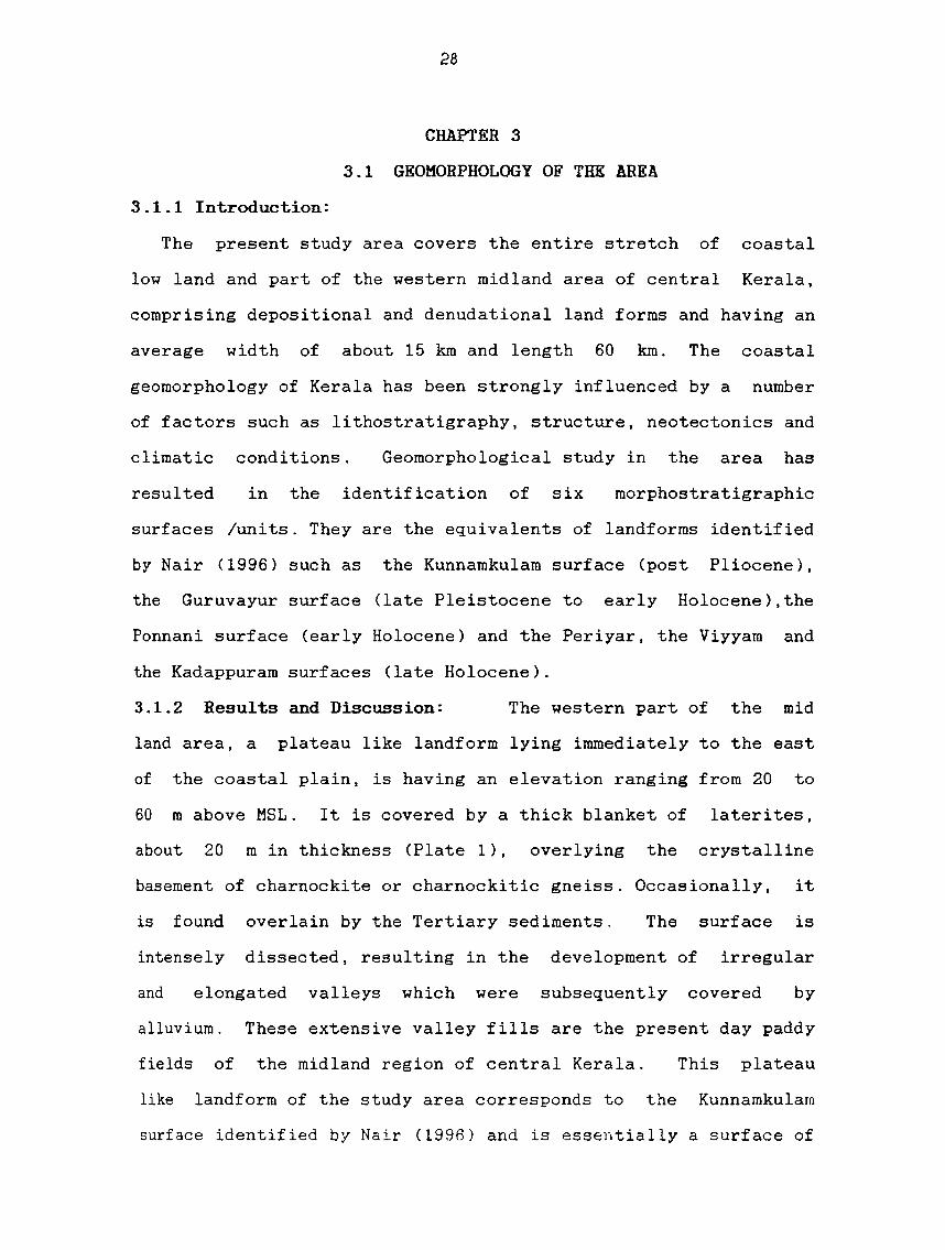
3.1.2 Results and Discussion: The western part of the mid
land area, a plateau like landform lying immediately to the east
of the coastal plain, is having an elevation ranging from 20 to
60 m above MSL. It is covered by a thick blanket of laterites,
about 20 m in thickness (Plate 1), overlying the crystalline
basement of charnockite or charnockitic gneiss. Occasionally, it
is found overlain by the Tertiary sediments. The surface is
intensely dissected, resulting in the development of irregular
and elongated valleys which were subsequently covered by
alluvium. These extensive valley fills are the present day paddy
fields of the midland region of central Kerala. This plateau
like landform of the study area corresponds to the Kunnamkulam
surface identified by Hair (1996) and is essentially a surface of
Plate 1 Primary laterlte section at l\1anJaly south east of Paravoor
Plate 2 Ridge and swale topography, Kodungallur :I rea
., ... - ..
o
,
Fig. 4. ',' Orientation of
Suchindan, 1984)
\ \ ,\
\ \
\ , .. , I , , , , , \ , \
paJaeo-beach rjdges (Source: MaJUk
:( If •
and
Plate 3 Brown coloured beach ridge sand, Kodungallur area
Plate'..J Ve~elated dune sediments. south east of P3r:l\'oor
30
directions and are essentially parallel to the present day coast.
In addition, some irregularly aligned beach ridges are seen near
the innermost palaeocoastline and are mostly composed of fine
grained white sands (Plate 4). This surface, which is currently
undergoing dissection and is tectonically active, can be of late
Pleistocene to early Holocene origin, and was named as Guruvayur
surface (Nair, 1996). In a transect about 5 km north of
Kodungallur, eight prominent palaeobeach ridges have been
identified. Further north i.e. in the Engandiyur Mullassery
transect, only six ridges have been identified whereas in
Njarakkal area only 3 prominent ridges have been found. A few
sand dunes are also noticed to the east of Pullut channel, ie. NE
of Kodungallur area. The height of the ridges varies from 2 to 6
m above MSL and the ridges exhibit a sloping pattern towards the
present coast.
According to Mathai and Nair (1988), the strand lines and
linear sand dunes of the Kodungallur area are evidences for a
periodic cyclicity in the regression of the sea, indicating
dominance of marine forces in the evolution of various land
forms. Although, they attribute that the alignment of Pullut
river and the Varapuzha river marks the earliest palaeocoastline
but in the transect north of Kodungallur, atleast two more beach
ridges have been found to the east of Pullut channel. The
orientation of these ridges as well as the colour and texture of
sediments differ much from the present day beach ridges
indicating that these eastern most ridges are the result of
earlier transgressive - regressive phases of late Pleistocene
time whereas the ridges to the west of Pullut channel are the
result of Holocene transgression and the subsequent regression.
31
The major land forms of fluvial origin are the extensive
terraces shaped mainly by Karuvannur and Periyar river systems.
All these river terraces are found at different -elevations and
have been named as the Ponnani surface (Nair, 1996). Prominent
terraces at different elevations are found at Kalamassery,
Alangad, Aduvassery - Chengamanad, Valloor, Mala, Karuvannur and
in the Koleland areas. River terraces are the result of
upgrading or down cutting of the channels due to changes in
baselevel. In this connection, they can be linked to sea level
variation. The vast remnant flood plains I river terraces range
in elevation from 1 to 5 m than the present flood plains
might have resulted from the upgradation of river channels during
the high stand of sea level around mid Holocene time.
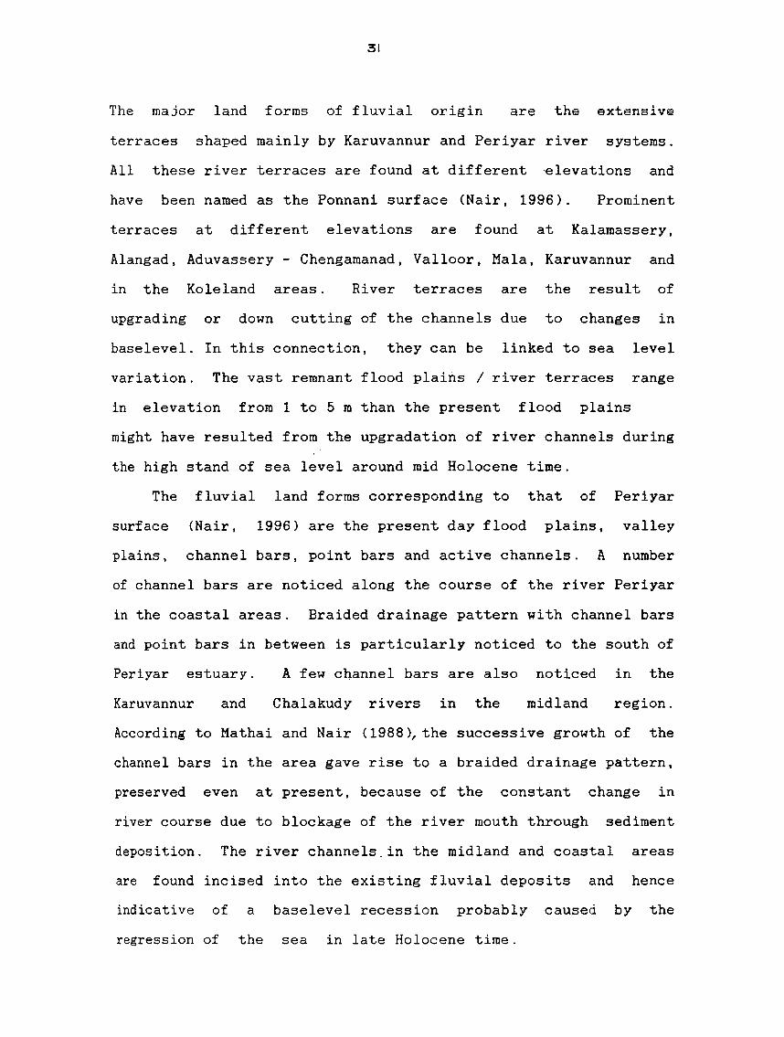
The fluvial land forms corresponding to that of Periyar
surface (Nair, 1996) are the present day flood plains, valley
plains, channel bars, point bars and active channels. A number
of channel bars are noticed along the course of the river Periyar
in the coastal areas. Braided drainage pattern with channel bars
and point bars in between is particularly noticed to the south of
Periyar estuary. A few channel bars are also noticed in the
Karuvannur and Chalakudy rivers in the midland region.
According to Mathai and Nair (1988), the successive growth of the
channel bars in the area gave rise to a braided drainage pattern,
preserved even at present, because of the constant change in
river course due to blockage of the river mouth through sediment
deposition. The river channels,in the midland and coastal areas
are found incised into the existing fluvial deposits and hence
indicative of a baselevel recession probably caused by the
regression of the sea in late Holocene time.
32
Close to the present coast line, the prominent land forms
identified
These are
equivalent
are tidal flats, mud flats, coastal
essentially fluvio-marine in origin.
of Viyyam surface of Nair's (1996)
lagoons etc.
and are the
nomenclature.
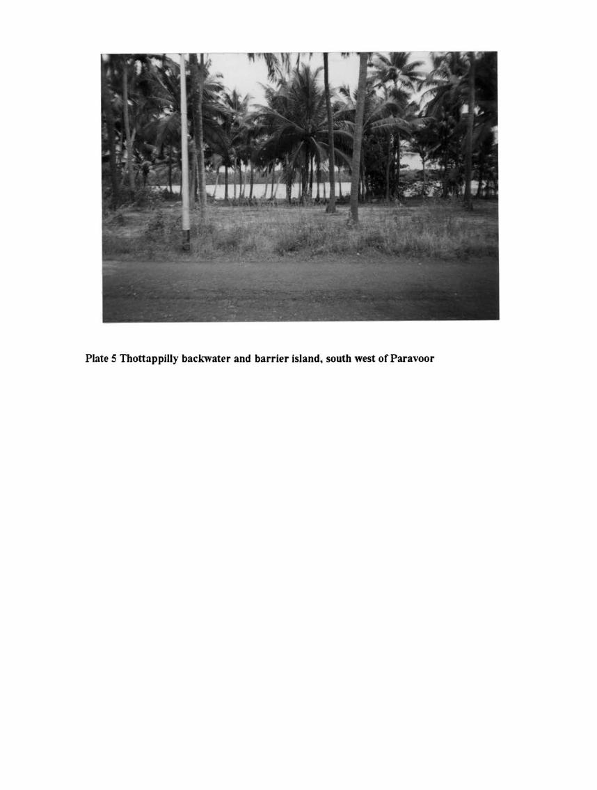
Marshy low lands are noticed at many places immediately behind
the shore lines. The lagoons occupy a considerable surface area
in central Kerala's coastal plains. The Cochin backwater system
forms part of the Vembanad lake and encompasses a number of small
islands in Ernakulam area. The northward extension of this
system is known as Thottappilly backwaters (25 km long, 1 km
wide), and runs almost parallel to the present coast separating
Vypin barrier island (Plate 5) from the main land. North of
Periyar estuary, a narrow water body known as Pullut channel (40
km long) runs parallel to the coast from Pullut to Chavakkad. At
places, it is also known as Canoli canal after a Britisher,
Canoli who was instrumental in joining this linear water body
with Periyar for transportation purpose. This channel attains
its maximum width in Kandassamkadavu area in Trichur district.
The landforms predominantly of marine origin are the present day
beaches, spits and barrier beaches. Nair (1996) has named these
landforms as Kadappuram surface. The shore line in the study
area is geometrically straight with out any cliffs. A prominent
spit is noticed at the northern end of Periyar river mouth. The
shore
coast
nature
line north of Periyar is simple whereas it is
in the southern part, showing emergent and
(Senthiappan and Rangamannar, 1978). Kunte
a compound
submergent
(1995) has
identified the Vypin - Cochin barrier island systems as the
extensive among the three barrier island systems of the
coast. On either end of the Vypin barrier island (26.5 km
most
Kerala
long
Plate 5 Thottappilly backwater and barrier island. south west of Paravoor
33
and 1 to 2.5 km wide) two narrow and elongated spits are
identified. Except the beaches at Cherai (south of Periyar) and
Koorikuzhi, others are narrow. During the southwest monsoon
season, the entire beach is subjected to severe wave erosion
resulting in the uprootment of shore line vegetation and
disturbance to human settlements.
3.1.3. Coastal Evolution
The coastal evolution along the central Kerala region is
related to the process of marine transgression and regression and
in association with coastal process such as waves, tides and
longshore currents existed during the late Quaternary period. The
presence of several sand barriers along the present day coast and
also in the recent past as exhibited by the inland barriers it is
suggested that the physical processes during mid and late
Holocene were also similar in nature. Since there are no major
delta system along this section of the coast, it is imperative
that the coast since early-mid-Iate Holocene has been subjec~to
severe physical processes where by the fluvial inputs have been
constantly reworked (Davis and Hayes, 1984).
&uriers formed during marine transgression: In a low gradient
coast whether laterally unbounded or embayed, that are subjected
to wave action at times of rising sea level are characterised by
transgressive barriers (Roy et al. , 1994) . The resulting
barriers are essentially transitory in nature that maintain
themselves in dynamic equilibrium with rising sea level by the
landward transfer of sand eroded from the shoreface, to back
barrier settings. In this study the beach ridges lying east of
Pullut channel resembles the one mentioned above. In certain
cross sections particularly east of pullut channel the barriers
are only 3 to 4rn thick and are lying right on the lateritic
surfaces. The barriers, once formed, would have shifted landward
when the sea level was rising relatively rapidly. Further when
the sea level was rising rapidly, eolian processes have also
acted simultaneously on the barriers which resulted in the
transportation of fine sands eastward over the laterite masses.
When the sea attained its maximum transgression and stable
conditions established/several small foredune complexes occurred.
Therefore from the above, it is clear that the east bank of Pullut
channel as well as beach ridges east of it and the thin veneer
of sand over the laterites have all formed
transgressive episode in the early Holocene period.
during
During
the
the
processes of landward movement of barriers either by roll over or
sand drift by wind it encloses the back swamp deposit. Thus in
this region extensive peat deposits are found below the sand
horizon.
Barriers/ridges formed during marine regression: All barriers/
sand ridges west of Pullut channel are formed by wave and wind
deposition under conditions of falling relative sea level after
6500 yrs B.P. Since all the sand ridges west of Pullut channel
slope westward it is an indication thay have formed during
regressive phase. In some southeast Australian coast, barrier
progradation was triggered through offshore influx of sand when
the sea level stabilised around 6500 yrs B.P. (Thorn et al., 1981,
Thorn and Roy, 1985). Therefore each strand plain starting from
the west bank of Pullut channel with its height ranging from 3-6m
indicate that these strand plains would have formed under a
stable sea condition followed by a fall in sea level. The sandy
materials are distributed from source area by longshore drift.
Formation of PullutlVarappuzba estuary: These represent the
remnant estuaries formed during falling sea level or stable sea
conditions through deflection of existing river courses or
formation of longshore bars which later developed into barriers.
Roy et al. (1980) have reported that the many estuaries behind
the wave built sand deposits along the southeast coast of
Australia have their origin during stable sea levels. As said
earlier in each stable condition a strand plain formed with a
swale behind which would have been a remnant estuary.
3.2. TEXTURE
3.2.1 Introduction
Sediments are the by-product of weathering. Each
environment leaves its imprint on the sediment and therefore the
various sediment characteristics can reflect their respective
environment of deposition. Grain size study is the most important
field of research in the whole spectrum of sedimentology because:
(a) the grain size is a basic descriptive measure of sedimentsi
(b) the grain size distributions may be characteristic of
sediments deposited in certain environments; (c) the grain size
distributions may yield information about the physical mechanisms
acted on the sediments during deposition and (d) the grain size
may be related to other properties such as
mineralogy,geochemistry etc. Hence, the various transportational
and depositional processes are best reflected in textural
parameters of sediments.
In the past 4-5 decades, there have been numerous attempts
to differentiate environments of deposition using grain size
parameters. Steadily the sedimentological parameters have emerged
36
as an important tool in differentiating various palaeo
environmental conditions existed through out the geological time
and also in discriminating depositional environments of recent
origin. Further, the particle size distribution of an ancient and
modern sediments have an effect on the mineralogy and chemistry
of sediments (Forstner and Wittman, 1983).
Hence, over the years, workers are able to differentiate a
number of depositional environments from size spectral analysis
as particle distribution is highly influenced by the environment
of deposition. (Folk and Ward, 1957 ; Mason and Folk, 1958;
Sahu, 1964; Friedman 1961, 1967; Hails and Hoyt, 1969; Nordstom,
1977; Goldberg 1980; Seralathan, 1979, 1986, 1988; Jahan et al.,
1990; Padmalal, 1992 and Ngusaru, 1995).
Friedman (1961, 1967) with the help of scatter diagrams of
mean versus standard deviation and sorting versus skewness of
sandy sediments
effectively used
has shown that statistical parameters
to differentiate dune, beach and
can be
river
environments. Visher (1969) has studied the log normal
distribution of grain size and was able to identify three types
of sediment populations such as rolling, saltation and
suspension; each indicative of a distinct mode of
transportational and depositional process.
Chamely et al., (1977) has used grain size pattern as one of
the parameters to study palaeoclimatic variations in the North
West African coast. Tooley (1980) has emphasized the use of
stratigraphy in palaeoenvironmental reconstruction. Yeo and Risk
(1981) have shown that the grain size analysis can be used to
study marine transgressive and regressive stratigraphy. The
Quaternary sea level history of Swartklip area in South Africa
37
has been studied by Barwis and Tankard {1983} based on sediment
facies analysis. Semeniuk and Searle (1985) have studied the
relation of past climate to different depositional facies of
calcrete sediment formation. Thorn and Roy (1985) have linked the
Holocene sea level history to patterns of sedimentation in South
East Australia. Reconstruction of palaeogeography and
palaeoenvironment of Holocene dune sediments has been carried out
by Filion {1987}. The Quaternary transgressive and regressive
episodes based on borehole sediment data in the Gulf. of Argos,
Greece have been studied by Van Andel et al. (1990). Martin and
Suguio (1992) have inferred the relative sealevel changes along
the central Brazilian coast based on palaeobeach ridge
sediments. With the help of sediment size analysis and
thermoluminescenes (TL) dating, Lees et al. (1993) have
interpreted various phases of marine transgression and dune
initiation in the early Holocene and mid Holocene periods. The
late Quaternary sealevel fluctuations in Washington area have
been inferred from the study of lake sediments by Andersen et al.
(1994).
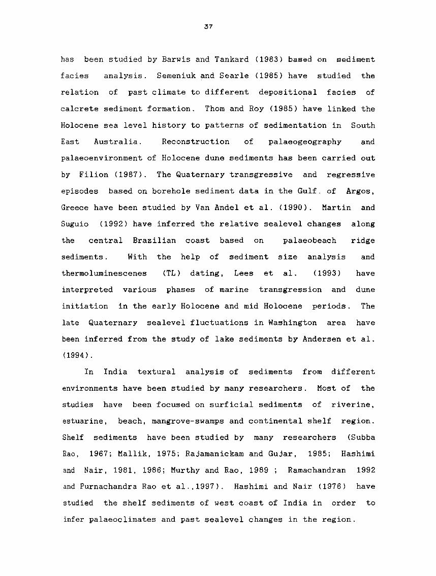
In India textural analysis of sediments from different
environments have been studied by many researchers. Most of the
studies have been focused on surficial sediments of riverine,
estuarine, beach, mangrove-swamps and continental shelf region.
Shelf sediments have been studied by many researchers (Subba
Rao, 1967; Mallik, 1975; Rajamanickam and Gujar, 1985; Hashimi
and Nair, 1981, 1986; Murthy and Rao, 1989 Ramachandran 1992
and Purnachandra Rao et al.,1997). Hashimi and Nair (1976) have
studied the shelf sediments of west coast of India in order to
infer palaeoclimates and past sealevel changes in the region.
38
By studying the shelf sediments off Gopalpur, Orissa, east
coast of India ( Rao and Rajamanickam ,198) could be able to bring
out information on low sealevel stand during Holocene.
Considerable work has been carried out on modern riverine,
estuarine and shelf sediments of the east and west coast of
India. (Kidwai, 1971; Seetaramaswamy, 1970; Satyanarayana,
1973; Veeryya and Varadachari, 1975; Seralathan 1979; Samsuddin.
1986; Chavady and Nayak 1987: Purandara et al., 1987;
Unnikrishnan, 1987; Sasidharan and Damodaran, 1988; Padmalal,
1992). Seetaramaswamy (1970) has studied the sediment texture of
the drainage system of the river Krishna on the east coast of
India. Seralathan (1979) has studied the modern deltaic
sediments of the Cauvery river and could be able to differentiate
the various depositional environments on the basis of textural
analysis. Sedimentological aspects of bottom sediments of
Vembanad lake have been carried out by Mallik and Suchindran
(1984). Padmalal (1992) has carried out a detailed granulometric
analysis of riverine and esturine sediments of central Kerala and
inferred the modern and ancient depositional regimes existed in
the area.
However, no such study has been carried out exclusively on
the Quaternary sediments on the Kerala coast. In Gujarat
coast, the Quaternary sediments have been studied by a number of
workers like Rajaguru and Marathe (1975), Gupta (1975).
Quaternary beach rocks and sediments of Maharashtra and Konkan
coast have been studied by Ghate (1985) and Wagle (1990).
Gardner (1986) has carried out detailed study of Quaternary
coastal sediments of southern Tamil Nadu coast. Hence, an attempt
has been made in this chapter to understand the particle size
39
distribution of certain selected subsurface and strand sediments
of the coastal area of central Kerala so as to have proper
insight into their origin and environments of deposition.
3.2.2. Results and Discussion
a) Strand plains sediments:
Table 1 lists the grain size parameters of 100 sediment
samples collected from the strand plains of Kodungallur area.
Table 2 gives the average values of the statistical parameters.
Mean size:- The mean size of clastic sediments is the statistical
average of grain size population expressed in phi <U>
units. Out of the 100 samples analyzed. 70 samples fall in the
medium sand range grade, 27 fine grained sand and 3 coarse
grained sand. Fig. 5 show the vertical variation of the phi mean
size from 0 to 2 m depth in all the ten sampling stations of the
Kodungallur area. At station 1, the sediments are coarser at 1
to 1.2 m level and finer at 2 m depth. Except the bottom most
sample a coarsening downward trend is observed At station 2,
finer sediments are found at the top and coarser at the bottom.
In stations 3,4,5,6,7,8 and 9 a coarsening downward trend is
observed upto a depth range 1.4 m to 1.6 m and thereafter the
sediments become finer again. A general fining downward trend is
noticed at station 10.
Standard deviation Standard deviation or sediment sorting
is the
sediment
narrow.
particle spread on either side of the
sorting is good if the spread sizes
Out of the 100 sand samples, 73 are
average. The
are relatively
moderately well
sorted, 24 moderately sorted and only 3 samples are well sorted.
In general as grain size decreases sorting improves (Fig.9). At
station 10, all ten samples are found to be only moderately
Table 1 Grain size parameters of strand sediments frol Kodungallur
Station 1 Station 4 Oepth (f\Rhi Jlean S.D Skewness Kurtosis Depth (;)Phi mean S.D Skewness Kurtosis
1.1 1.4 t.J • 0 U 11.4 U U 0 a.a 11.4 U U ... 1.4 U KY10IIe KwtoIII -., - .... 4
_Cri DIptII (Id 11 11
U ... 0.4 11.4
DJ U
0.- .. •
\I \J
\4 \4
tI tI
\J U
I I ,. 0.4 U U 1.4 • U lA !lA !lA 0 ... KInoIIa ICanDIII - ..... - .....
Depth (fA) DIptII (lit 0 11
U o.a U Cl4 OJ U 0.- .. •
\I U
\4 1.4
\J 1.1
\J U
10 U Cl4 U CU • 1.4 1.1 I. U Cl4 U U 1.1 .A KIRIM KanoIII - .... , - ....
Depth (m) DIpIft ., 0 11
D.I o.a U lA
OJ U
U CU
• 1
II \J
\4 \4
11 la U
\J I
0. ... Cl4 U D.I \J 1.4 • 11.4 ClJ eLl 1.1 1.4 •• KInoIIII 0 u ICi61DIII -_I -"'10
Fig.8 Variation of kurtosis with depth
40
sorted. Sorting does not show any clear vertical trend at
stations 1,2,3,4,5 and 8 (Fig 6). In stations 7 and 9 sorting
worsens with depth whereas it improves with depth in station 6
and 10.
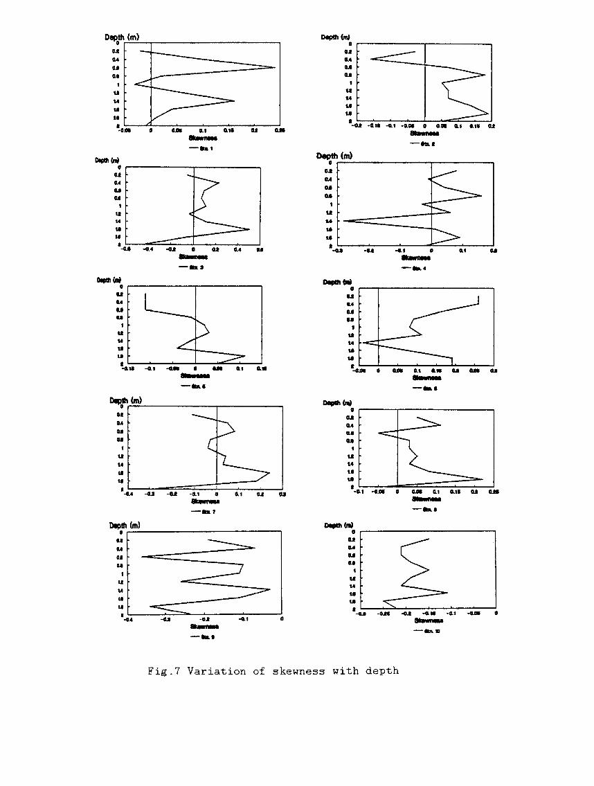
Skewness:- Skewness of the sediments is a measure of the
asymmetry of. grain size population and reflects the environment
of deposition. In textural analysis skewness is considered as an
important parameter because of its extreme sensitivity in sub
population mixing. Majority of the analysed samples show near
symmetrical skewness whereas 25 samples are coarsely skewed and
only 18 samples are finely skewed. In stations 9 and 10 coarse
skewed samples predominate. In a fine skewed sediment
population, the distribution of grains will be from coarse to
finer end and the frequency curve chops at the coarser end and
tails at the finer. Martins (1965) has suggested that the coarse
skewness in sediments could be due to two possible reasons namely
(1) addition of materials to the coarser terminal or
(2) selective removal of fine particles from a normal
population by winnowing action.
The coarse skewness may be due to selective removal of fine
population particularly in the inland region. Skewness does not
show any vertical trend with the depth in most of the stations
(Fig.7) Only in station 2 and 5 the skewness changes from
negative to positive with depth and this may be due to addition
of fine population to the existing med~~ in the prevailing
environmental condition.
Kurtosis:- Kurtosis (the peakedness of the frequency curve)
is a measure of the contrast between sorting at the central part
of the size distribution curve and that of tails. About 30 out of
41
100 samples are platykurtic, 37 meso kurtic and 33 samples are
lepto kurtic. The kurtosis does not show any vertical trend with
depth in most stations (Fig.8). In stations 1 kurtosis increases
with depth whereas it decreases in station 5 (Fig.8).
The mean size shows a decreasing trend from present
to inland except at stations 3, 4 and 8. The inner most
ridge samples are fine grained whereas sample from the
day beach and stations 4,5 and 8 are medium grained. The
tendency towards inland can be very well explained as the
beach
beach
present
fining
result
of eolian activity. The coarseness of the sediments at stations
4, 5 and 8 may be due to selective winnowing of fine sands and or
riverine input. Admixture of river sediment is very much possible
particular to station 8 as the station is situated close to the
Karuvannur
decreased
river mouth
significantly
even at present.
towards interior.
Sorting has
The inner
also
most
samples are only moderately sorted, whereas beach and near shore
samples are moderately well sorted. In general dune sediments are
very well sorted (Seralathan, 1979) whereas here only moderately
sorted sediments are observed. This deviation may be due to
admixture of very fine sand by wind deflation to the pre existing
beach ridge sediments.
While studying the depositional pattern of inter tidal
sediments in Minas basin near Novascotia, Yeo and Risk (1981)
opined that grain size distribution can be effectively used to
differentiate various Holocene depositional facies. Lees et al.,
(1993) shown that average mean size decreases from the sea coast
to flat topped, partly vegetated fore dune from 1.52 to 2.07
phi and
emplacement
again it
during
increases in beach ridge areas.
the mid Holocene is the direct result
Dune
of
42
sealevel stabilization as per the Cooper-Thorn hypothesis (Cooper,
1958). A coarsening downward trend was observed by Ngusaru (1995)
at Kunduchi and Jangwani benches of Tanzania.
Within prograded (beach ridge) barriers the basic
arrangement of facies type consisted of a burried transgressive
sand sheets underlying a regressive sequence. In many areas, the
transgressive sand sheet grades landwards into relict backbarrier
/ washover sands (Thorn and Roy, 1985). Near symmetrical skewness
is seen from the present day beach samples to interior areas
upto 6 km inland, whereas coarse skewness is seen in the inner
most stations at 9 and 10. The average values of skewness show
finely skewed only at station 6. The coarse skewness at the
interior stations can be explained as the removal of material
through eolian transportation from the already existing
palaeobeach ridge sediments. Leptokurtic samples predominate in
station closer to the present day beach whereas mesokurtic
sediments are predominant in the innermost and intermediate
stations.
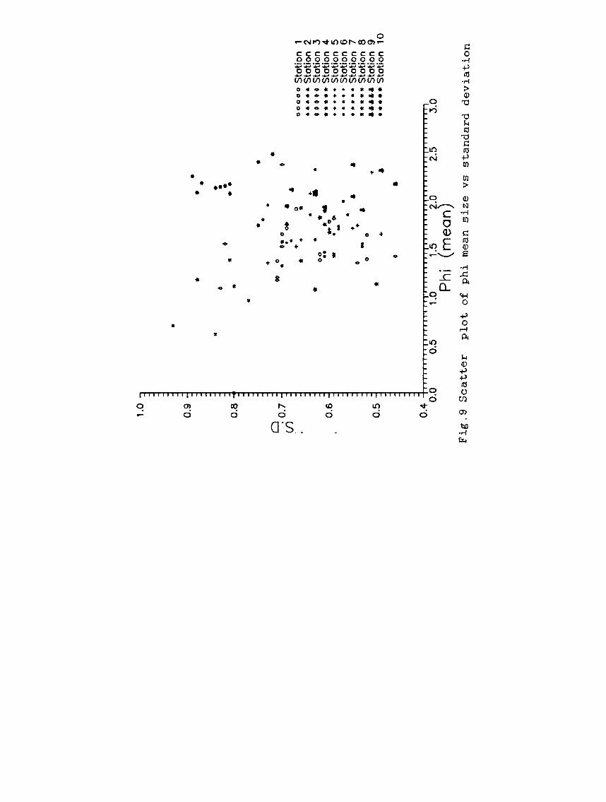
Scatter Diagrams: The scatter plot of phi mean size versus
standard deviation (Fig.9) clearly indicate that as the phi mean
size increases the sorting of the sedimnts improves. In general
the sediments of strand sediments show narrow range in phi mean
size. But the wide scattering of points ie wide variation in phi
mean size at stations 7 and 8 may be due to admixture of coarse
sand to the fine populations and so that the sediments are only
moderately sorted. Since fluvial(on a limited scale), beach,
storm and aeolian processes have acted at various levels in the
pastrthere are some variations in phi mean size from one station
to another. This is also reflected in the down core variation of
1.0
oJ ..
• *
• •
.. •
0 •
0 •
0.8
j ..
• •
.. ..
.. •
• +
•
~0.7 i
• 00
0
0 •
0.0
. ~
• "
• +
0
00
00
0 S
tatio
n
1 *
+
.. .. +
..
....
....
Sta
tion
2
* *
• *
o 0
0 0
0 S
tatio
n
.3 0
0
.. * *
* * *
' Sta
tion
4
0.6
-l
•• *'
..
*0
+
+ +
..
+ S
tatio
n
5 -
• to
-•
• •
• •
Sta
tion
6
• ..
• ..
.. t
o to
S
tatio
n
7 +
.&
.&
0
+
11
" ..
11
.. S
tatio
n
8 ...
a 0
0 ""
"aa
Sta
tion
9
0.5
-1 ..
* .&
••••• S
tatio
n
10
+
0 •
~ 0.
4 0.
0 0
.5
1.0
1.5
2.0
2.
5 P
hi
(mea
n)
Fig
.9 S
catt
er
plo
t o
f p
hi
mea
n siz
e
vs
sta
nd
ard
d
ev
iati
on
0.6
~ •
o 0
0 0
0 S
tati
on
1 0
.4 -
I ••
•••
Sta
tion
2
to 0
0 0
S
tati
on
3 **
***
Sta
tion
4
++
++
+ S
tati
on
5 •
• •
• •
• •
Sta
tion
6
• 0
• •
* ••
Sta
tion
7
tt
0 0
.2
. . ' •
tt t
t tt
•• S
tati
on
8 a
. •
.aa
aa
Sta
tion
9
en •
00
•
• +
••••• S
tati
on
10
en
* ..
..
• *
• •
ID
11
••
,& *
&
* •
o •
C
• •
• * 0
., ~
0.0
+
e
" •
• +
0
• a
• •
ID
* •
• •
• ~
• '-
.+
(f)
• &
••
-0
.2
••
a·
&
• *
a &
-0.4
~
0
-O.6~I'iTT"onMl~TTrrrn~~~~~~~~~~
0.5
1.0
1.5
2.0
2.5
Phi
(m
ean
)
Fig
.1D
S
catt
er
plo
t o
f p
hi
mea
n siz
e
vs
skew
ness
1.6
1.2
en
en
00
.8
+J
L :J
~ 0
.4
• •
* • •
• •
tit
o o
• *
0 0 0
ot+ • o
• .. •
• • ••
0 0
~ * o
o • ••
!
o "' ••
*
" ,
* *
,,"
• +
+
, •
+ ..
...
• A
· 0'·
.•
*
.: ..
A *. .
• • + • •
, o 0
00
00
S
tati
on
1 •• A
•• S
tati
on
2 to
0 •
• S
tati
on
J **
***
Sta
tion
4
• +
+ +
+ S
tati
on
5 •
• •
• •
Sta
tion
6
• ..
.. ...
. S
tati
on
7 ••
•••
Sta
tion
8
A •• A
A S
tati
on
9 , •
•••
Sta
tion
10
0.0
-tl .
, T"T
"1-r
T""
T"T
"1-r
T""
T"T
"1'"
T"r
T"T
"1'"
T"r
T"T
"1-r
T"T
"T"1
-rT
'"T
'T"'
1-r
rT'T
"'1
-rT
"rr-
1-r
T'"
T"T
'T"'
1
0.0
0.
5 1.
0 P
hi
1.5
(mea
n)
2.0
2.5
Fig
.ll
Scatt
er
plo
t o
f p
hi
mea
n siz
e
vs
ku
rto
sis
0.6
0.4
0.2
Cl)
C
l)
Q)
0.0
c 3:
Q
) ..Y
. -0
.2
if) -0
.4
-0.6
..
o
"0
o
• • * ..
• • ·0
.. •
••
,;..
.....
0
• •
....
....
...
0 +
1
»+
0"
• *
-;a •• ~+
*
& +..
...
& &
A
• &
•
& o
.. o .. ..
00
00
00
0 S
tati
on
....
....
.. S
tati
on
o 0
0 0
0 S
tati
on
****
* S
tati
on
• +
• •
+ S
tati
on
•• •
• •
Sta
tion
••••• S
tati
on
.. ...
.....
Sta
tion
&
&&
&&
Sta
tion
••
, ••
Sta
tion
• •
• .... . *
-0.8
1 i
i, i
i
i i
i i
i i
i
0.0
0.
2 0.
4 0.
6 0.
8 1
.0
S.D
1 2 3 4 5 6 7 8 9 10
Fig
.12
B
ivari
ate
p
lot
of
sta
nd
ard
d
ev
iati
on
v
s sk
ew
ness
mean size and
certain level
environment are
43
standard deviation values. That is
sediment characteristics of a
masked by the other forces and so
to say at
particular
the slight
difference in statistical variation. But in general the phi mean
size and standard deviation reflect a beach/dune environment.
The phi mean size versus skewness plot (Fig.10) shows that
majority of the sediments are near symmmetrically skewed followed
by positive and negative skewness. Only stations 9 and 10 show
negative skewness and it may be that the eolian process have
winnowed the extreme fine population. It is also evidenced from
the fact that unlike in other stations the sediments show a
narrow range of phi mean size mainly from 2 to 2.5 phi. The mean
size versus kurtosis plot (Fig.l1) indicates that as phi mean
size increases the kurtosis changes from lepto to meso and then
to platy kurtosis. However, beyond 2 phi/the kurtosis once again
becomes leptokutric due to the addition of fine population to the
existing coarse mode. The bivariant plots of standard deviation
versus skewness (Fig.12) do not show any specific trend in spite
of limited scattering of points. In general it can be said that
a good number of strand plain sediments, with well to moderately
well sorting, are symmetricl with regard to skewness. Folk and
Ward (1957) has stated that symmetrical curve may be obtained
either in a unimodal sample with good sorting or the equal
mixtures of two modes which have the poorest possible sorting for
a suite of samples. When one mode dominates the other
subordinate, the sample shows moderate sorting but gives negative
skewness as in the case of samples from stations 9 and 10.
The plots of standard deviation with kurtosis as well as
skewness and kurtosis (Figs 13 and 14) do not show any trend.
1.6
1.2
en
en
00
.8
......... L ':::J ~ 0.
4
•
A
• • 0
• *
• 4
0
.. t
• ··0
*
••
*0
•
0 :
...
°t
*,.. "
0 ..
o +
•
+
• ..
• •
CIJr .
...
+ +
.. +.
,a.
A
t ..
. -.
A
• ".
I *
A
• *
•
• 0 ••
..
• • •
, .. • o
0.0
I i
i
i i
,i
I,
i i
I '
i i
0.0
0.2
0.4
0.6
0.8
S.D
It
00
00
0 S
tati
on
A
&
A
A
&
Sta
tion
0 •••• S
tati
on
****
* S
tati
on
• +
+ +
+ S
tati
on
....
• ..
Sta
tion
..
....
. S
tati
on
.... It" S
tati
on
aa
aa
, S
tati
on
••••
• S
tati
on
1.0
Fig
.13
B
ivari
ate
p
lot
of
sta
nd
ard
d
ev
iati
on
v
s k
urt
osis
1 2 3 4 5 6 7 8 9 10
1.6
1.2
(J)
(J) 00
.8
-+-'
L
.. ::J ~ 0
.4
•
o a
* e. a e e
e e
+
* •
o • o
• *-
• o
.. o
o 0
o *
* o
a 0
0 0
• o
·
&"'
. ..
• ~
fit"
' •
• •
• e
• • . ;,
* t'"
.0
,
++
+
• • a
. a
o "' ...
"' •
~ "
'.
"'oo or
. ..
.. 0
•
o
••••• S
tatio
n
.",." S
tatio
n
11 ••• 1
1 S
tatio
n
oooo
..
oo ..
S
tatio
n
.... o
o •
Sta
tion
+
+ +
+ +
S
tatio
n
* * • *. S
tatio
n
00
00
. S
tatio
n
"'"'
"'"'
"' S
tatio
n
00
00
0 S
tatio
n
0.0
1
11
1.i
llii
lill
""
""
""
""
'I"
""
"'
••••
•• ,
I."
"il
i ••
• ,illliiil,.
-0.8
-0
.6
-0.4
-0
.2
0.0
L
'. S
kew
ne
ss
Fig
.14
B
ivari
ate
p
lot
of
skew
ness
v
s k
urt
osis
1 2 3 4 5 6 7 8 9 10
44
This may be due to the fact that most of the sediments are
normally distributed with regard to both skewness and kurtosis.
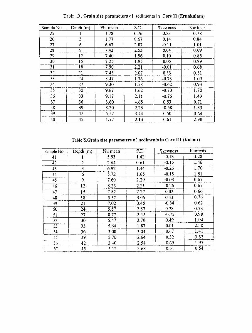
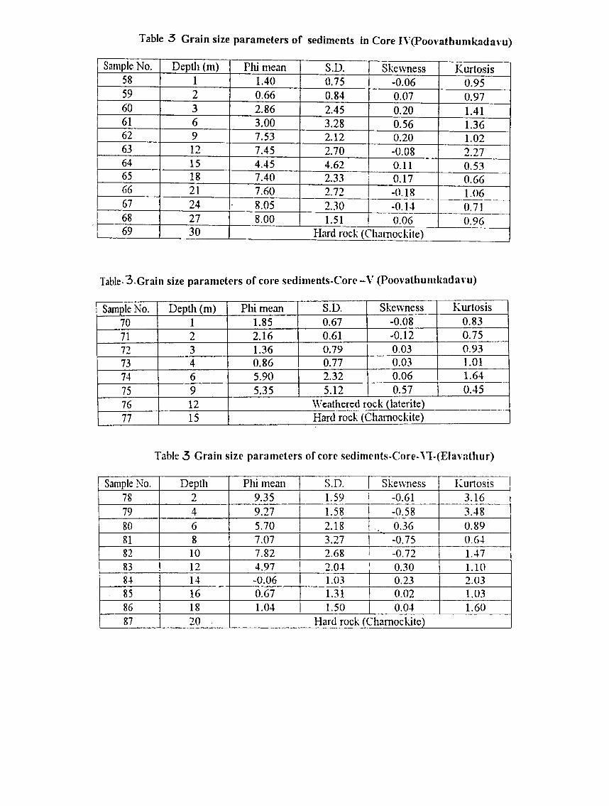
3.2.2.h. Core Sediments
Table 3 presents the grain size parameters of B7 sediment
samples collected at 1 to 3 m interval from 6 deep bore holes of
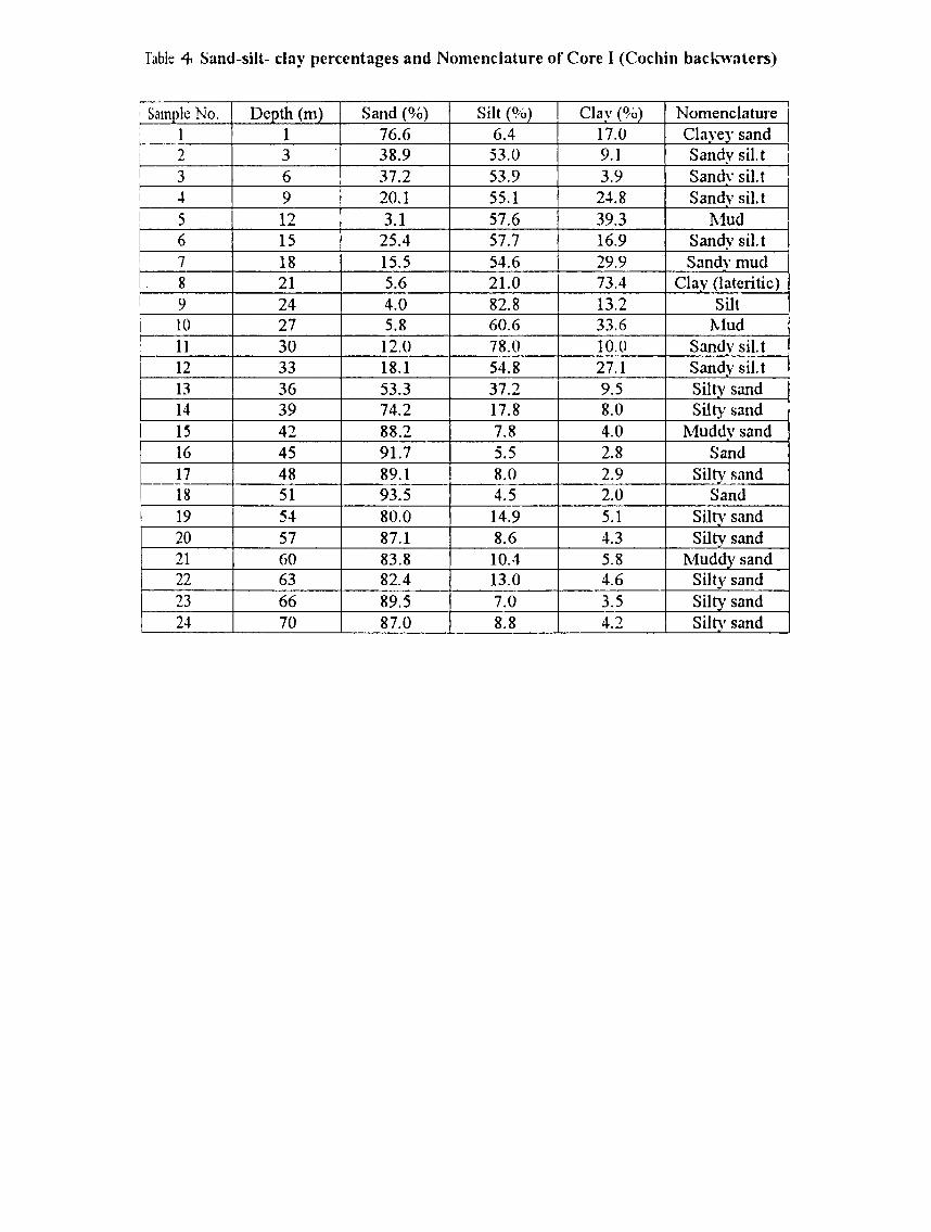
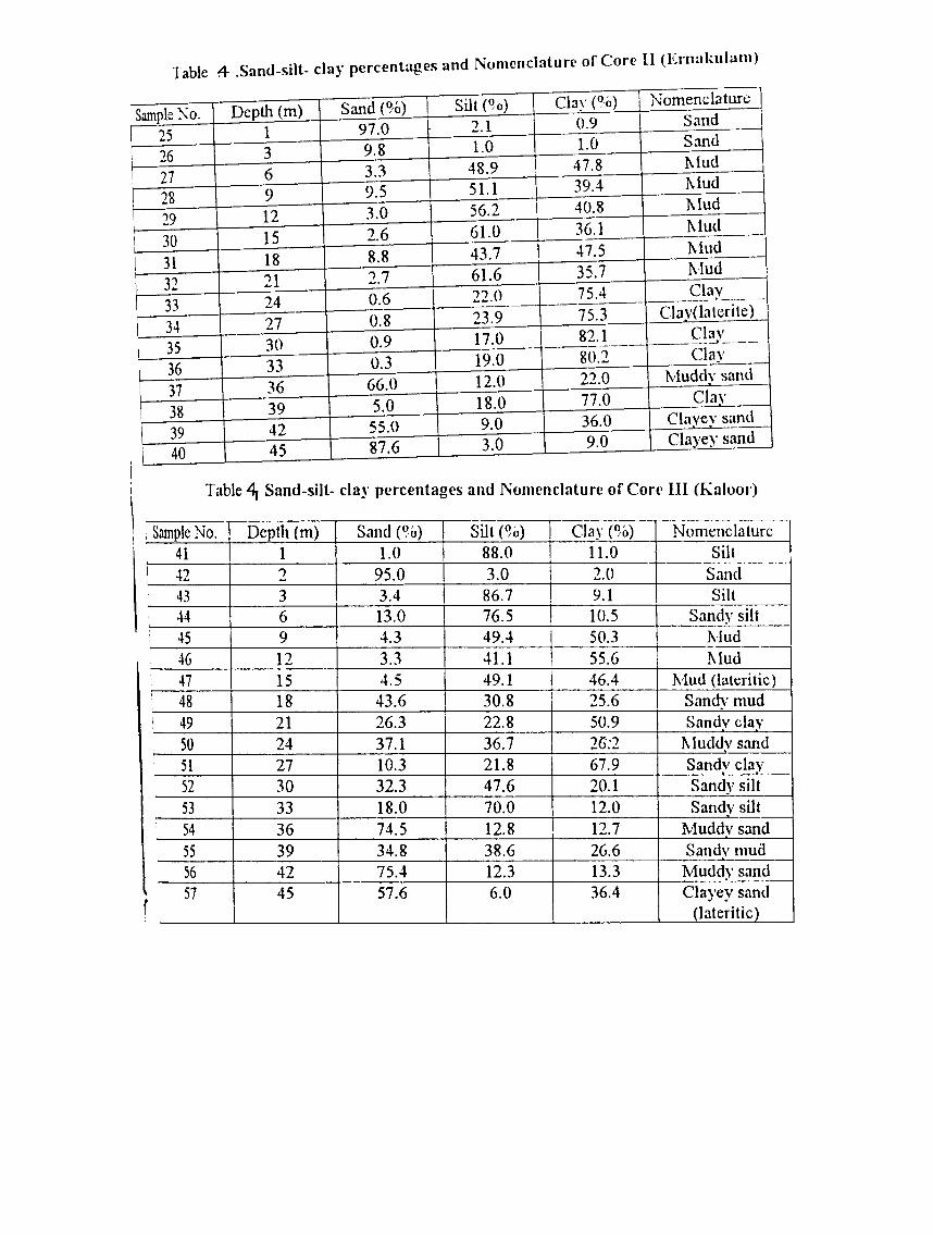
the study area. Table 4 gives the sand-silt-clay percentages and
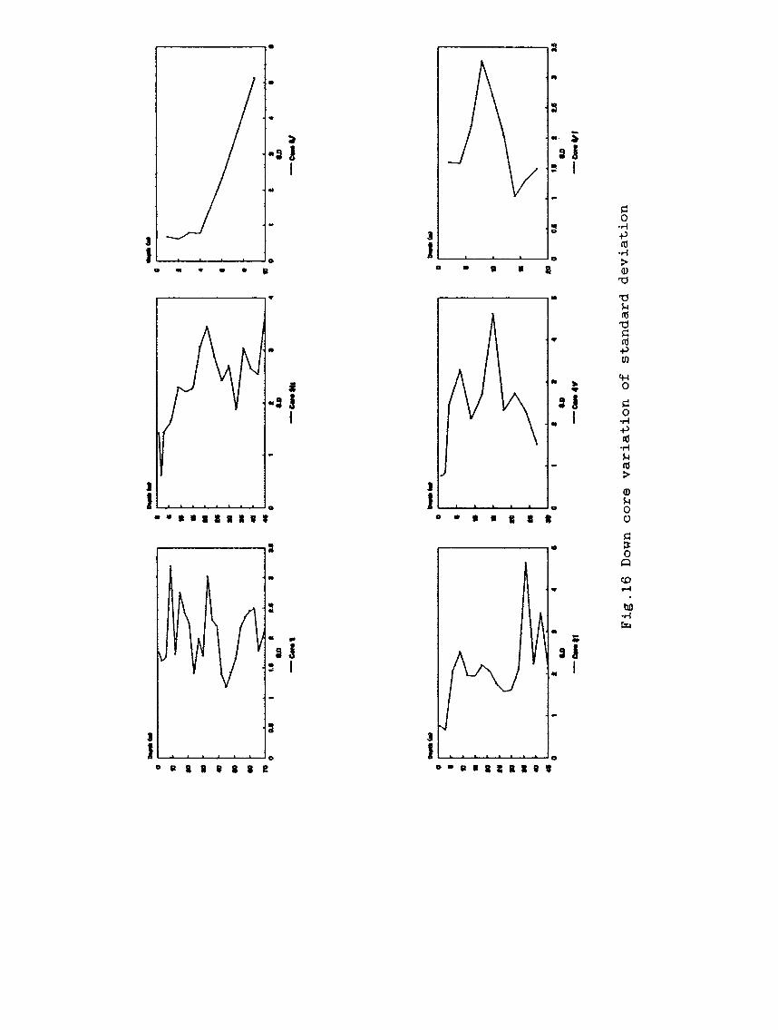
the nomenclature of the bore hole samples.The down core variation
in grain size parameters are presented in Figs.15-1B.
Mean size Fig.15 shows the variation of phi mean size with
depth in all the six cores. In core I , the phi mean size
exhibi ts a very wide range of values from 0.50 to 8.97 phi (
coarse sand to coarse clay). Coarsest sediments are found at 51
m depth and the finest at 27 m. The phi mean size is < 5 phi
upto 6 m, > 5 phi from 6 to 33 m , between 3 to 5 phi from 33 to
39 m and < 3 phi from 39 to 70 m. In core 11, the bottom most
sample (45 m) shows lower phi mean size (1.77 phi) and the
highest (9.30 phi) at 27 m depth. In this core, the phi mean
size is < 2 phi upto 3 m, 5 to 10 phi from 6 to 33 m and
again lower values at the bottom of the core. In core III
lower phi values (2.64 phi) are found at 2 m depth and higher
(8.77 phi) is seen at 27 m. From 3 to 33 m the phi mean size
ranges between 5 and 9 phi whereas lower values are found in the
bottom sediments. Weathered basement rock ie laterite lithomorge
is seen be low 45 m depth.
In core IV, samples upto 6 m show phi mean size values < 3
phi whereas from 6 m to the bottom of the core the mean size
ranges between 7 and 9 phi except at 15 m depth where it is only
4.45 phi. Hard roc k is found at 30 m depth. I n core 5, coarser
sediments « 2.1 phi) are found upto 4 m and the finer at
Table 3 . Grain size parameters of sediments in Core I (Cochin hackwaters)
Sample :';0. I Depth (m) 1 Phi mean ! SD i •• I Ske~ness Kurtosis I 1 ' 1 2.82 i 1.76 ! 0.22 1.65 \2 3 4.87 i 1.62 ! 0.53 1.21 13 6 14.92 I 1.68 10.58 ! 1.75 I 4 9 6.13 I 3.19 I -0.14 1.21 5 12 7.20 1 1.73 i -0.06 1.24
:6 15 6.02 2.75 i -0.02 0.76 7 18 6.62 I 2.42 1-0.09 1.07