76
Chapter 3 Principles of nuclear magnetic resonance and MRI Review
| Date post: | 31-Dec-2015 |
| Category: |
Documents |
| Upload: | tyrone-mooney |
| View: | 19 times |
| Download: | 1 times |

Chapter 3
Principles of nuclear magnetic resonance and MRI
Review
Basic Physics of MRI
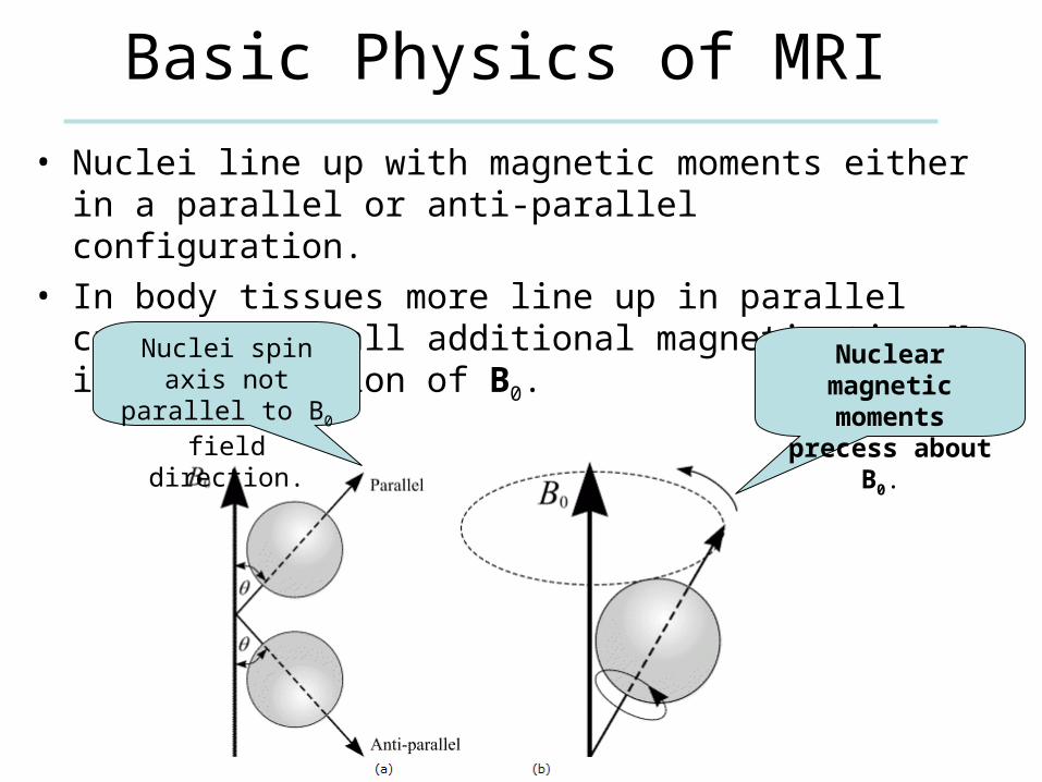
• Nuclei line up with magnetic moments either in a parallel or anti-parallel configuration.
• In body tissues more line up in parallel creating a small additional magnetization M in the direction of B0.
Nuclear magnetic moments precess
about B0.
Nuclei spin axis not parallel to B0 field
direction.
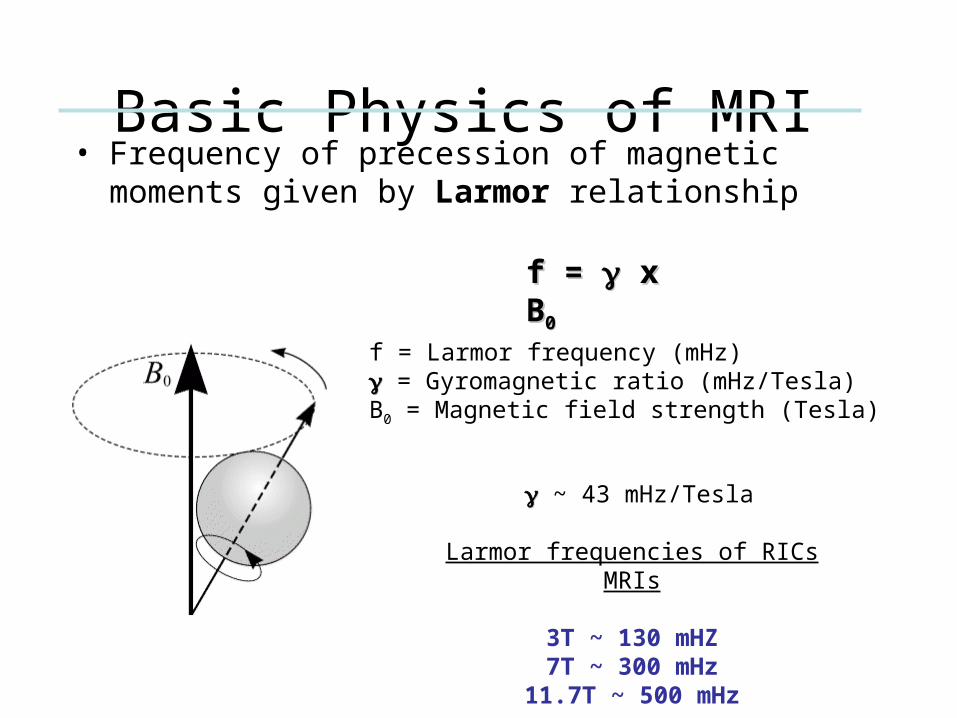
Basic Physics of MRI• Frequency of precession of magnetic moments given by
Larmor relationship
~ 43 mHz/Tesla
Larmor frequencies of RICs MRIs
3T ~ 130 mHZ7T ~ 300 mHz
11.7T ~ 500 mHz
f = f = x B x B00
f = Larmor frequency (mHz) = Gyromagnetic ratio (mHz/Tesla)B0 = Magnetic field strength (Tesla)
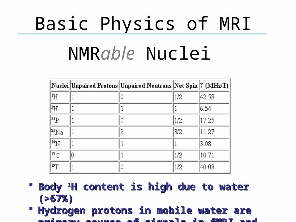
NMRable Nuclei
Basic Physics of MRI
Body Body 11H content is high due to water (>67%)H content is high due to water (>67%) Hydrogen protons in mobile water are primary Hydrogen protons in mobile water are primary
source of signals in fMRI and aMRIsource of signals in fMRI and aMRI
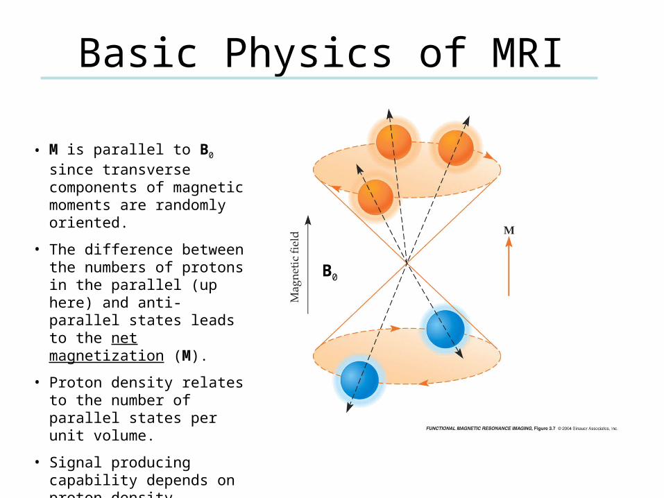
• M is parallel to B0 since transverse components of magnetic moments are randomly oriented.
• The difference between the numbers of protons in the parallel (up here) and anti-parallel states leads to the net magnetization (M).
• Proton density relates to the number of parallel states per unit volume.
• Signal producing capability depends on proton density.
Basic Physics of MRI
B0
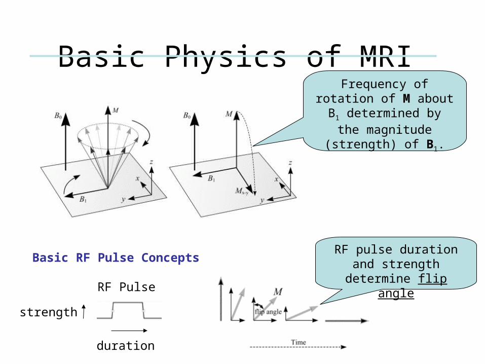
Basic Physics of MRI
RF pulse duration and strength determine flip
angle
duration
strength
RF Pulse
Frequency of rotation of M about B1 determined by the magnitude (strength)
of B1.
Basic RF Pulse Concepts

Basic Physics of MRI
FID magnitude decays in an exponential manner with a time constant T2. Decay due to spin-spin relaxation.
• 90° RF pulse rotates M into transverse (x-y) plane
• Rotation of M within transverse plane induces signal in receiver coil at Larmor frequency.
• Magnitude signal dependent on proton density and Mxy. )2sin()( 2
0 fteStS Tt
π⋅=−
FID = Free Induction Decay
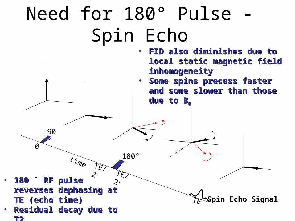
Need for 180° Pulse - Spin Echo
90°
180°0
TE
TE/2 -
timeTE/2+
• FID also diminishes due to local static FID also diminishes due to local static magnetic field inhomogeneitymagnetic field inhomogeneity
• Some spins precess faster and some Some spins precess faster and some slower than those due to Bslower than those due to B00
• 180 180 ° RF pulse reverses RF pulse reverses dephasing at TE (echo time)dephasing at TE (echo time)
• Residual decay due to T2Residual decay due to T2 Spin Echo Signal
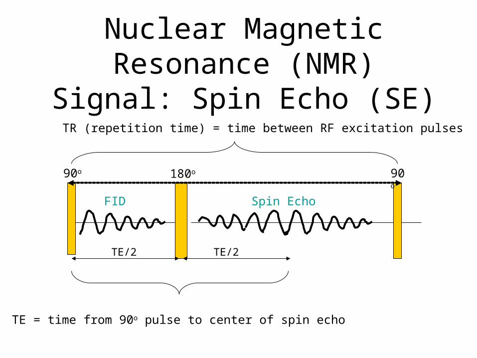
Nuclear Magnetic Resonance (NMR) Signal: Spin Echo (SE)
TE/2 TE/2
90o
TR (repetition time) = time between RF excitation pulses
90o 180o
FID Spin Echo
TE = time from 90o pulse to center of spin echo
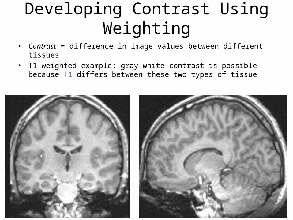
Developing Contrast Using Weighting
• Contrast = difference in image values between different tissues
• T1 weighted example: gray-white contrast is possible because T1 differs between these two types of tissue
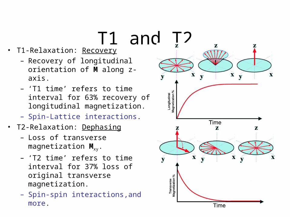
T1 and T2• T1-Relaxation: Recovery
– Recovery of longitudinal orientation of M along z-axis.
– ‘T1 time’ refers to time interval for 63% recovery of longitudinal magnetization.
– Spin-Lattice interactions.
• T2-Relaxation: Dephasing
– Loss of transverse magnetization Mxy.
– ‘T2 time’ refers to time interval for 37% loss of original transverse magnetization.
– Spin-spin interactions,and more.
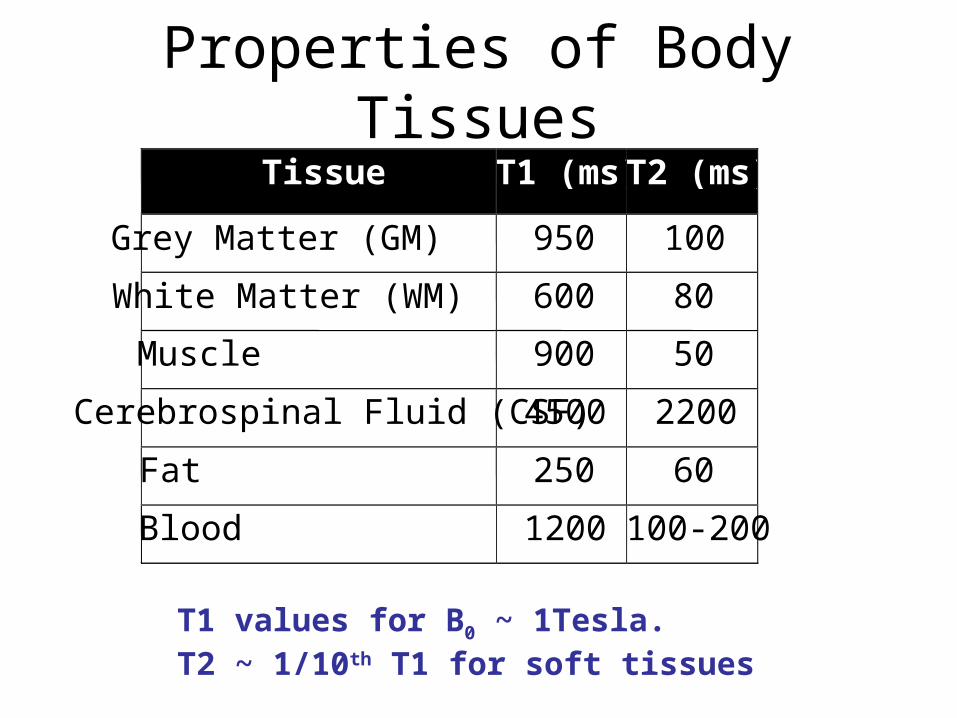
Properties of Body Tissues
Tissue T1 (ms) T2 (ms)
Grey Matter (GM) 950 100
White Matter (WM) 600 80
Muscle 900 50
Cerebrospinal Fluid (CSF) 4500 2200
Fat 250 60
Blood 1200 100-200
T1 values for B0 ~ 1Tesla.T2 ~ 1/10th T1 for soft tissues

Basic Physics of MRI: T1 and T2
T1 is shorter in fat (large molecules) and longer in
CSF (small molecules). T1 contrast is higher for lower
TRs.
T2 is shorter in fat and longer in CSF. Signal
contrast increased with TE.
• TR determines T1 contrast
• TE determines T2 contrast.
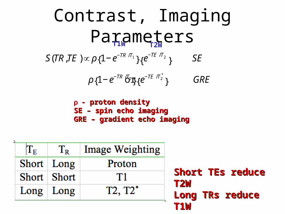
Contrast, Imaging Parameters
- proton density- proton densitySE – spin echo imagingSE – spin echo imagingGRE – gradient echo imagingGRE – gradient echo imaging
Short TEs reduce T2WShort TEs reduce T2WLong TRs reduce T1WLong TRs reduce T1W
€
S(TR,TE)∝ ρ 1− e−TR /T1{ } e−TE /T2{ } SE
or ρ 1− e−TR /T1{ } e−TE /T2*
{ } GRE
T1W T2W
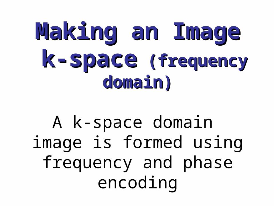
Making an ImageMaking an Image k-space k-space (frequency domain) (frequency domain)
A k-space domain image is formed using frequency
and phase encoding
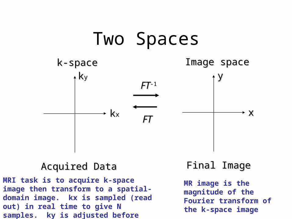
Two Spaces
FTFT
FTFT-1-1
k-spacek-space
kkxx
kkyy
Acquired DataAcquired Data
Image spaceImage space
xx
yy
Final ImageFinal Image
MRI task is to acquire k-space image then transform to a spatial-domain image. kx is sampled (read out) in real time to give N samples. ky is adjusted before each readout.
MR image is the magnitude of the Fourier transform of the k-space image
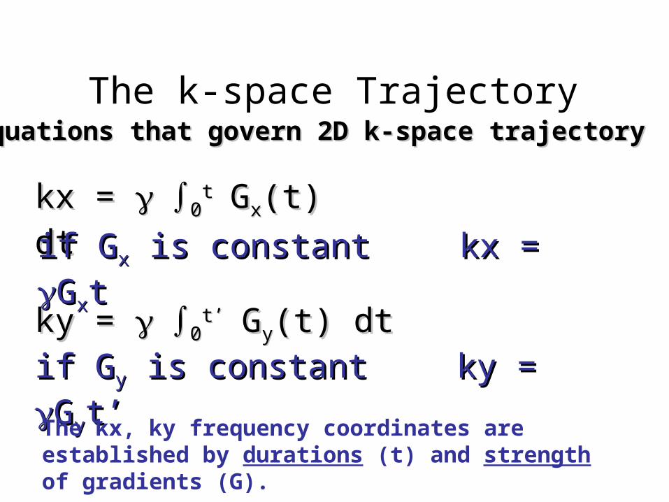
The k-space Trajectory
kx = kx = 00ttGGxx(t) dt(t) dt
ky = ky = 00t’t’GGyy(t) dt(t) dt
if Gif Gyy is constant is constant ky = ky = GGyyt’t’
Equations that govern 2D k-space trajectoryEquations that govern 2D k-space trajectory
The kx, ky frequency coordinates are established by durations (t) and strength of gradients (G).
if Gif Gxx is constant is constant kx = kx = GGxxtt

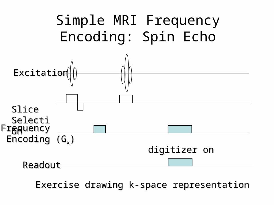
Simple MRI Frequency Encoding:
digitizer ondigitizer on
RF ExcitationRF Excitation
SliceSliceSelection (GSelection (Gzz))
FrequencyFrequency Encoding (GEncoding (Gxx))
ReadoutReadout
Exercise drawing k-space manipulationExercise drawing k-space manipulation
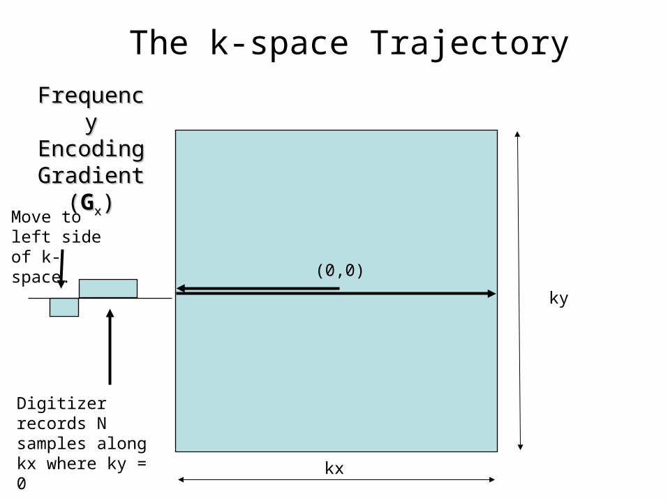
The k-space Trajectory
Frequency Frequency Encoding Encoding Gradient Gradient
((GGxx))
kx
ky
(0,0)
Digitizer records N samples along kx where ky = 0
Move to left side of k-space.
Simple MRI Frequency Encoding: Spin Echo
digitizer ondigitizer on
ExcitationExcitation
SliceSliceSelectionSelection
FrequencyFrequency Encoding (GEncoding (Gxx))
ReadoutReadout
Exercise drawing k-space representationExercise drawing k-space representation

The K-space Trajectory
180 pulse
Digitizer records N samples of kx where ky = 0
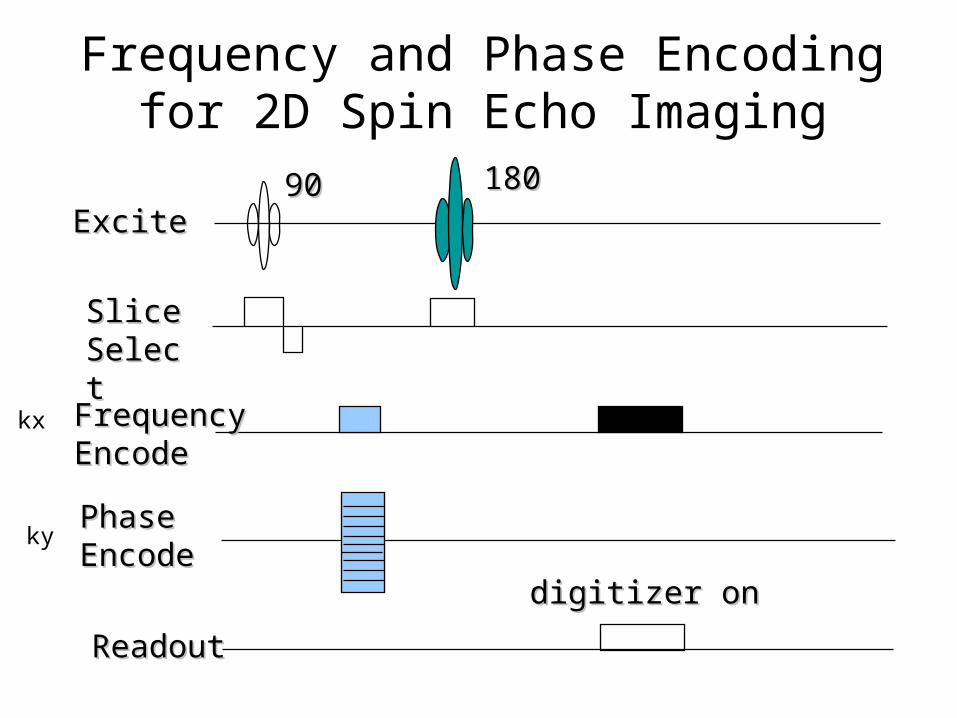
Frequency and Phase Encoding for 2D Spin Echo Imaging
digitizer ondigitizer on
ExciteExcite
SliceSliceSelectSelect
FrequencyFrequencyEncodeEncode
PhasePhaseEncodeEncode
ReadoutReadout
9090 180180
kx
ky
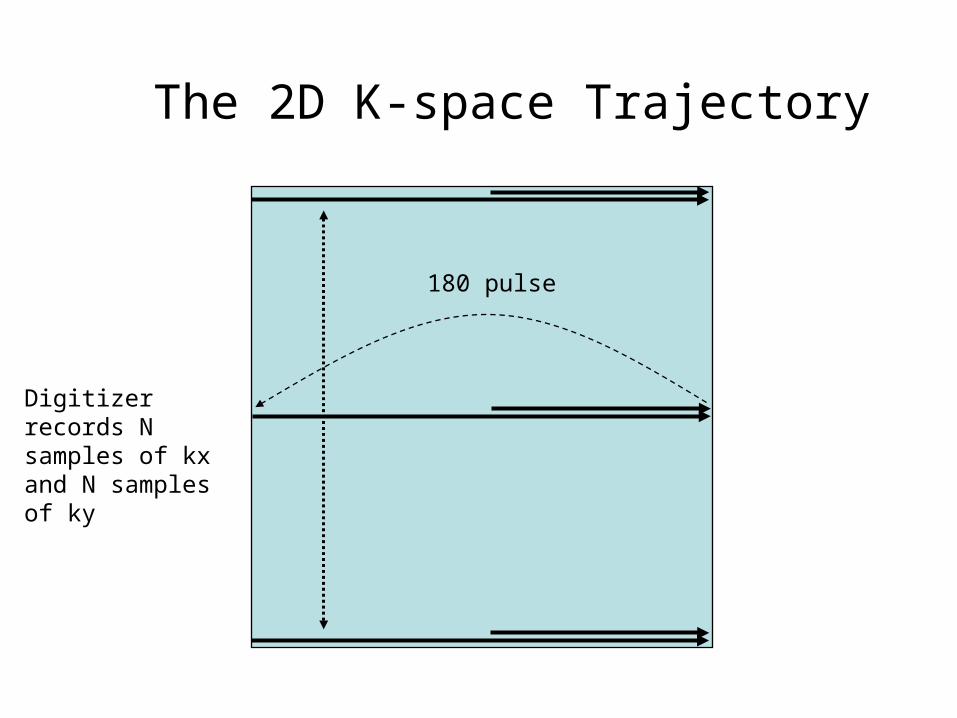
The 2D K-space Trajectory
180 pulse
Digitizer records N samples of kx and N samples of ky
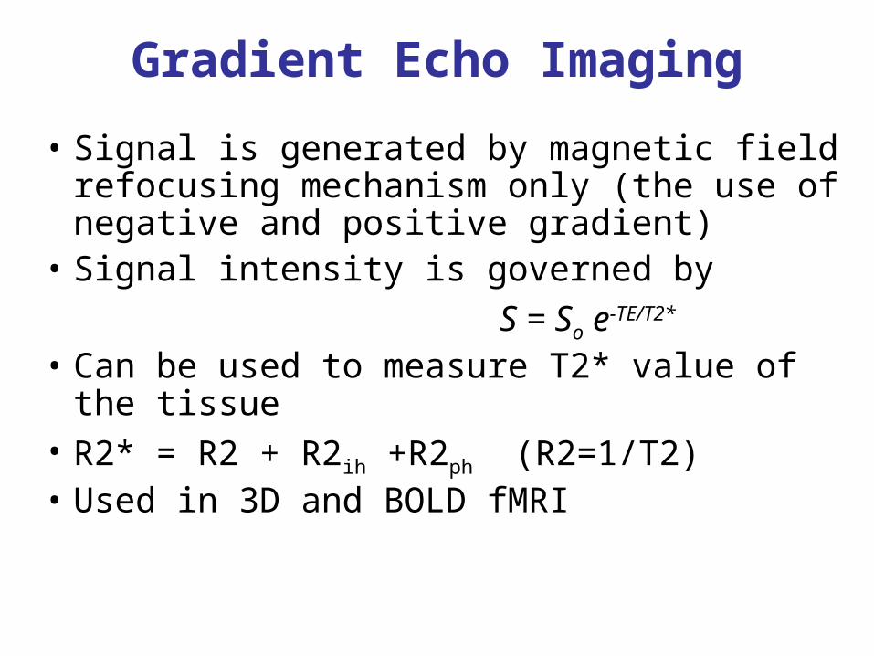
Gradient Echo Imaging
• Signal is generated by magnetic field refocusing mechanism only (the use of negative and positive gradient)
• Signal intensity is governed by
S = So e-TE/T2*
• Can be used to measure T2* value of the tissue• R2* = R2 + R2ih +R2ph (R2=1/T2)• Used in 3D and BOLD fMRI
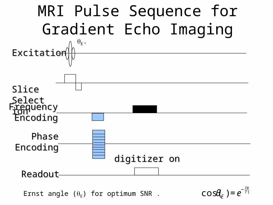
MRI Pulse Sequence for Gradient Echo Imaging
digitizer ondigitizer on
ExcitationExcitation
SliceSliceSelectionSelection
FrequencyFrequency EncodingEncoding
PhasePhase EncodingEncoding
ReadoutReadout
€
cos(θE ) = e− TRT1Ernst angle (E) for optimum SNR .
E.
crus
her
crus
her
crus
her
crus
her
B1
Gz
Gx
Gy
B1
Gz
Gx
Gy
TR1 TR2
TRN/2 TRN
TR1
TR2
TRN/2
TRN
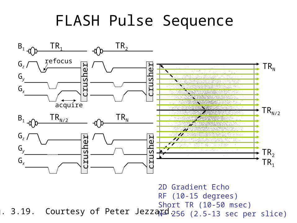
Fig. 3.19. Courtesy of Peter Jezzard.
refocus
acquire
FLASH Pulse Sequence
2D Gradient EchoRF (10-15 degrees)Short TR (10-50 msec)N= 256 (2.5-13 sec per slice)
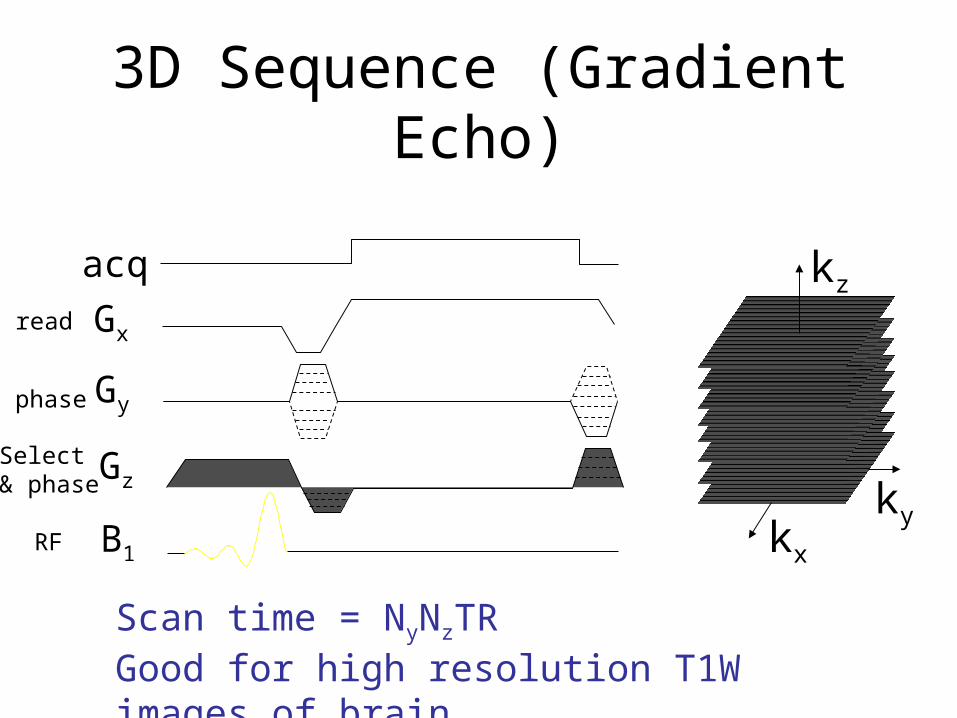
3D Sequence (Gradient Echo)
Gx
Gy
Gz
B1
acq
kx
ky
kz
Scan time = NyNzTRGood for high resolution T1W images of brain
Select& phase
phase
read
RF
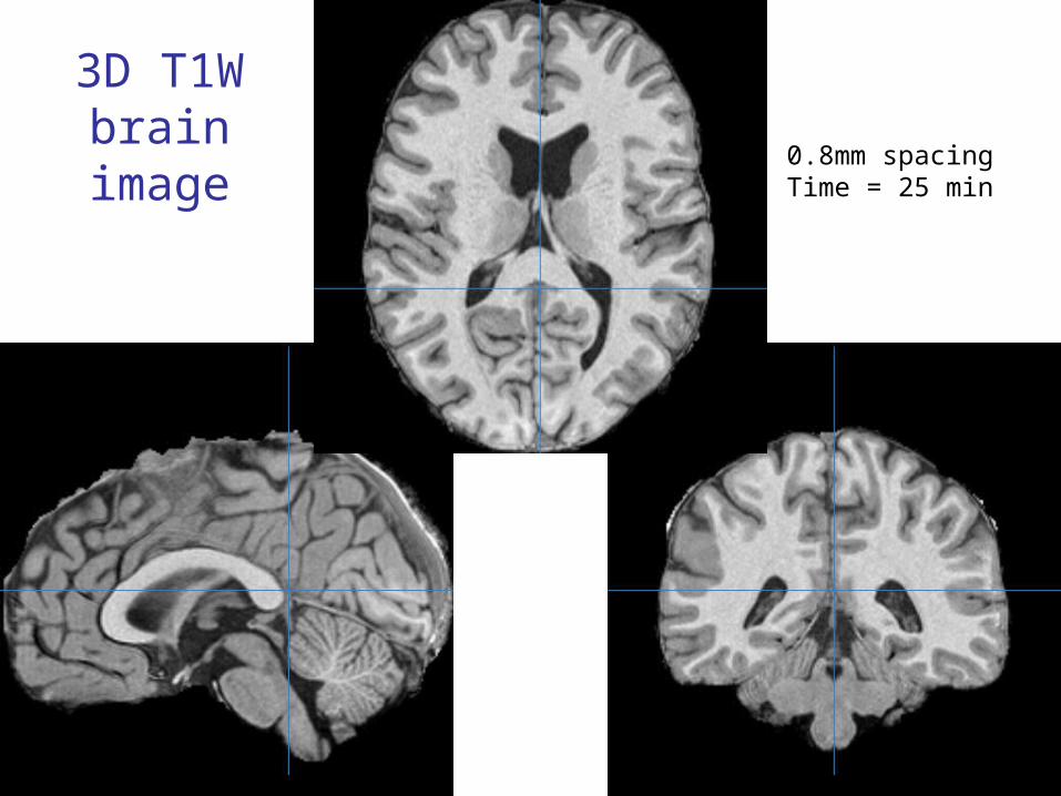
3D T1W brain image 0.8mm spacing
Time = 25 min
B1
Gz
Gx
Gy
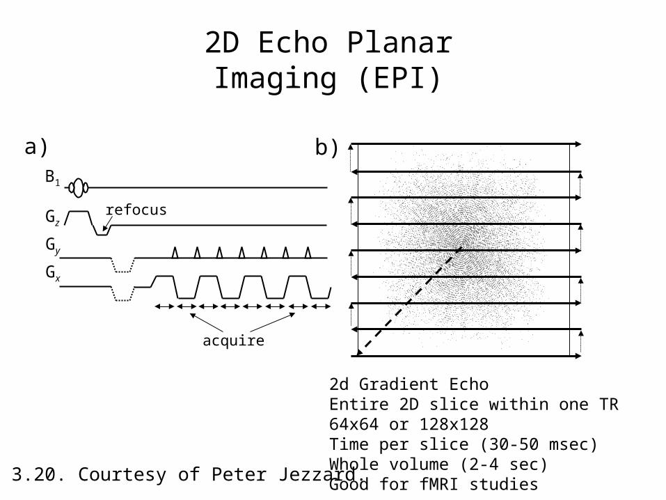
Fig. 3.20. Courtesy of Peter Jezzard.
refocus
acquire
a) b)
2D Echo Planar Imaging (EPI)
2d Gradient EchoEntire 2D slice within one TR64x64 or 128x128Time per slice (30-50 msec)Whole volume (2-4 sec)Good for fMRI studies
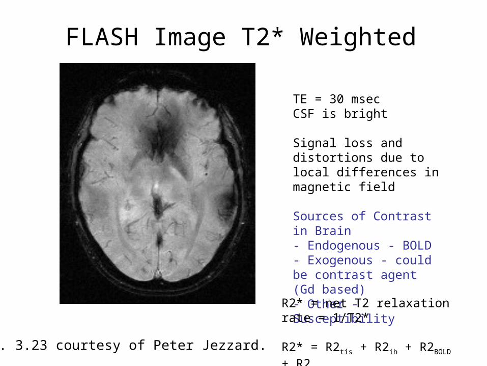
Fig. 3.23 courtesy of Peter Jezzard.
FLASH Image T2* Weighted
TE = 30 msecCSF is bright
Signal loss and distortions due to local differences in magnetic field
Sources of Contrast in Brain- Endogenous - BOLD- Exogenous - could be contrast agent (Gd based)- Other - Susceptibility
R2* = net T2 relaxation rate = 1/T2*
R2* = R2tis + R2ih + R2BOLD + R2suc
Chapter 8
Quantitative Measurements Using fMRI
Review
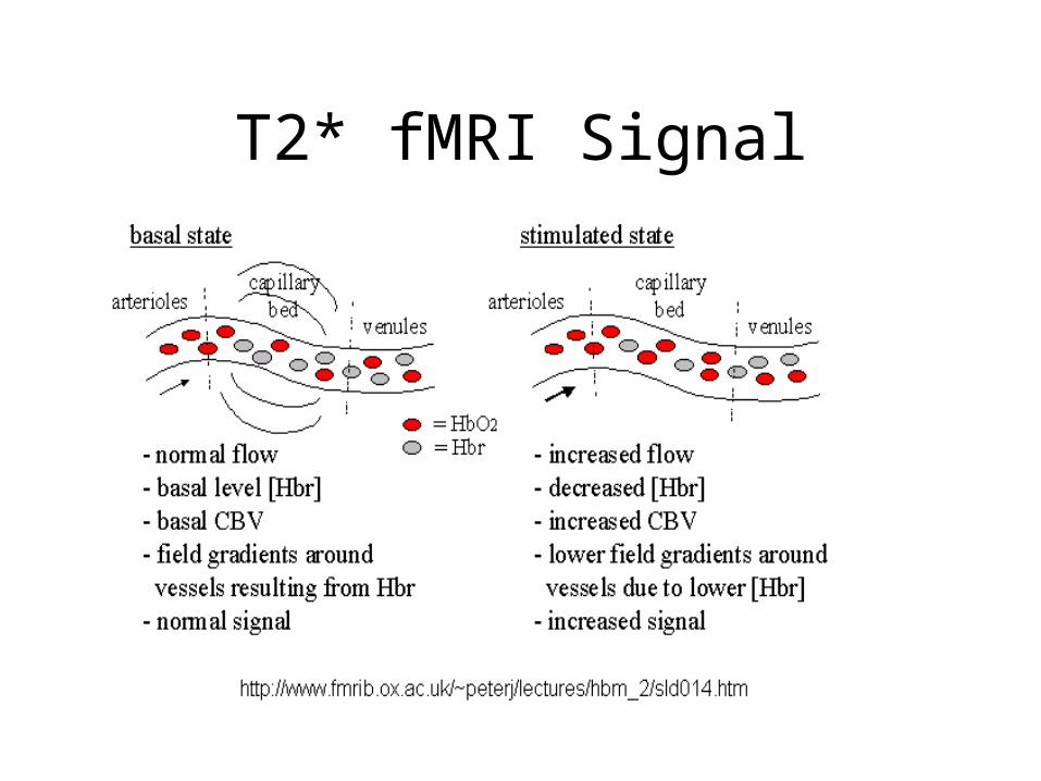
T2* fMRI Signal
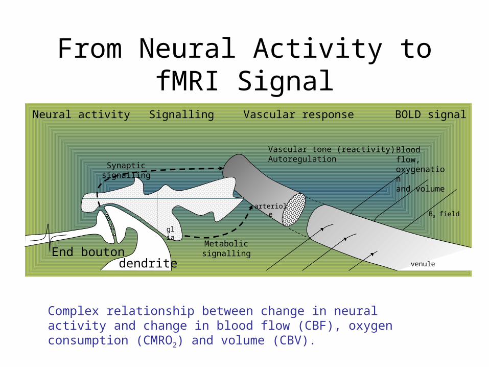
From Neural Activity to fMRI Signal
Neural activity Signalling Vascular response
Vascular tone (reactivity)Autoregulation
Metabolic signalling
BOLD signal
glia
arteriole
venule
B0 field
Synaptic signalling
Blood flow,oxygenationand volume
Complex relationship between change in neural activity and change in blood flow (CBF), oxygen consumption (CMRO2) and volume (CBV).
dendriteEnd bouton
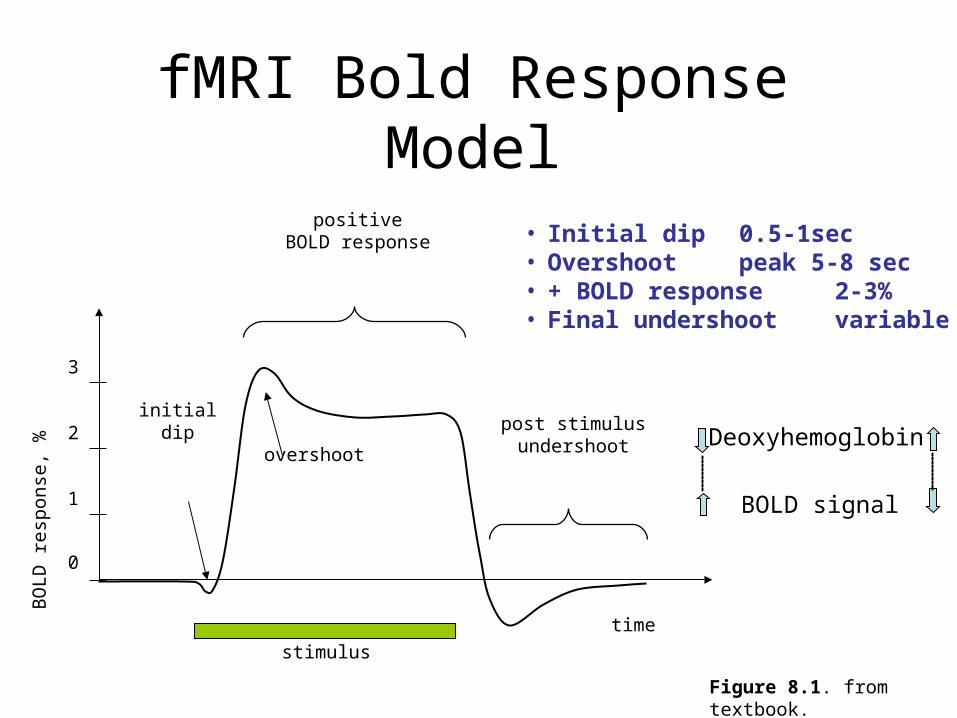
fMRI Bold Response Model
time
BO
LD
res
pons
e, %
initialdip
positiveBOLD response
post stimulusundershootovershoot
1
2
3
0
stimulus
Figure 8.1. from textbook.
• Initial dip 0.5-1sec• Overshoot peak 5-8 sec• + BOLD response 2-3%• Final undershoot variable
Deoxyhemoglobin
BOLD signal
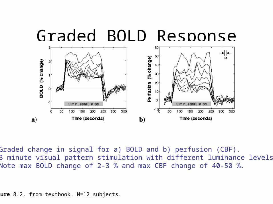
Graded BOLD Response
Figure 8.2. from textbook. N=12 subjects.
• Graded change in signal for a) BOLD and b) perfusion (CBF).• 3 minute visual pattern stimulation with different luminance levels.• Note max BOLD change of 2-3 % and max CBF change of 40-50 %.
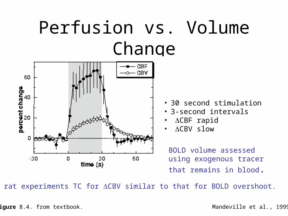
Perfusion vs. Volume Change
Figure 8.4. from textbook.
• 30 second stimulation• 3-second intervals• CBF rapid• CBV slow
Mandeville et al., 1999
In rat experiments TC for CBV similar to that for BOLD overshoot.
BOLD volume assessed using exogenous tracer that remains in
blood.
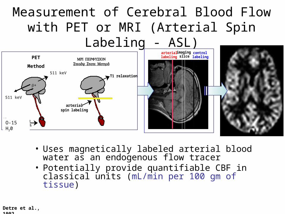
Measurement of Cerebral Blood Flowwith PET or MRI (Arterial Spin Labeling - ASL)
• Uses magnetically labeled arterial blood water as an endogenous flow tracer
• Potentially provide quantifiable CBF in classical units (mL/min per 100 gm of tissue)
Detre et al., 1992
arteriallabeling
controllabeling
imagingslice
T1 relaxation
arterialspin labeling
O infusionor inhalation
15
αdecay
PET or SPECT Steady State Method
MRI PERFUSION Steady State Method
+
511 keV
511 keV
PET
Method
O-15 H20
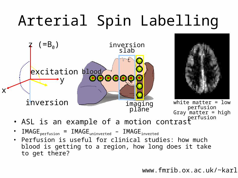
Arterial Spin Labelling
• ASL is an example of a motion contrast• IMAGEperfusion = IMAGEuninverted – IMAGEinverted
• Perfusion is useful for clinical studies: how much blood is getting to a region, how long does it take to get there?
www.fmrib.ox.ac.uk/~karla/
inversionslab
imagingplane
excitation
inversion
xy
z (=B0)
bloodblood
white matter = low perfusion
Gray matter = high perfusion
Chapter 5
Hardware for MRI
Review
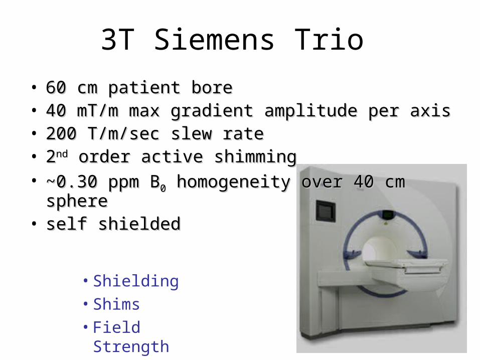
3T Siemens Trio
• 60 cm patient bore60 cm patient bore• 40 mT/m max gradient amplitude per axis40 mT/m max gradient amplitude per axis• 200 T/m/sec slew rate200 T/m/sec slew rate• 22ndnd order active shimming order active shimming• ~0.30 ppm B~0.30 ppm B00 homogeneity over 40 cm sphere homogeneity over 40 cm sphere• self shieldedself shielded
• Shielding
• Shims
• Field Strength
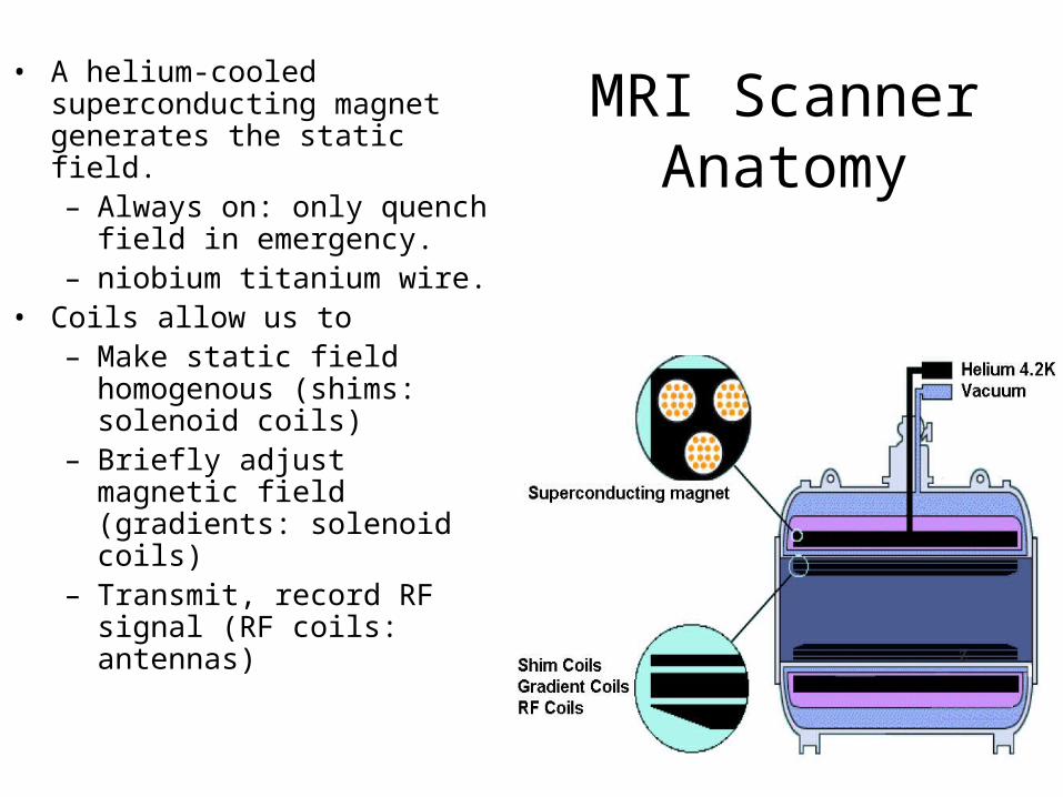
MRI Scanner Anatomy
• A helium-cooled superconducting magnet generates the static field.– Always on: only quench field in
emergency.– niobium titanium wire.
• Coils allow us to – Make static field homogenous
(shims: solenoid coils)– Briefly adjust magnetic field
(gradients: solenoid coils)– Transmit, record RF signal (RF
coils: antennas)
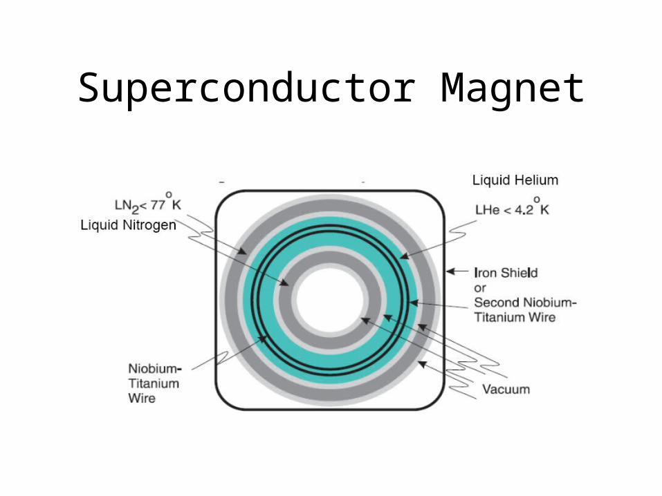
Superconductor Magnet
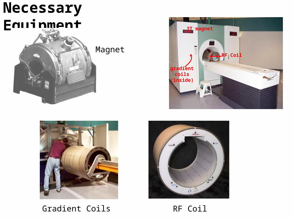
Necessary Equipment
Magnet
Gradient Coils RF Coil
RF Coil
3T magnet
gradient coils(inside)
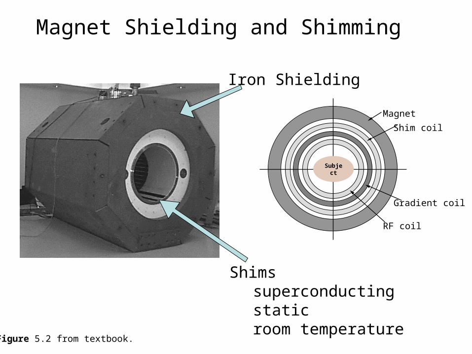
Figure 5.2 from textbook.
Magnet Shielding and Shimming
Iron Shielding
Shimssuperconductingstaticroom temperature
Magnet
Shim coil
Gradient coil
RF coil
Subject
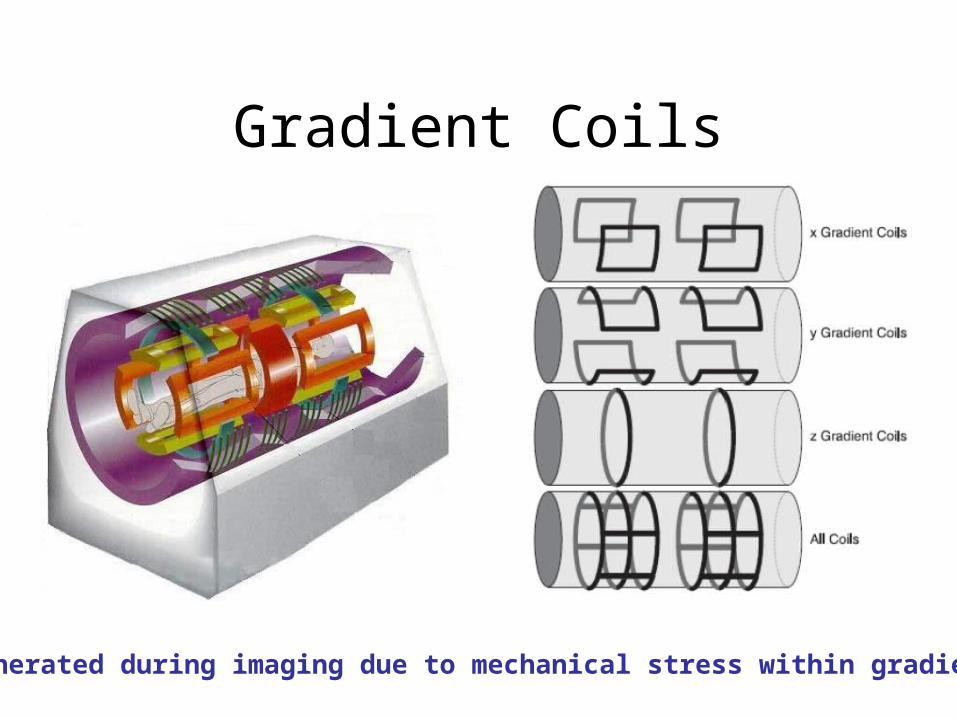
Gradient Coils
Sounds generated during imaging due to mechanical stress within gradient coils.
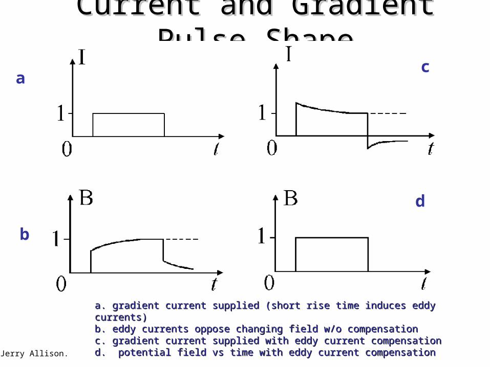
Current and Gradient Pulse ShapeCurrent and Gradient Pulse Shape
a. gradient current supplied (short rise time induces eddy currents)a. gradient current supplied (short rise time induces eddy currents) b. eddy currents oppose changing field w/o compensationb. eddy currents oppose changing field w/o compensation c. gradient current supplied with eddy current compensationc. gradient current supplied with eddy current compensation d. potential field vs time with eddy current compensationd. potential field vs time with eddy current compensation
a
d
c
b
Jerry Allison.
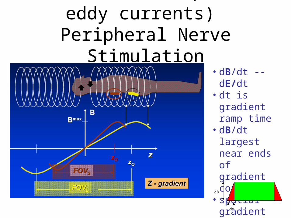
dB/dt Effect (more eddy currents)
Peripheral Nerve Stimulation• dB/dt -- dE/dt• dt is gradient
ramp time• dB/dt largest
near ends of gradient coils
• spatial gradient of dE/dt also important
dB
dt
dB/dt / E-Field Characteristics of Stimulation
• Not dependent on B0
• Gradients - 40mT/m (larger Bmax for longer coil)• Gradient Coil Differences - strength (increases dB)
and length (head vs. body determines site)• Rise Time - shorter rise time means larger shorter dt
and therefore larger dB/dt• Other
– Disruption of nearby medical electronic devices– Subject Instructions
• Don’t clasp hands - closed circuit, lower threshold• Report tingling, muscle twitching, painful sensations
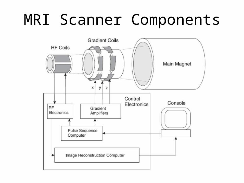
MRI Scanner Components
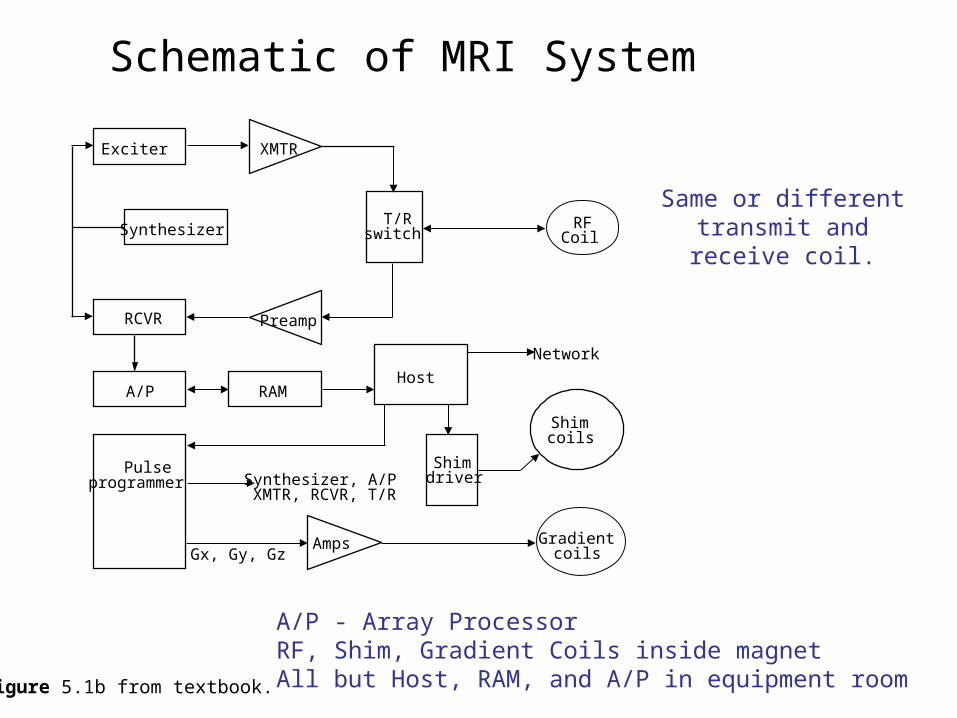
Figure 5.1b from textbook.
Exciter
Synthesizer
XMTR
T/Rswitch
RFCoil
PreampRCVR
A/P RAMHost
Pulseprogrammer Synthesizer, A/P
XMTR, RCVR, T/R
Shimdriver
Shim coils
Gradient coils
AmpsGx, Gy, Gz
Network
Schematic of MRI System
A/P - Array ProcessorRF, Shim, Gradient Coils inside magnetAll but Host, RAM, and A/P in equipment room
Same or different transmit and receive coil.
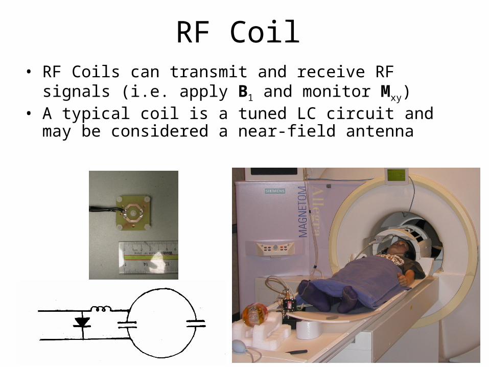
RF Coil• RF Coils can transmit and receive RF signals (i.e. apply B1
and monitor Mxy)• A typical coil is a tuned LC circuit and may be considered a
near-field antenna
NS
M-P
035
Per
man
ent
Mag
net
MR
I
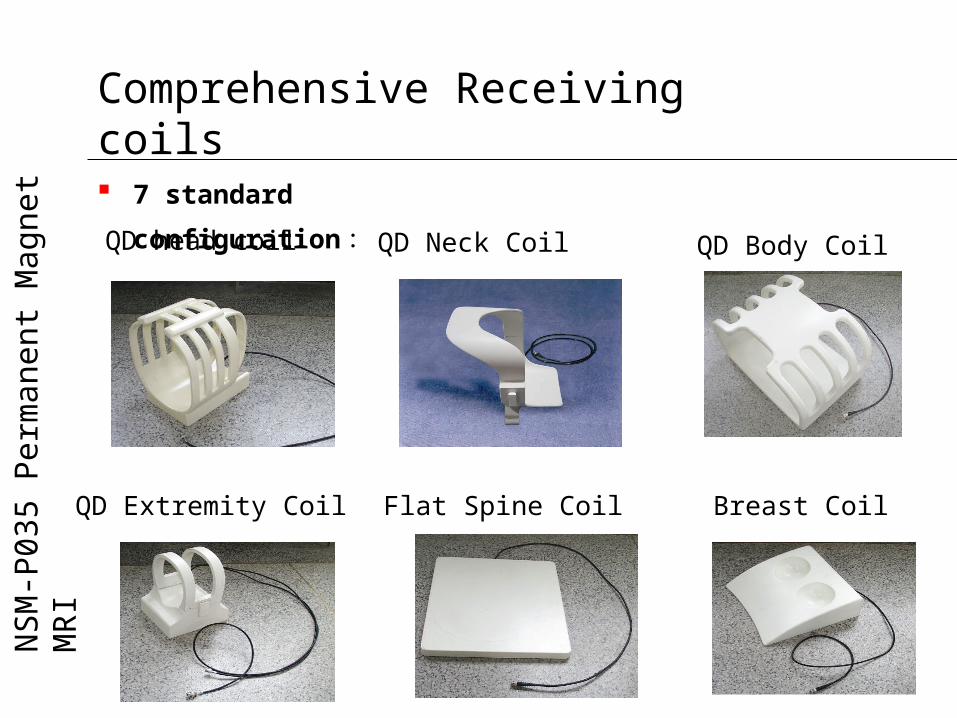
Comprehensive Receiving coils
7 standard configuration:QD head coil QD Neck Coil QD Body Coil
QD Extremity Coil Flat Spine Coil Breast Coil
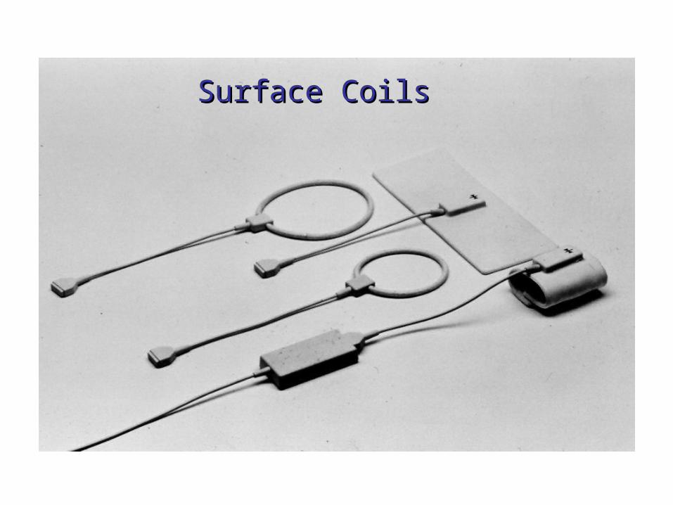
Surface CoilsSurface Coils
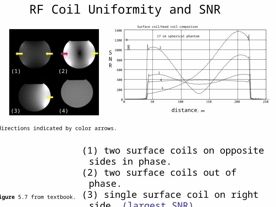
Figure 5.7 from textbook.
SN
R
0 50 100 150 200 2500
200
400
600
800
1000
1200
1400Surface coil/head coil comparison
1
2
3
4
17 cm spherical phantom
distance, mm
b
SNR
(1) two surface coils on opposite sides in phase.(2) two surface coils out of phase.(3) single surface coil on right side. (largest SNR)(4) head coil. (most uniform SNR)
RF Coil Uniformity and SNR
(1) (2)
(3) (4)
B1 directions indicated by color arrows.
Stimulus Presentation / Monitoring
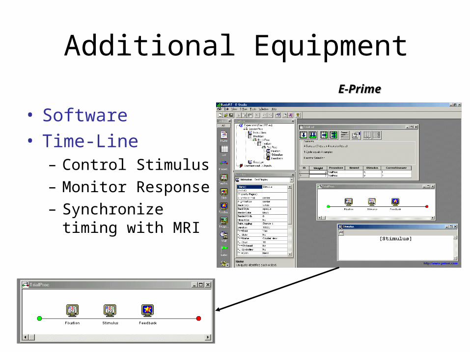
Additional Equipment
• Software• Time-Line
– Control Stimulus
– Monitor Response
– Synchronize timing with MRI
E-PrimeE-Prime
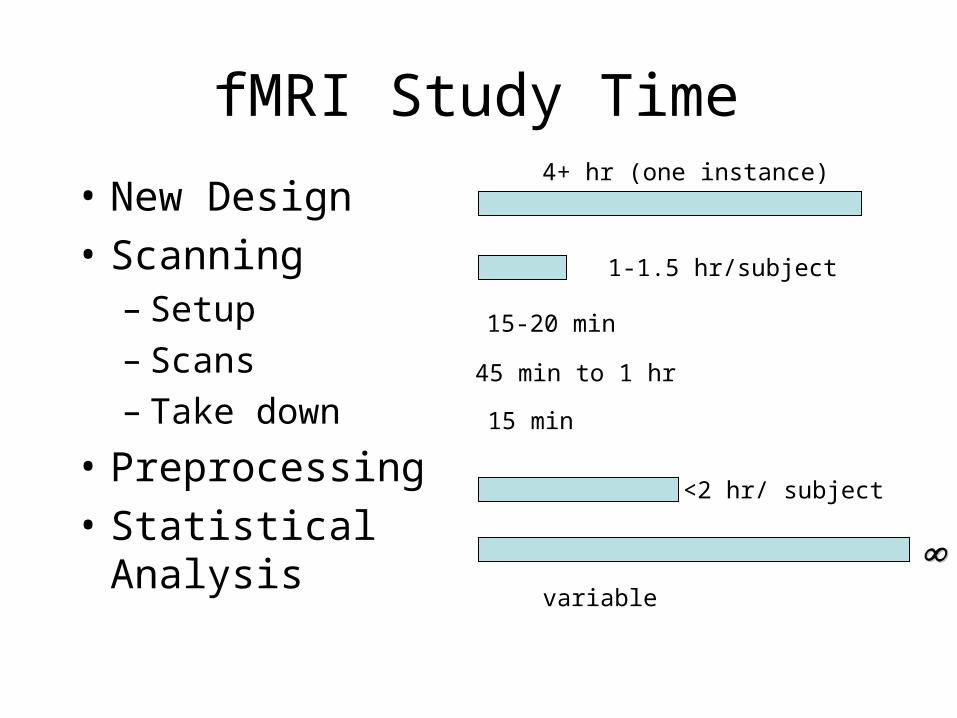
fMRI Study Time
• New Design
• Scanning– Setup– Scans– Take down
• Preprocessing
• Statistical Analysis
1-1.5 hr/subject
4+ hr (one instance)
variable
<2 hr/ subject
15-20 min
45 min to 1 hr
15 min
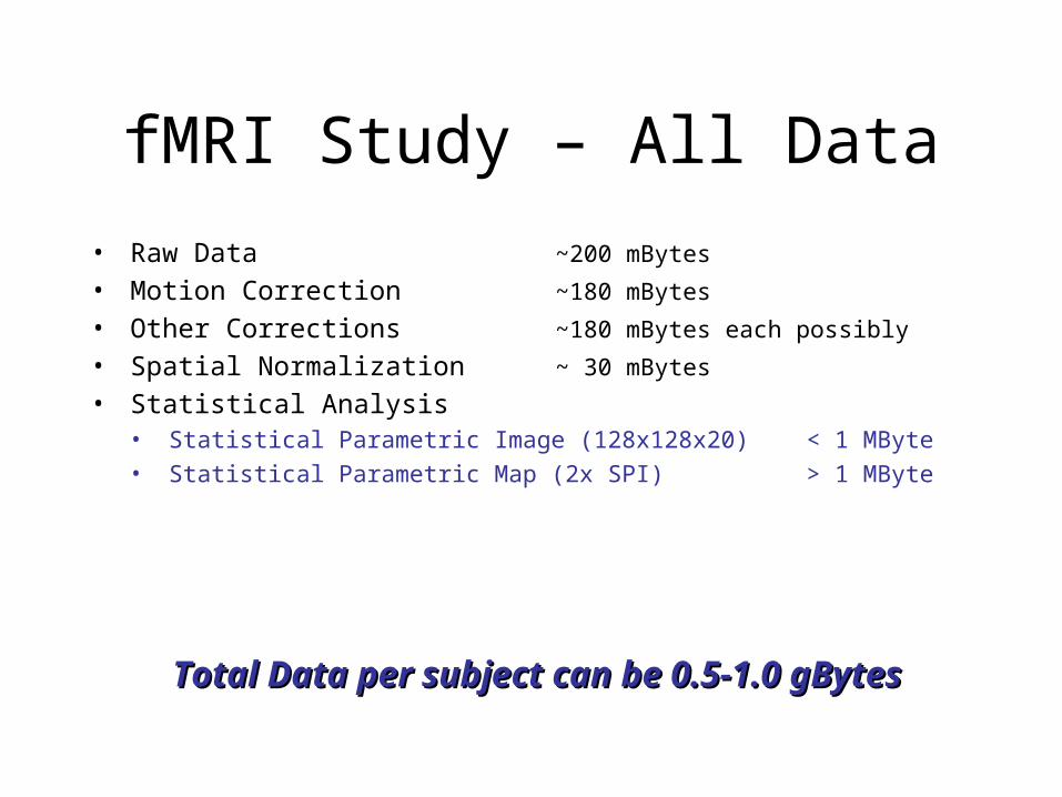
fMRI Study – All Data
• Raw Data ~200 mBytes
• Motion Correction ~180 mBytes
• Other Corrections ~180 mBytes each possibly
• Spatial Normalization ~ 30 mBytes
• Statistical Analysis• Statistical Parametric Image (128x128x20) < 1 MByte
• Statistical Parametric Map (2x SPI) > 1 MByte
Total Data per subject can be 0.5-1.0 gBytesTotal Data per subject can be 0.5-1.0 gBytes
Chapter 7
Spatial and temporal resolution in fMRI
Review
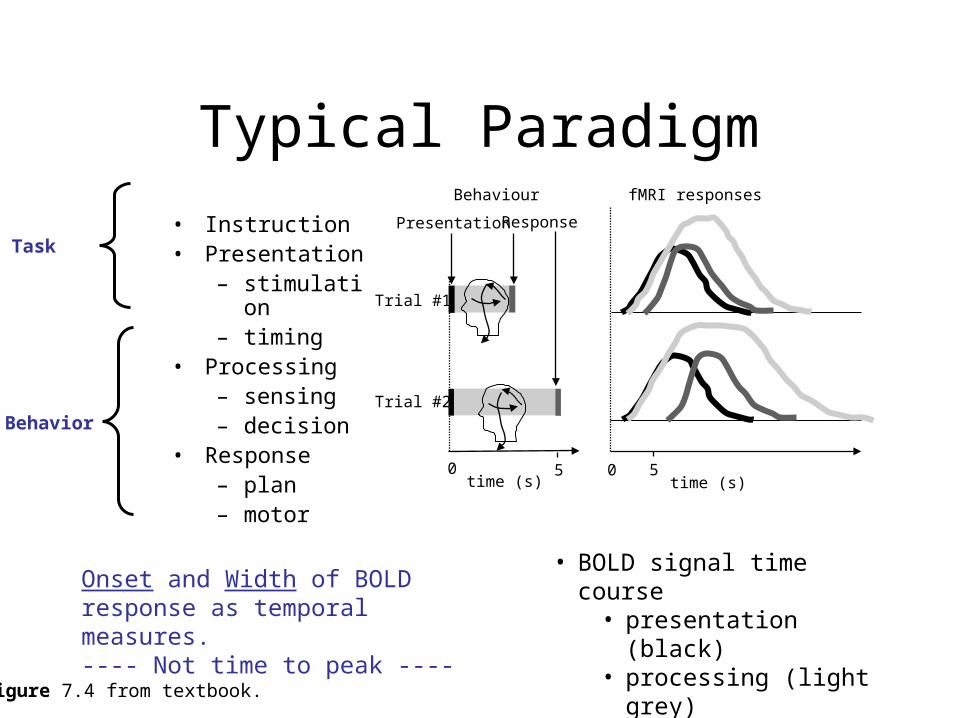
Typical Paradigm
• Instruction• Presentation
– stimulation– timing
• Processing– sensing– decision
• Response– plan– motor
fMRI responses
time (s)
Trial #1
Trial #2
Presentation Response
Behaviour
time (s) 0 5 0 5
Figure 7.4 from textbook.
• BOLD signal time course• presentation (black)• processing (light grey)• response (dark grey)
Task
Behavior
Onset and Width of BOLD response as temporal measures.---- Not time to peak ----
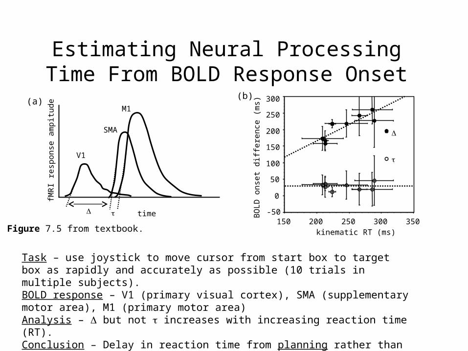
Estimating Neural Processing Time From BOLD Response Onset
V1
SMA
M1
time
fMR
I re
spon
se a
mpi
tude
(a)
350300250200150-50
0
50
100
150
200
250
300
kinematic RT (ms)
BO
LD
ons
et d
iffe
renc
e (m
s)
(b)
Figure 7.5 from textbook.
Task – use joystick to move cursor from start box to target box as rapidly and accurately as possible (10 trials in multiple subjects). BOLD response – V1 (primary visual cortex), SMA (supplementary motor area), M1 (primary motor area)Analysis – but not increases with increasing reaction time (RT).Conclusion – Delay in reaction time from planning rather than execution of movement.
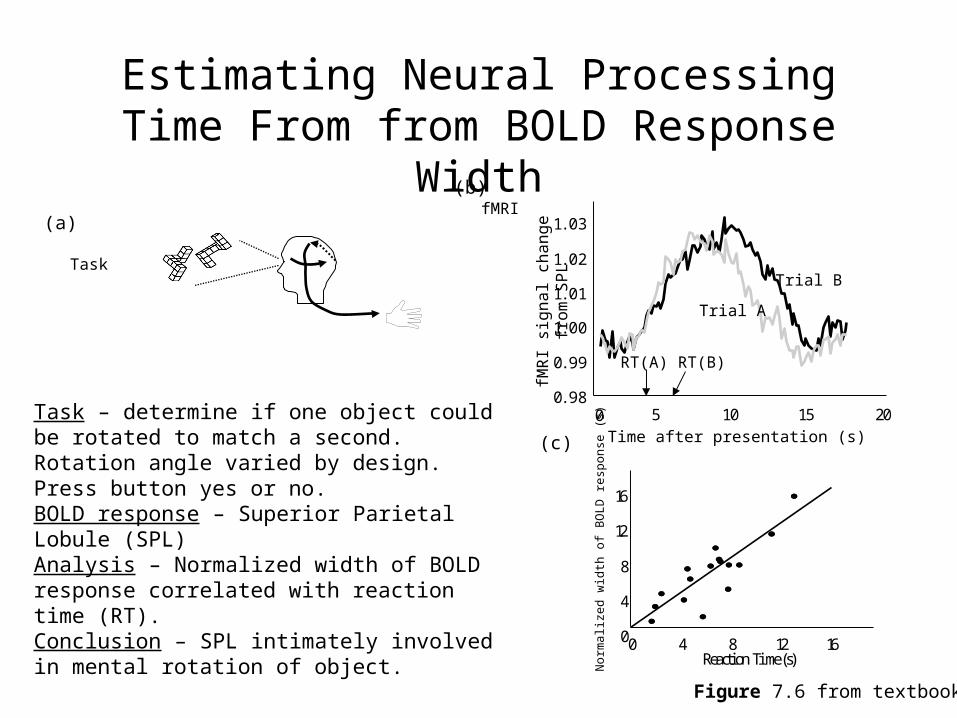
Estimating Neural Processing Time From from BOLD Response Width
fMR
I si
gnal
cha
nge
from
S
PL
Time after presentation (s)
0. 98
0. 99
1. 00
1. 01
1. 02
1. 03fMRI
(b)
20151050
Trial A
Trial B
RT(A) RT(B)
Task
(a)
(c)
16128400
4
8
12
16
Nor
mal
ized
wid
th o
f B
OL
D r
espo
nse
(s)
Reaction Time (s)
Figure 7.6 from textbook.
Task – determine if one object could be rotated to match a second. Rotation angle varied by design. Press button yes or no.BOLD response – Superior Parietal Lobule (SPL)Analysis – Normalized width of BOLD response correlated with reaction time (RT).Conclusion – SPL intimately involved in mental rotation of object.
Chapter 6
Selection of optimal pulse sequences for fMRI
Review
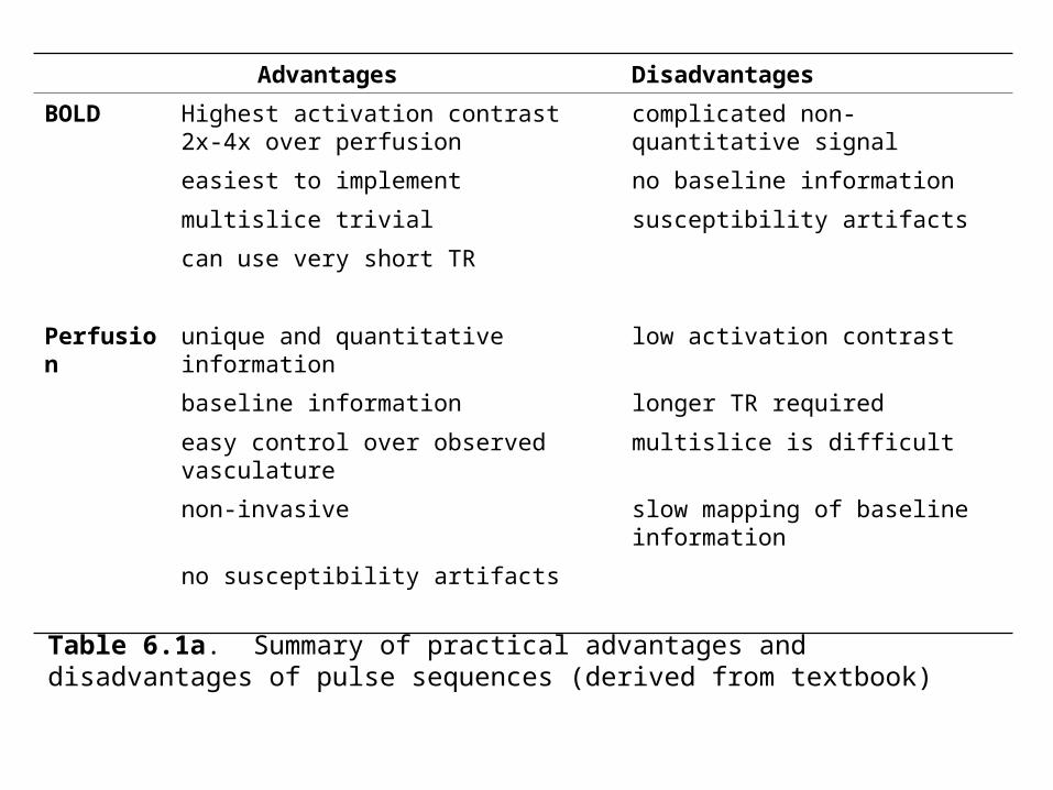
Advantages Disadvantages
BOLD Highest activation contrast 2x-4x over perfusion
complicated non-quantitative signal
easiest to implement no baseline information
multislice trivial susceptibility artifacts
can use very short TR
Perfusion unique and quantitative information low activation contrast
baseline information longer TR required
easy control over observed vasculature multislice is difficult
non-invasive slow mapping of baseline information
no susceptibility artifacts
Table 6.1a. Summary of practical advantages and disadvantages of pulse sequences (derived from textbook)
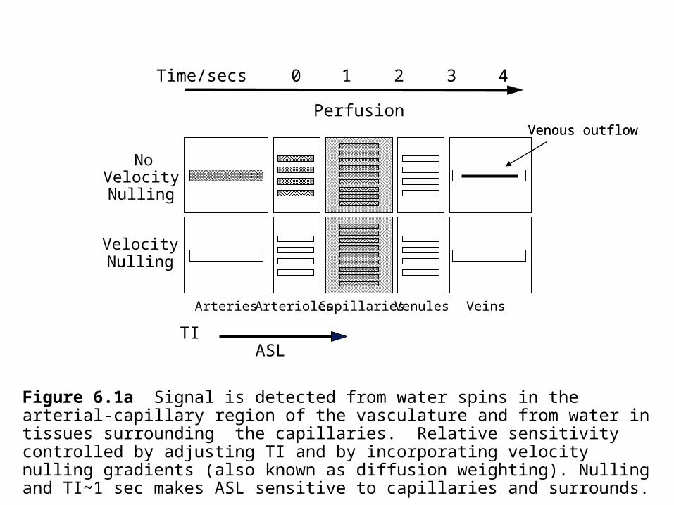
Venous outflow
Perfusion
NoVelocityNulling
VelocityNulling
ASLTI
Time/secs 1 2 40 3
Venous outflow
Figure 6.1a Signal is detected from water spins in the arterial-capillary region of the vasculature and from water in tissues surrounding the capillaries. Relative sensitivity controlled by adjusting TI and by incorporating velocity nulling gradients (also known as diffusion weighting). Nulling and TI~1 sec makes ASL sensitive to capillaries and surrounds.
Arteries Arterioles Capillaries Venules Veins
GE-BOLD
NoVelocityNulling
VelocityNulling
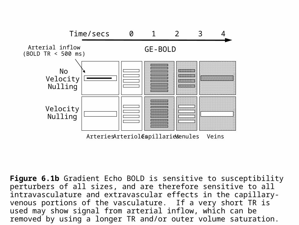
Figure 6.1b Gradient Echo BOLD is sensitive to susceptibility perturbers of all sizes, and are therefore sensitive to all intravasculature and extravascular effects in the capillary-venous portions of the vasculature. If a very short TR is used may show signal from arterial inflow, which can be removed by using a longer TR and/or outer volume saturation.
Arteries Arterioles Capillaries Venules Veins
Arterial inflow(BOLD TR < 500 ms)
Time/secs 1 2 40 3
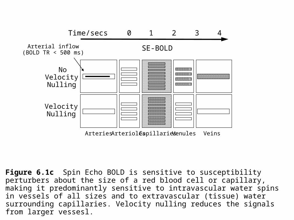
SE-BOLD
NoVelocityNulling
VelocityNulling
Figure 6.1c Spin Echo BOLD is sensitive to susceptibility perturbers about the size of a red blood cell or capillary, making it predominantly sensitive to intravascular water spins in vessels of all sizes and to extravascular (tissue) water surrounding capillaries. Velocity nulling reduces the signals from larger vessesl.
Arteries Arterioles Capillaries Venules Veins
Arterial inflow(BOLD TR < 500 ms)
Time/secs 1 2 40 3
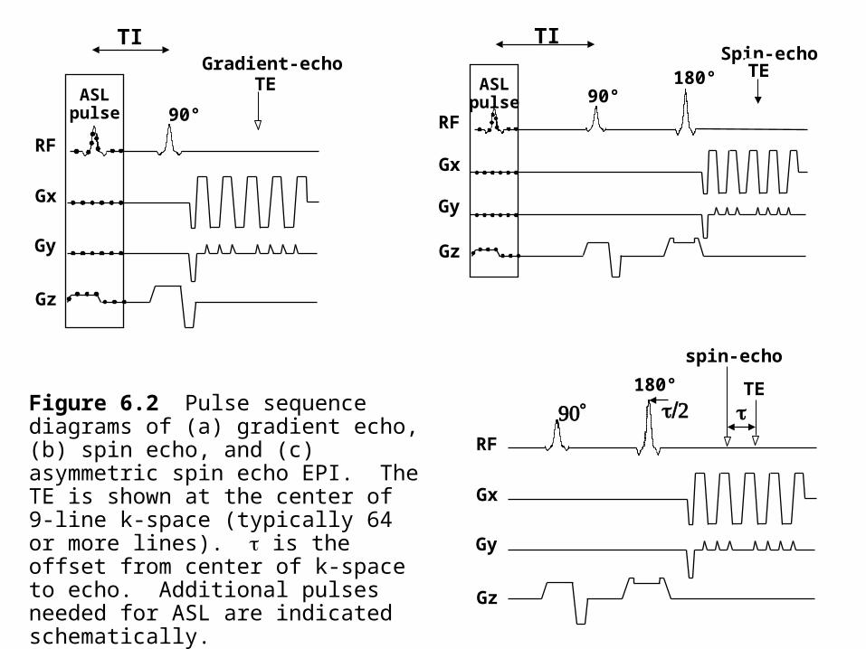
Figure 6.2 Pulse sequence diagrams of (a) gradient echo, (b) spin echo, and (c) asymmetric spin echo EPI. The TE is shown at the center of 9-line k-space (typically 64 or more lines). is the offset from center of k-space to echo. Additional pulses needed for ASL are indicated schematically.
Gradient-echo
RF
Gx
Gz
Gy
90°
TEASLpulse
TISpin-echo
180° TE
RF
Gx
Gz
Gy
ASLpulse
TI
90°
spin-echo
180° TE
RF
Gx
Gz
Gy
Chapter 4
Ultrafast fMRI
Review
Effects of Field Homogeneity
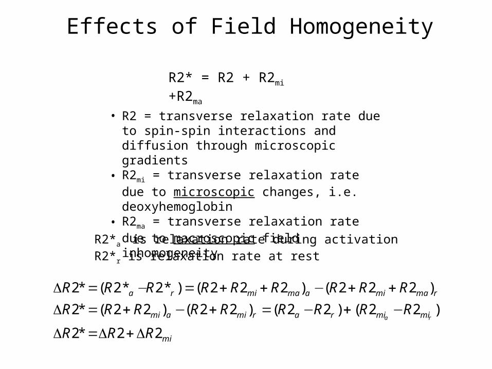
R2* = R2 + R2mi +R2ma
• R2 = transverse relaxation rate due to spin-spin interactions and diffusion through microscopic gradients
• R2mi = transverse relaxation rate due to microscopic changes, i.e. deoxyhemoglobin
• R2ma = transverse relaxation rate due to macroscopic field inhomogeneity
R2*a is relaxation rate during activationR2*r is relaxation rate at rest
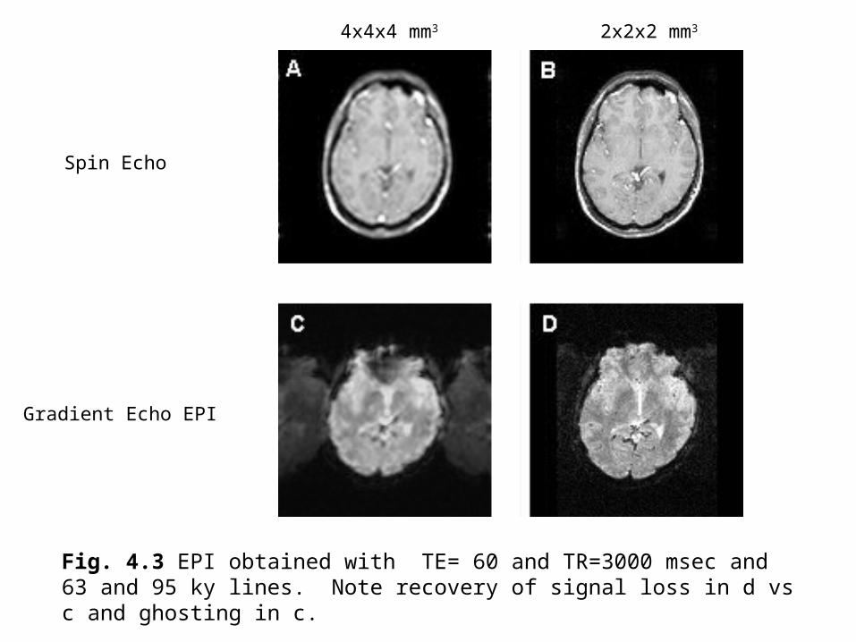
Fig. 4.3 EPI obtained with TE= 60 and TR=3000 msec and 63 and 95 ky lines. Note recovery of signal loss in d vs c and ghosting in c.
Spin Echo
4x4x4 mm3
Gradient Echo EPI
2x2x2 mm3
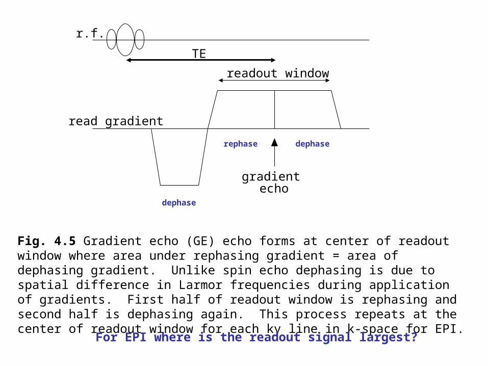
Fig. 4.5 Gradient echo (GE) echo forms at center of readout window where area under rephasing gradient = area of dephasing gradient. Unlike spin echo dephasing is due to spatial difference in Larmor frequencies during application of gradients. First half of readout window is rephasing and second half is dephasing again. This process repeats at the center of readout window for each ky line in k-space for EPI.
gradient echo
readout window
r.f.
read gradient
TE
dephase
rephase dephase
For EPI where is the readout signal largest?
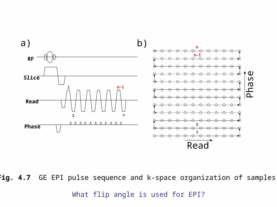
Fig. 4.7 GE EPI pulse sequence and k-space organization of samples.
RF
Slice
Read
Phase
a)
Read
Pha
se
b)
1
2 n
n-1
1
2
n-1
n
What flip angle is used for EPI?
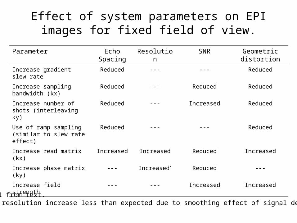
Effect of system parameters on EPI images for fixed field of view.
Parameter Echo Spacing
Resolution SNR Geometric distortion
Increase gradient slew rate Reduced --- --- Reduced
Increase sampling bandwidth (kx)
Reduced --- Reduced Reduced
Increase number of shots (interleaving ky)
Reduced --- Increased Reduced
Use of ramp sampling (similar to slew rate effect)
Reduced --- --- Reduced
Increase read matrix (kx) Increased Increased Reduced Increased
Increase phase matrix (ky) --- Increased* Reduced ---
Increase field strength --- --- Increased Increased
Table 4.1 from text. * actual resolution increase less than expected due to smoothing effect of signal decay.
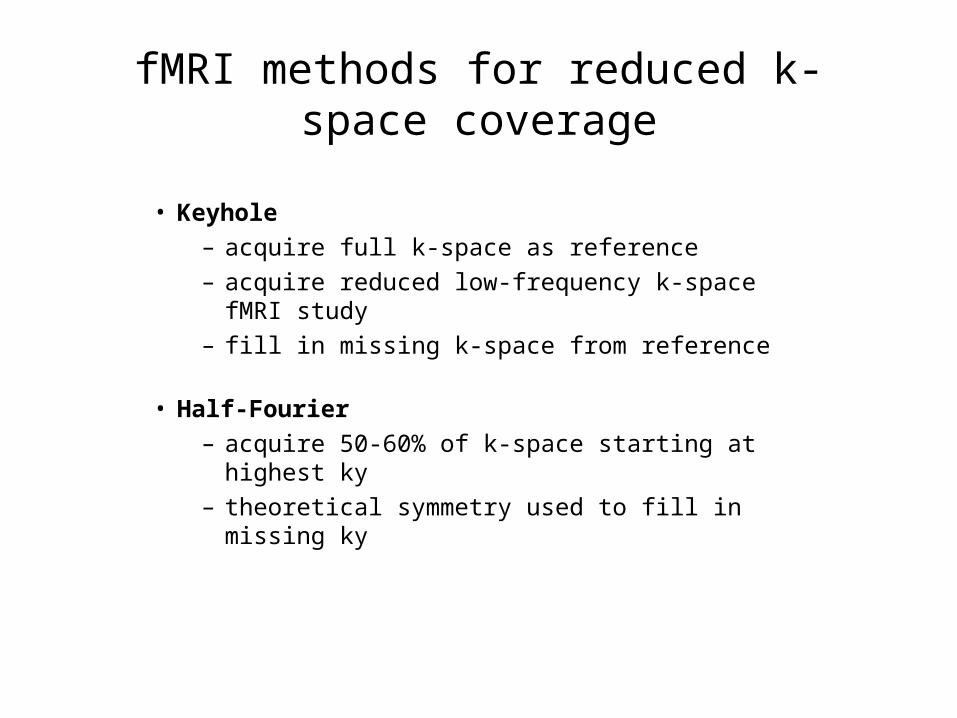
fMRI methods for reduced k-space coverage
• Keyhole
– acquire full k-space as reference
– acquire reduced low-frequency k-space fMRI study
– fill in missing k-space from reference
• Half-Fourier
– acquire 50-60% of k-space starting at highest ky
– theoretical symmetry used to fill in missing ky
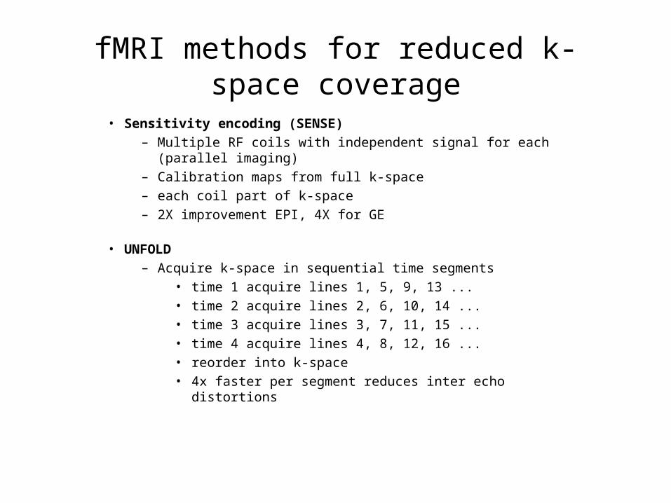
fMRI methods for reduced k-space coverage
• Sensitivity encoding (SENSE)– Multiple RF coils with independent signal for each (parallel imaging)– Calibration maps from full k-space– each coil part of k-space– 2X improvement EPI, 4X for GE
• UNFOLD– Acquire k-space in sequential time segments
• time 1 acquire lines 1, 5, 9, 13 ...• time 2 acquire lines 2, 6, 10, 14 ...• time 3 acquire lines 3, 7, 11, 15 ...• time 4 acquire lines 4, 8, 12, 16 ...• reorder into k-space• 4x faster per segment reduces inter echo distortions


