30
Chapter 3 Data Exploration and Dimension Reduction 1
| Date post: | 26-Dec-2015 |
| Category: |
Documents |
| Upload: | jared-webster |
| View: | 228 times |
| Download: | 4 times |

Chapter 3
Data Exploration and
Dimension Reduction
1

Introduction• Large number of variables in the database.
– Likely that subsets of variables are highly correlated with each other– Variables that are unrelated to the outcome of interest– In a classification or prediction model leads to over fitting – Accuracy and reliability can suffer. – Large numbers of variables also pose computational problems for some
models (aside from questions of correlation.) – In model deployment, superfluous variables can increase costs due to
collection and processing of these variables.
• “Dimensionality" of a model is the number of independent or input variables used by the model.
• Key step in data mining – Find ways to reduce dimensionality without sacrificing accuracy
2

Practical Considerations• First step of data exploration
– Make sure that the measured variables are reasonable for the task
• Integration of expert knowledge through a discussion with the data provider will lead to better results.
• Practical considerations – Which variables are most important and – Which are most likely to be useless for the task at hand? – Which variables are likely to contain much error? – Which variables will be available for measurement (and their cost
feasibility) in the future, if the analysis will be repeated? – Which variables can actually be measured before the outcome occurs?
• Example, if we want to predict the closing price of an auction, we cannot use the number of bids as a predictor, because this is unknown until the auction closes
3

4

Data Summaries
5

Data Summaries
6

Data Summaries
7

Data Visualization
8

Data Visualization
9

Correlation Analysis• Datasets with a large number of variables
– Usually much overlap in the information covered by the set of variables.
• Find redundancies– Look at a correlation matrix– Shows all the pairwise correlations between the variables
• Pairs that have a very strong (positive or negative) correlation – Contain overlap in information– Good candidates for data reduction by removing one of the variables. – Avoids multicollinearity
• Multicollinearity is the presence of two or more predictors sharing the same linear relationship with the outcome variable
10

• Correlation matrix method used to find variable duplications in the data– Sometimes the same variable accidently appears more than once in
the dataset (under a different name) because the dataset was merged from multiple sources
– The same phenomenon is measured in different units, etc.
– Using color to encode the correlation magnitude in the correlation matrix can make the task of identifying strong correlations easier.
11
Correlation Analysis

Reducing the Number of Categories in Categorical Variables
• When a categorical variable has many categories, and this variable is destined to be a predictor, it will result in many dummy variables.
• A variable with m categories will be transformed into variables m - 1 dummy variables when used in an analysis.
• Categorical variables can greatly inflate the dimension of the dataset. • Reduce the number of categories by binning close bins together. • Requires incorporating expert knowledge and common sense. • Pivot tables are useful for this task:
– We can examine the sizes of the different categories and how the response behaves at each category.
• Bins that contain very few observations are good candidates for combining with other categories. – Use only the categories that are most relevant to the analysis– Label the rest as “other.”
12

Principal Components Analysis • Principal components analysis (PCA) is a useful procedure for
reducing the number of predictors in the model by analyzing the input variables.
• Assumes we have subsets of measurements – That are measured on the same scale – And are highly correlated
• Provides a few variables (often as few as three) that are weighted linear combinations of the original variables
• Retain the explanatory power of the full original set– Explanatory value in terms of variance
• PCA is intended for use with quantitative variables• For categorical variables use other methods
– Such as correspondence analysis13

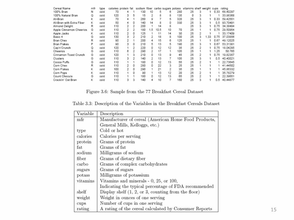
Example: Breakfast Cereals
14
15

16

Covariance & Correlation
17

The Principal Components• The idea in PCA is to find a linear combination of the two variables that
contains most of the information• This new variable can replace the two original variables• Information is variability
– what can explain the most variability among the 77 cereals? – Total variability here is the sum of the variances of the two variables(379.63 +
197.32 = 577– Calories account for 66% = 379.63/577 of the total variability, – Rating for the remaining 44%.
• Drop one of the variables for the sake of dimension reduction, then we lose at least 44% of the total variability.
• Can we redistribute the total variability between two new variables in a more polarized way?
• If so, then it might be possible to keep only the one new variable that accounts for (hopefully) a large portion of the total variation.
18

• Figure 3.7 shows the scatter plot of Rating vs. Calories. • The line z1 is the direction in which the variability of the points is largest. • It is the line that captures the most variation in the data if we decide to reduce the
dimensionality of the data from two to one. • Among all possible lines, it is the line for which, if we project the points in the
dataset orthogonally to get a set of 77 (one dimensional) values, the variance of the z1 values will be maximum.
• This is called the first principal component. • It is also the line that minimizes the sum of squared perpendicular distances from
the line. • The z2 axis is chosen to be perpendicular to the z1 axis. • In the case of two variables there is only one line that is perpendicular to z1, and it
has the second largest variability, but its information is uncorrelated with z1. • This is called the second principal component. • In general, when we have more than two variables, once we find the direction z1
with the largest variability, we search among all the orthogonal directions to z1 for the one with the next highest variability.
• That is z2. The idea is then to find the coordinates of these lines, and to see how they redistribute the variability.
19
The Principal Components

20

• Figure 3.8 shows the XLMiner output from running PCA on these two variables. • The Principal Components table gives the weights that are used to project the original points
onto the two new directions. • The weights for z1 are given by (-0.847, 0.532), and for z2 they are given by (0.532, 0.847). • The table below gives the new reallocated variation: z1 accounts for 86% of the total
variability and the remaining 14% are accounted by z2. Therefore, if we drop z2 we still maintain 88% of the total variability.
• The weights are used to compute principal component scores, which are the projected values of Calories and Rating onto the new axes (after subtracting the means).
21
The Principal Components

• Figure 3.9 shows the scores for the two dimensions. • The first column is the projection onto z1 using the weights (-0.847, 0.532). • The second column is the projection onto z2 using the weights (0.532, 0.847). • For instance, the first score for the 100% Bran cereal (with 70 calories and
rating of 68.4) is (-0.847)(70 – 106.88) + (0.532)(68.4 – 42.67) = 44.92. • Notice that the means of the new variables z1 and z2 are zero (because we've
subtracted the mean of each variable). • The sum of the variances var(z1) + var(z2) is equal to the sum of the variances
of the original variables, Calories and Rating. • Furthermore, the variances of z1 and z2 are 498 and 79 respectively, so the
first principal component, z1, accounts for 86% of the total variance. • Since it captures most of the variability in the data, it seems reasonable to use
one variable, the first principal score, to represent the two variables in the original data.
22
The Principal Components

23

24

Normalizing the Data• Before PCA normalize data• Normalization (or standardization) means replacing each
original variable by a standardized version of the variable that has unit variance. – Accomplished by dividing each variable by its standard deviation.
• The effect of this normalization (standardization) is to give all variables equal importance in terms of the variability
• We perform PCA on the covariance matrix. • An alternative is to perform PCA on the correlation matrix
instead of the covariance matrix • Most software programs allow the user to choose between
the two• Using the correlation matrix means that you are operating on
the normalized data.
25

26

The Principal Components• We normalized the 13 variables due to the different scales of the variables, and
then perform PCA (or equivalently, we use PCA applied to the correlation matrix).
• We need find the principal components to account for more than 90% of the total variability.
• The first two principal components account for only 52% of the total variability, – reducing the number of variables to two would mean loosing a lot of information.
• Examining the weights, – the first principal component measures the balance between two quantities: – (1) calories and cups (large positive weights) vs. (2) protein, fiber, potassium, and consumer
rating (large negative weights).
• High scores on principal component 1 mean that the cereal is high in calories and the amount per bowl, and low in protein, fiber, and potassium. – This type of cereal is associated with low consumer rating.
• The second principal component is most affected by the weight of a serving• The third principal component by the carbohydrate content.
27

28

Using Principal Components for Classification and Prediction
• The goal of data reduction is to have a smaller set of variables that will serve as predictors
• We can proceed as following: – Apply PCA to the training data.
• Use the output to determine the number of principal components to be retained.
• The predictors in the model now use the (reduced number of) principal scores columns.
– For the validation set • We can use the weights computed from the training data to
obtain a set of principal scores, • Apply the weights to the variables in the validation set. • These new variables are then treated as the predictors.
29

Problems
• 3.2 Breakfast Cereals
• 3.5 Sales of Toyota Cars
30


