105
Communication “PCM – TDM – PSTN – Data Traffic Engineering” Dr. Cahit Karakuş, 2019 1
Communication
“PCM – TDM – PSTN – Data Traffic Engineering”
Dr. Cahit Karakuş, 2019
1

İçerik
• Ses Dalgaları
• Pulse Code Modulation
• TDM – E1
• PSTN: Public Switched Telephone Network
• Data Traffic Engineering
2

3
Ses Dalgaları

Ses
• Ses havada ses dalgaları (Mekanik) ile yayılır.
• Sesin havada ortalama yayılma hızı=342 m/s. Yayılma hızı hava sıcaklığı ve diğer koşullara bağlı olarak değişim gösterir.
• Ses dalgaları boşlukta yayılmaz. Görsel köpürür…
4

Ses dalgaları 4’e ayrılır
• Ses ötesi (Infrasound); 20 hertz ve altındaki ses dalgalardır.
• İşitilebilir ses; 20-20 000 hertz arasında olan ses dalgalardır.
• Ultra ses (Ultrasound); 20KHz (20.000 hertz) den 15MHz’e kadar olan ses dalgalarıdır. Bu dalgalar anne karnında bebek görüntüleme ve böbrek taşı kırmada kullanılır.
• Hiperses(Hypersound): frekansları 15MHz’den yukarı olan ses dalgalarıdır.
5
İnsan Kulağı
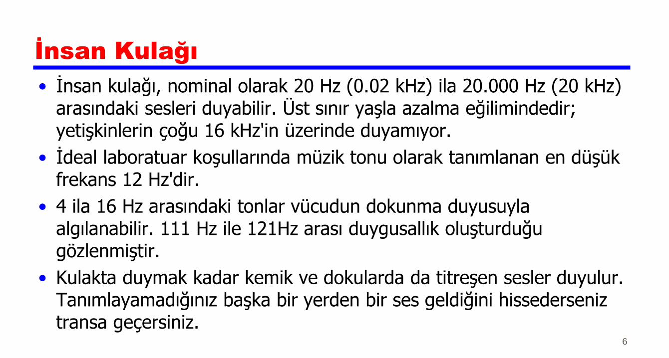
• İnsan kulağı, nominal olarak 20 Hz (0.02 kHz) ila 20.000 Hz (20 kHz) arasındaki sesleri duyabilir. Üst sınır yaşla azalma eğilimindedir; yetişkinlerin çoğu 16 kHz'in üzerinde duyamıyor.
• İdeal laboratuar koşullarında müzik tonu olarak tanımlanan en düşük frekans 12 Hz'dir.
• 4 ila 16 Hz arasındaki tonlar vücudun dokunma duyusuyla algılanabilir. 111 Hz ile 121Hz arası duygusallık oluşturduğu gözlenmiştir.
• Kulakta duymak kadar kemik ve dokularda da titreşen sesler duyulur. Tanımlayamadığınız başka bir yerden bir ses geldiğini hissederseniz transa geçersiniz.
6

Konuşmanın Bileşenleri
• Sesin işitme frekans aralığı, 20Hz-16kHz dir. Konuşma 100Hz-7kHz aralığındadır.
• Ses dalgaları mikrofon yardımıyla elektriksel analog sinyale dönüştürülür. Peryodik
sinyallerden oluşur. İletim için kolayca elektromanyetik sinyale dönüştürülür
• Ses frekansları, değişen frekans ve voltaja sahip elektromanyetik frekanslara dönüştürülür.
• Sesin sınır frekans aralığı: Tanıma, Anlama, Hissetme özelliklerini sağlar: 300-3400Hz
• Ses, elektrik sinyale dönüşür. Analog sinyalin karekteristikleri: Genlik, frekans ( f ), Dalga boyu ( λ ), Faz
7

Lifecycle from Sound to Digital
to Sound
Source: http://en.wikipedia.org/wiki/Digital_audio

Introduction
What is Speech Coding ?

10
Pulse Code Modulation

ANALOG-TO-DIGITAL CONVERSION
A digital signal is superior to an analog signal because it is more robust (güçlü) to noise and can easily be
recovered, corrected and amplified. For this reason, the tendency (eğilim) today is to change an analog signal
to digital data.
Dijital bir sinyal analog sinyale göre daha üstündür çünkü ekonomiktir, gürültüye karşı daha dayanıklıdır ve
kolayca geri kazanılabilir, düzeltilebilir ve yükseltilebilir. Bu sebeple, günümüzdeki eğilim bir analog sinyali
dijital verilere değiştirmektir. Bilgisayar ya da sayısal sistemlerden bahsedilmektedir. İletim ortamında sayısal
sinyal elverişli değildir.

PCM
PCM consists of three steps to digitize an analog signal:
1. Sampling
2. Quantization
3. Binary encoding
Before we sample, we have to filter the signal to limit the maximum frequency of the signal as it affects the sampling rate.
Filtering should ensure that we do not distort the signal, remove high frequency components that affect the signal shape.

Nyquist Sampling Theorem
For lossless digitization, the sampling rate should be at least twice the maximum frequency response. Sayısal iletim ortamının performansını belirler.
• In mathematical terms:
fs ≥ 2*fm
fs ≥ 2*B
• where fs is sampling frequency and fm is the maximum frequency in the signal; B is the bandwidth. Birimleri Hz=1/sec. Frekans bir saniyedeki titreşim sayısıdır.
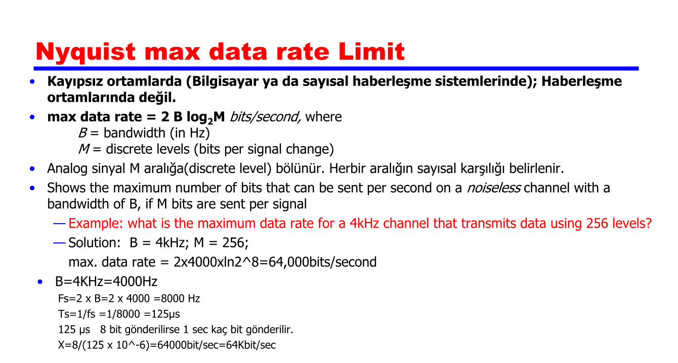
Nyquist max data rate Limit • Kayıpsız ortamlarda (Bilgisayar ya da sayısal haberleşme sistemlerinde); Haberleşme
ortamlarında değil.
• max data rate = 2 B log2M bits/second, where B = bandwidth (in Hz) M = discrete levels (bits per signal change)
• Analog sinyal M aralığa(discrete level) bölünür. Herbir aralığın sayısal karşılığı belirlenir.
• Shows the maximum number of bits that can be sent per second on a noiseless channel with a bandwidth of B, if M bits are sent per signal
— Example: what is the maximum data rate for a 4kHz channel that transmits data using 256 levels?
— Solution: B = 4kHz; M = 256;
max. data rate = 2x4000xln2^8=64,000bits/second
• B=4KHz=4000Hz Fs=2 x B=2 x 4000 =8000 Hz
Ts=1/fs =1/8000 =125µs
125 µs 8 bit gönderilirse 1 sec kaç bit gönderilir.
X=8/(125 x 10^-6)=64000bit/sec=64Kbit/sec

Shannon’s Theorem
• Shannon’s theorem gives the capacity of a system in the presence of noise. Analog iletim ortamının kapasitesini belirler.
C = B log2(1 + SNR)
The Shannon capacity gives us the upper limit; the Nyquist formula tells us how
many signal levels we need.
15

Sampling
•
Sampling usually happens at equally separated intervals; this interval is called the sampling interval. The reciprocal of sampling interval is called the sampling frequency or sampling rate. The unit of sampling rate is Hz Örnekleme genellikle eşit zaman aralıklarında yapılır; bu aralığa örnekleme aralığı denir. Örnekleme aralığının karşılığına örnekleme frekansı veya örnekleme oranı denir. Örnekleme oranı birimi Hz
• In agreement with the sampling theorem, the telephone audio signals (with frequency between 300 Hz to 3400 Hz; it is taken 4KHz), should be sampled at a frequency equal or greater than 6800 Hz (8000Hz). Actually, we usually take the sampling frequency or sampling rate at 8000 Hertz. Bir analog sinyalden saniyede eşit aralıklarla 8000 örnek alınıyor ve bir örnekleme 8 bit ile temsil ediliyorsa saniyde kaç bit örnek alınır? 8000 x 8=64 000 bit/sec=64Kbit/sec.
• Herbir örnek 8 bit ile temsil ediliyor ise, örnekleme aralık sayısı (Kuantalama) 2^8=256 dır. T=1/8000= 0.000125 sec. = 125 µs , T örnekleme aralığıdır.

Signal Sampling
• Sampling is converting a continuous time signal into a discrete time signal
• Categories:
—Impulse (ideal) sampling
—Natural Sampling
—Sample and Hold operation

Ideal Sampling and Aliasing
• Sampled signal is discrete in time domain with spacing Ts
• Spectrum will repeat for every fs Hz
• Aliasing (spectral overlapping) if fs is too small (fs < 2fm)
• Nyquist sampling rate fs = 2fm
• Generally oversampling is done fs > 2fm

Concepts
Quantalama

NON-LİNEER QUANTALAMA
• Lineer quantalama sisteminde düşük genlikli
sinyallerin hata oranı yüksek olur.
• Telefonda kısık sesli konuşanların seslerinin
büyük kısmı kaybolur. Bunu önlemek için
genlik eksenini parçalara bölerken eşit
bölünmez.
• Düşük genlikli sinyallerde aralıklar daha sık
yüksek genlikli sinyallerde aralıklar daha
seyrektir.
• Aralıklar öyle ayarlanır ki sinyal gürültü oranı
hep aynı olur. Bu işleme non-lineer
quantalama denir.
•
2Mbit/sn Frame Çerçevesinin Oluşturulması

NON-LİNEER QUANTALAMA
28 = 256 Adet işareti kodlayabiliriz.
1. 1.Bit pozitif veya negatif bölgeyi gösterir.
1 olursa pozitif bölge
0 olursa negatif bölge
2. 2,3,4. Bitler hangi parçada bulunduğunu gösterir.(010)
3. 5,6,7,8. Bitler parça içinde bulunduğu yeri gösterir.
Bu dört karekterle 16 ayrı kodlama yapabiliriz.
Görüldüğü her parçada 15 adet kodlama vardır.
ÖRNEK: Pozitif 2.parçada 45 in kodlaması nasıl yapılır?
1 0 1 0 1 1 0 1
2Mbit/sn Frame Çerçevesinin Oluşturulması
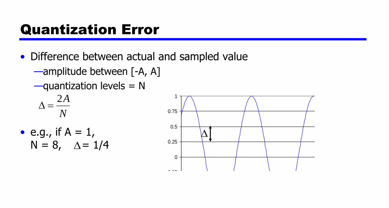
Quantization Error
• Difference between actual and sampled value
—amplitude between [-A, A]
—quantization levels = N
• e.g., if A = 1, N = 8, = 1/4
N
A2
-1
-0.75
-0.5
-0.25
0
0.25
0.5
0.75
1
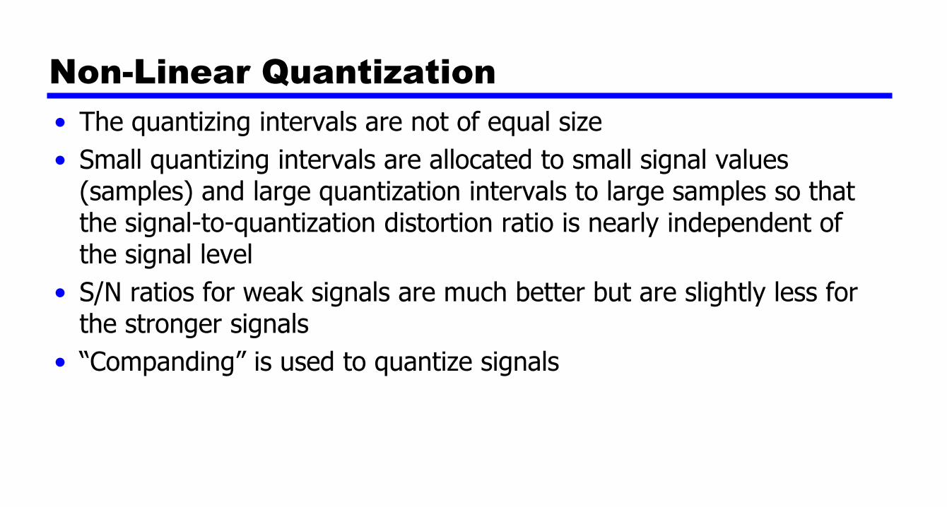
Non-Linear Quantization
• The quantizing intervals are not of equal size
• Small quantizing intervals are allocated to small signal values (samples) and large quantization intervals to large samples so that the signal-to-quantization distortion ratio is nearly independent of the signal level
• S/N ratios for weak signals are much better but are slightly less for the stronger signals
• “Companding” is used to quantize signals

Pulse Code Modulation Standarts
• PCM is a Time-Domain Waveform coding method and is defined within CCITT G.711, and AT&T 43801. Basically, an analog signal is sampled at a rate of 8000 times per second. In each sample, the amplitude of the signal is assigned (quantized) a digital value.
• There are two PCM algorithms defined within CCITT G.711, called "A-Law" and "Mu-Law". Mu-Law PCM is used in North America and Japan, and A-Law used in most other countries. In both A-Law and Mu-Law PCM, the values used to represent the amplitude is a number between 0 and +/- 127; therefore, 8 bits are required to represent each sample (2 to the eigth power = 256).
• It can be seen then that PCM operates at a rate of: 8 bits/sample * 8000 samples/sec = 64000 (64K) Bits Per Second.

Components of PCM encoder

Three different sampling methods for PCM

We want to digitize (ayrık) the human voice. What is the bit rate, assuming 8
bits per sample?
Solution
The human voice normally contains frequencies from 0 to 4000 Hz. So the
sampling rate and bit rate are calculated as follows:
Example

The process of delta modulation

Adaptive Differential PCM (ADPCM)
• Adaptive Differential Pulse Code Modulation (ADPCM) codecs are waveform codecs which instead of quantizing the speech signal directly, quantize the difference between the speech signal and a prediction that has been made of the speech signal.
• If the prediction is accurate then the difference between the real and predicted speech samples will have a lower variance than the real speech samples, and will be accurately quantized with fewer bits than would be needed to quantize the original speech samples.

Companding
• Formed from the words compressing and expanding.
• A PCM compression technique where analogue signal values are rounded on a non-linear scale.
• The data is compressed before sent and then expanded at the receiving end using the same non-linear scale.
• Companding reduces the noise and crosstalk levels at the receiver.

Speech Compression Standards • 64 kbps µ-law/A-law PCM(CCTT G.711)
• 32 kbps ADPCM(CCITT G.721)
• 16 kbps Low Delay CELP(CCITT G.728)
• 13.2 kbps RPE-LTP(GSM 06.10)
• 13 kbps ACELP(GSM 06.60)
• 13 kbps QCELP(US CDMA Cellular)
• 8 kbps QCELP(US CDMA Cellular)
• 8 kbps VSELP(US TDMA Cellular)
• 8 kbps CS-ACELP(ITU G.729)
• 6.7 kbps VSELP(Japan Digital Cellular)
• 6.4 kbps IMBE(Immarsat Voice Coding Standard)
• 5.3 & 6.4 kbps True Speech Coder(ITU G.723)
• 4.8 kbps CELP(Fed. Standard 1016-STU-3)
• 2.4 kbps LPC(Fed. Standard 1015 LPC-10E)

“Circuit Switching
PSTN”
Dr. Cahit Karakuş, 2019

33
PSTN Public Switched Telephone Network
History and Evolution of
circuit switching - PSTN
—Manual, Strowger, register, cross bar system, trunking, electronic and digital switching systems

PSTN
Users
Local
Telephone
Exchanges
City Telephone
Exchange
Traffic from 1
user
Traffic from all
users connect
to exchange
Traffic from all
local exchanges
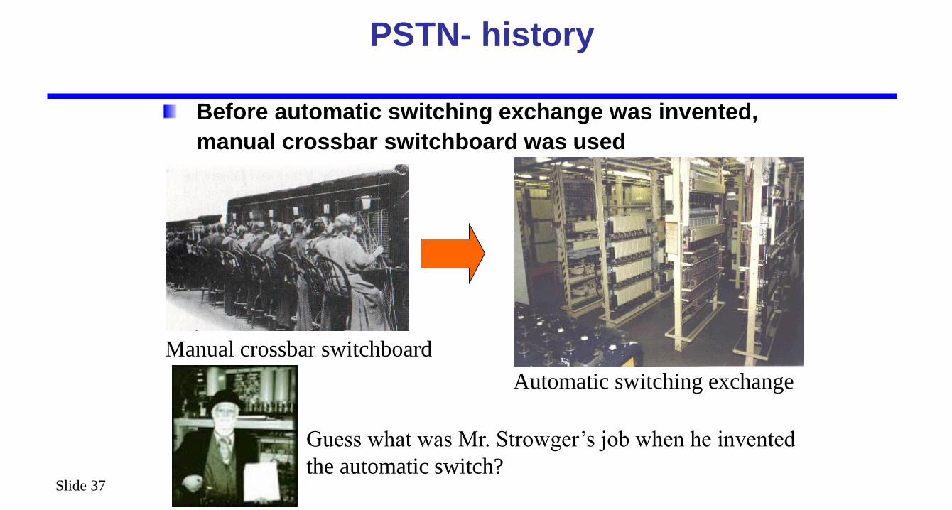
Slide 37
Before automatic switching exchange was invented,
manual crossbar switchboard was used
PSTN- history
Manual crossbar switchboard
Automatic switching exchange
Guess what was Mr. Strowger’s job when he invented
the automatic switch?
Slide 38
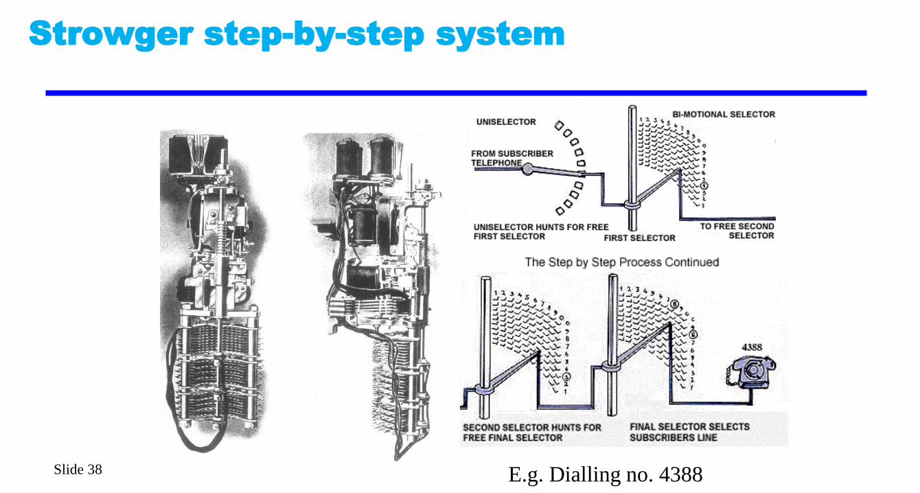
Strowger step-by-step system
E.g. Dialling no. 4388

Slide 39
•Public Switched Telephone
Network (PSTN) consists of
switching nodes (called
exhanges) in hierarchical
structure:
(a) Local network – connect customers’ stations to LEs
(b) Junction network – interconnect group of LEs
(c) Trunk / toll network – provides long distance circuits within country
(d) International network – provide circuits between countries
Public Switched Telephone Network (PSTN)

40

Public Circuit Switched Network

Structure of the PSTN
• Switching
• Transport or transmission (PDH, SDH)
• Subscriber signalling (analog or digital)
• Network-internal signalling (SS7)
• Intelligent Network (IN) concept
• Basic components also for circuit-switched core of mobile networks (PLMN)

Slide 43
•Time-division multiplexing (TDM) transmission was initially
introduced for trunk and junction circuits in the form of
pulse-code modulation (PCM).
•If TDM transmission is used with space-division tandem
switching, it is necessary to provide demultiplexing of
PCM channels to audio signals before switching and
multiplexing of audio signals into PCM channels after
switching for retransmission.
Digital Switching Systems

Slide 44
•There are no customer lines involved in tandem exchanges
– no disadvantage of high-cost customers’ lines.
•Thus, digital exchanges were first introduced for trunk and
junction switching.
•This led to the conversion of trunk networks into integrated
digital networks (IDN) – digital transmission and switching.
Digital switching systems: trunk & junction switch
Slide 45
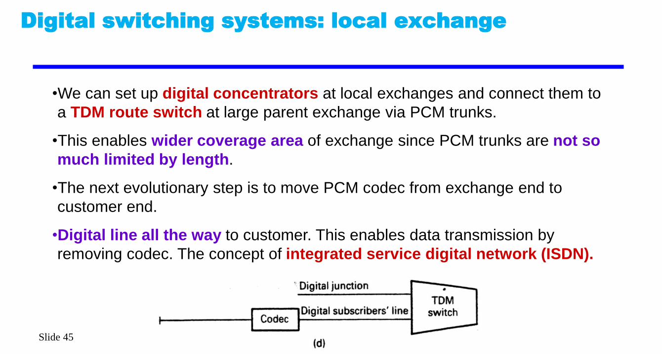
•We can set up digital concentrators at local exchanges and connect them to
a TDM route switch at large parent exchange via PCM trunks.
•This enables wider coverage area of exchange since PCM trunks are not so
much limited by length.
•The next evolutionary step is to move PCM codec from exchange end to
customer end.
•Digital line all the way to customer. This enables data transmission by
removing codec. The concept of integrated service digital network (ISDN).
Digital switching systems: local exchange

Basic local exchange (LE) architecture
Time switch
TDM links to other network elements
• Switch control
Switching system
• E.164 number analysis
• Charging
• User databases
LIC
LIC
Tone Rx
Group switch
Sign.
ETC
ETC
Exchange terminal circuit
Line interface circuit
SS7 Signalling equipment
Control system • O&M functions
Subscriber stage
Modern trend: Switching and control functions are separated into different network elements (separation of user and control plane).
Tone generator

Setup of a call (1)
Time switch
2. Check user database. For instance, is user A barred for outgoing calls?
Switching system
3. Reserve memory for user B number
LIC
LIC
Tone Rx
Group switch
Sign.
ETC
ETC
Control system
Phase 1. User A lifts handset and receives dial tone.
1. Off hook
Local exchange of user A
4. Tone Rx is connected
5. Dial tone is sent (indicating “network is alive”)
Tone generator
Time switch
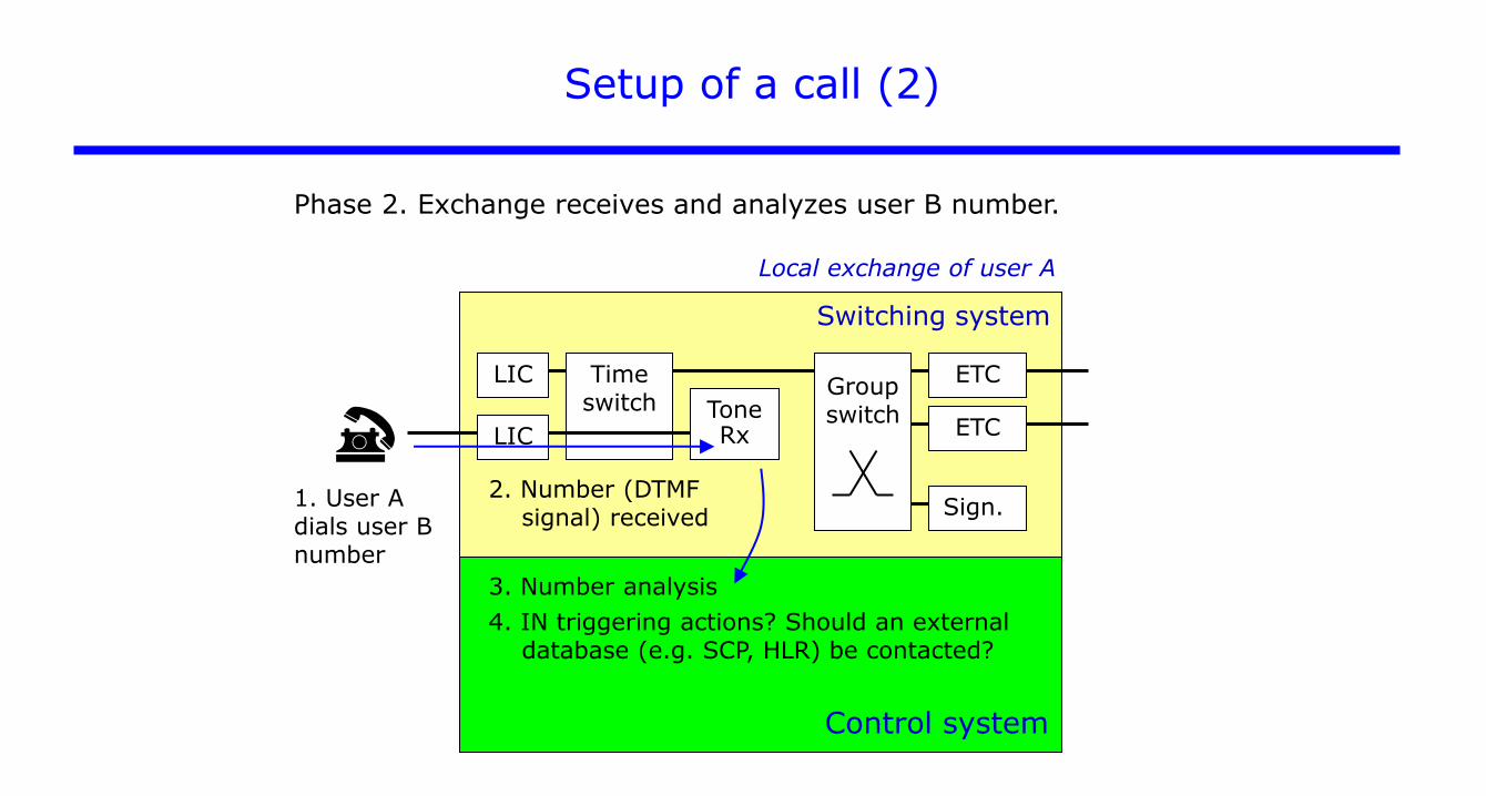
3. Number analysis
Switching system
4. IN triggering actions? Should an external database (e.g. SCP, HLR) be contacted?
LIC
LIC
Tone Rx
Group switch
Sign.
ETC
ETC
Control system
Phase 2. Exchange receives and analyzes user B number.
2. Number (DTMF signal) received
1. User A dials user B number
Setup of a call (2)
Local exchange of user A

Time switch
2. Outgoing circuit is reserved
Switching system
LIC
LIC
Tone Rx
Group switch
Sign.
ETC
ETC
Control system
3. Outgoing signalling message (ISUP IAM) contains user B number
Phase 3. Outgoing circuit is reserved. ISUP Initial address message (IAM) is sent to next exchange.
Setup of a call (3)
1. Tone receiver is disconnected
Local exchange of user A
E.g., CIC = 24
IAM (contains information CIC = 24)

Time switch
1. ISUP ACM message indicates free or busy user B
Switching system
LIC
LIC Group switch
Sign.
ETC
ETC
Control system
3. Charging starts when ISUP ANM message is received
Phase 4. ACM received => ringback or busy tone generated. ANM received => charging starts.
Setup of a call (4)
Local exchange of user A
ACM, ANM Tone generator 2. Ringback
or busy tone is locally generated
4. Call continues…

51
TDM - E1

TDM
• Time division multiplexing allows a link to be utilized simultaneously by many users

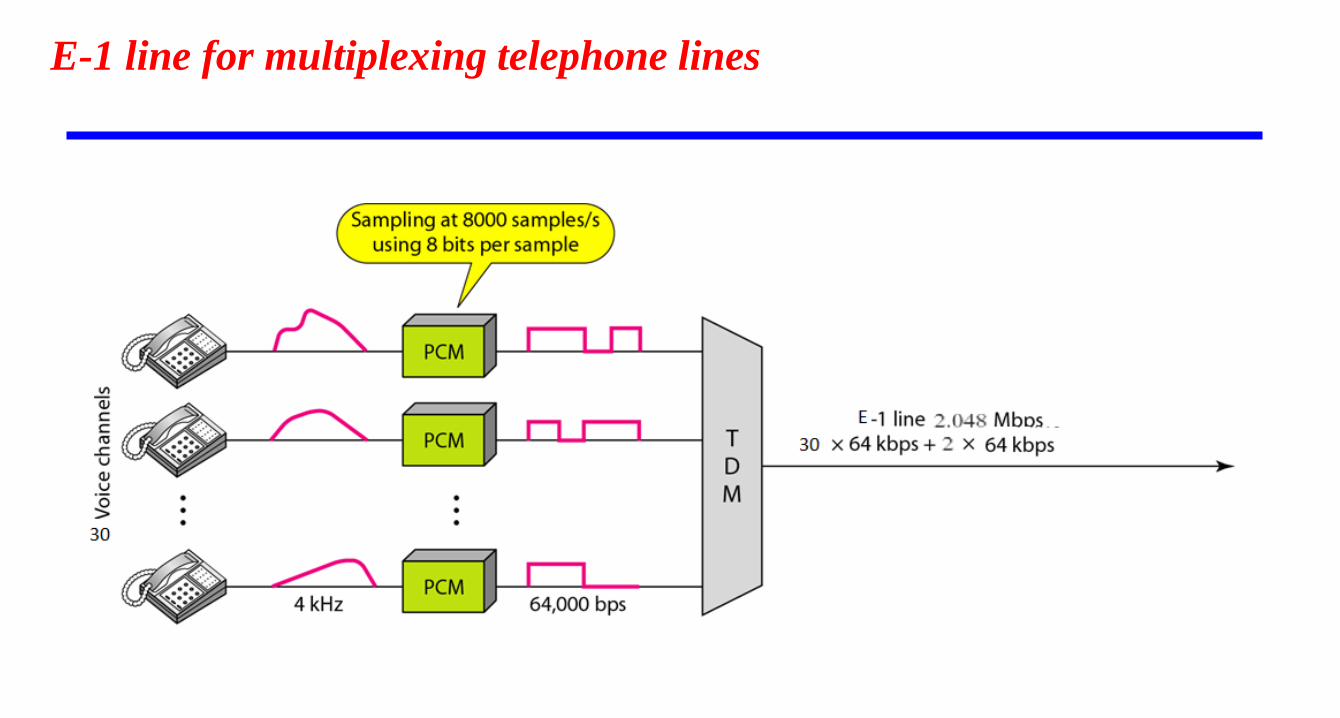
E-1 line for multiplexing telephone lines


TS0-ÇTB Bulma Algoritması
TS: Time Slot – Bir aboneye ait kanal ÇTB: Çerçeve Tanıtım Bilgisi

57
E1 CCS Transmission Format
Applying this framing method to the OMNIBranch and OMNIFlex.
• TS 0 is used for framing and alarm information
• The OMNIBranch assigns channel numbers 1 to 31, for usable transmission.
CCITT G.704 (32 Time Slots)
1 0 2 3 4 5 6 7 8 9 10 11 12 13 14 15 17 16 18 19 20 21 22 23 24 25 26 27 28 29 30 31
OMNIBranch / OMNIFlex - 31 Time Slot Assignments
1 - 2 3 4 5 6 7 8 9 10 11 12 13 14 15 17 16 18 19 20 21 22 23 24 25 26 27 28 29 30 31
Frame (32 Time Slots)
1 0 2 3 4 5 6 7 8 9 10 11 12 13 14 15 17 16 18 19 20 21 22 23 24 25 26 27 28 29 30 31
Speech
Ch. 1-31
Time Slot 0
(8 bits)
0 X 0 1 1 0 1 1 1
0
1
0
1
0
1
0
1
0
1
0
1
0
1
0
Time Slot 1
Speech (Ch. 1)
Frame
Alignment
Word
ITU-T Rec. G.704


Data Traffic Engineering
60

Tele-traffic engineering
• Introduction
• Telephone traffic profile
• Definition
• Trunking
• Congestion
• Traffic performance

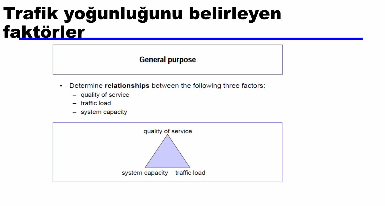
Trafik yoğunluğunu belirleyen faktörler


•In the design of a telecommunication system, initial decision must
be made regarding its size in order to obtain the desired capacity.
•Need to estimate the traffic amount and thus no. of trunks
provided.
•In teletraffic engineering, trunk any entity that will carry one
call. The entity can be international circuit (thousands of km) or
wires in between switches (a few metres).
•The number of trunks to be provided obviously depends on the
traffic to be carried.
•It must be sufficient for the busiest time. However, this will results
in most equipment idling during non-busy hours.
Introduction to Teletraffic Engineering
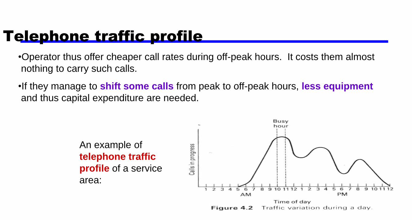
An example of
telephone traffic
profile of a service
area:
•Operator thus offer cheaper call rates during off-peak hours. It costs them almost
nothing to carry such calls.
•If they manage to shift some calls from peak to off-peak hours, less equipment
and thus capital expenditure are needed.
Telephone traffic profile

•It is dimensionless but aThe traffic intensity (sometime referred simply as
traffic) is defined as the average number of calls in progress simultaneously
during a particular period of time.
• Trafik yoğunluğu (bazen trafik olarak da adlandırılır), belirli bir süre boyunca
aynı anda devam eden ortalama çağrı sayısı olarak tanımlanır.
•name has been given to the unit of traffic : Erlang (E) named after A. K. Erlang,
the Danish pioneer in traffic theory.
•One Erlang (E) represents the amount of traffic carried by a trunk that is
completely occupied i.e. one call-hour per hour or one call-minute per minute.
Traffic
Traffic Theory
1915: A. K.
Erlang

•The traffic carried by a
groups of trunks is
T
ChA
A = traffic in Erlangs
C = average number of
call arrivals during
time T
h = average call holding
time
Traffic
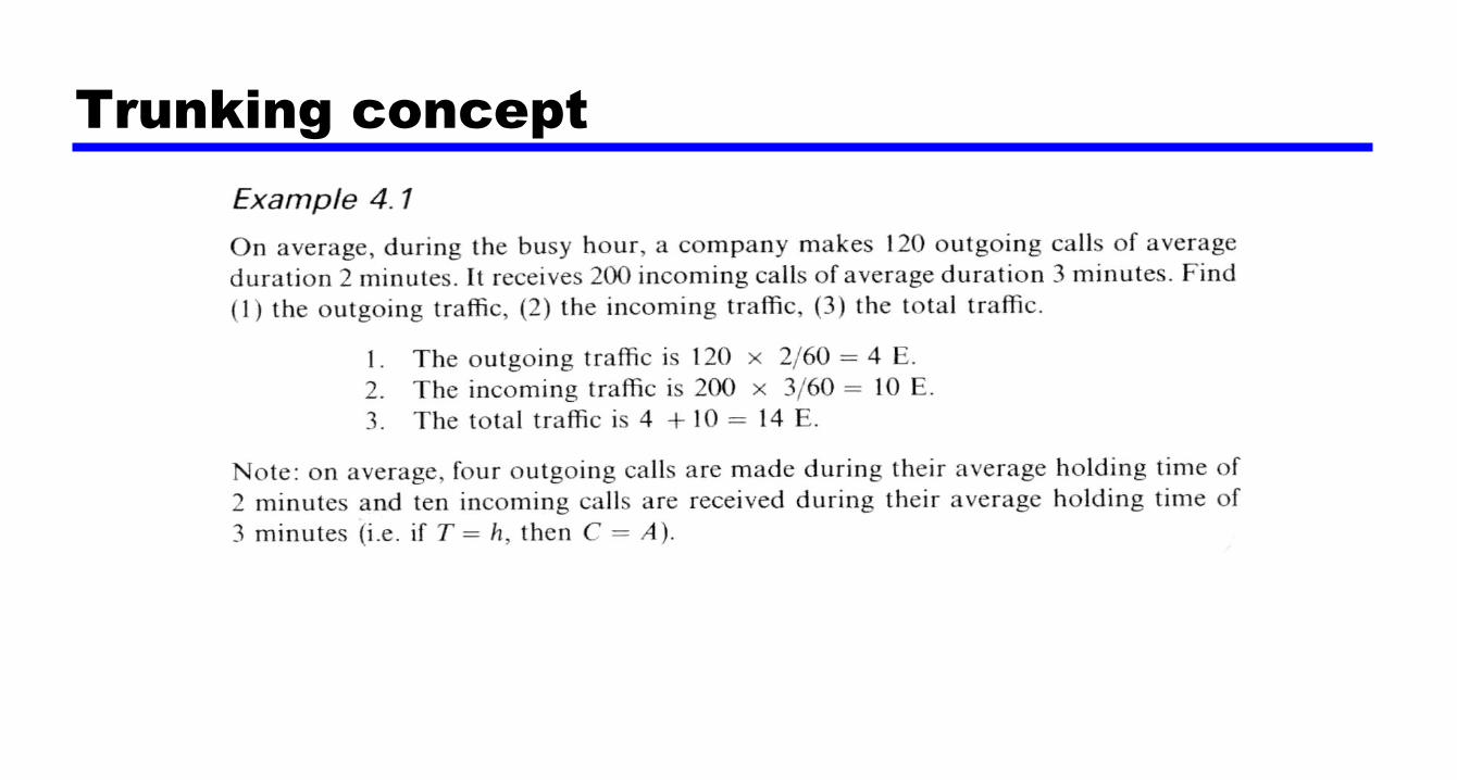
Trunking concept

• The concept of trunking allows a large number of users to
share the relatively small number of trunks/links by
providing access to each user, on demand, from a pool of
available trunks/links.
• Trunking exploits the statistical behaviour of users so that a
fixed number of trunks/links may accommodate a large,
random user community.
• On a group of trunks, the average number of calls in progress
depends on :
1. The number of calls which arrive
2. Their duration (holding time)
Trunking concept

•A single trunk cannot carry more than one call, traffic A for a
single trunk is 1. The traffic is a fraction of an Erlang equal to
the average proportion of time for which the trunk is busy. This is
called the occupancy of the trunk.
•The probability of finding a trunk busy is equal to the proportion of
time for which the trunk is busy. Thus this probability =
occupancy of the trunk.
Trunking concept

• It is uneconomic to provide sufficient equipment to carry all
the traffics that could possibly offered to a telecommunication
system.
• In a telephone exchange, it is possible that all subscribers make
calls simultaneously. The cost of meeting the demand is
prohibitive.
• Therefore, there is a possibility that all trunks in a group of
trunks are busy congestion.
• There are 2 types of telecommunication system :
1. Lost Call (LC) system
2. Delay/queuing system
Congestion
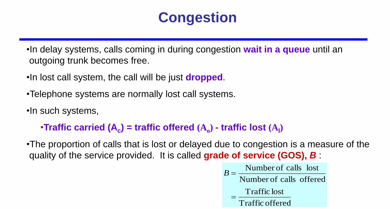
•In delay systems, calls coming in during congestion wait in a queue until an
outgoing trunk becomes free.
•In lost call system, the call will be just dropped.
•Telephone systems are normally lost call systems.
•In such systems,
•Traffic carried (Ac) = traffic offered (Ao) - traffic lost (Al)
•The proportion of calls that is lost or delayed due to congestion is a measure of the
quality of the service provided. It is called grade of service (GOS), B :
offered Traffic
lost Traffic
offered calls ofNumber
lost calls ofNumber
B
Congestion

B = proportion of the time for which congestion exists.
= probability of congestion.
= probability that a call will be lost due to congestion.
•Thus, if traffic Ao Erlangs is offered to a group of trunks having a GOS, B, the traffic lost is AoB and the traffic carried is
• Ac = Ao(1 - B)
•The larger the GOS, the worse is the service given.
•If GOS is too large it will results in many users unable to make successful calls and thus dissatisfied.
•If GOS is too small, unnecessary expenditure on equipment which is rarely used is made.
•In practice, GOS is higher for more expensive trunks.
Congestion
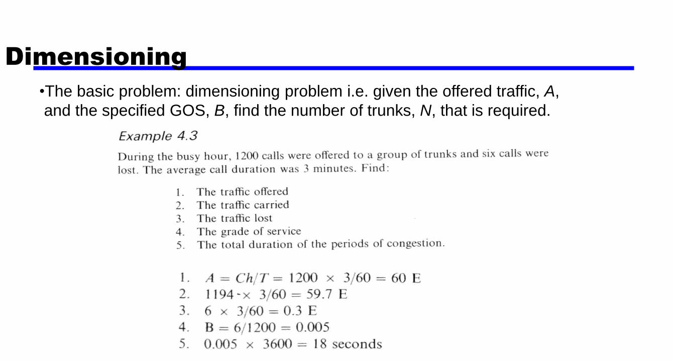
•The basic problem: dimensioning problem i.e. given the offered traffic, A,
and the specified GOS, B, find the number of trunks, N, that is required.
Dimensioning

•In order to obtain analytical solutions to teletraffic problems, it is necessary to have a
mathematical model of the traffic offered.
•A simple model is based on the following assumptions :
(1) Pure-chance traffic - call arrivals and terminations are independent random
events.
(2) Statistical equilibrium - the generation of traffic is a stationary random process
i.e. the probabilities do not change during the period considered.
Traffic model

•The number of call arrival in a given period of time, T has Poisson distribution.
•The intervals between call arrivals, T are intervals between two independent events and the distribution is given
by a negative exponential distribution
•The call duration, H is modelled as a negative exponential distribution
•For a group of N trunks the number of calls in progress varies randomly. This is an example of birth and death
process or renewal process.
•The number of calls in progress (i.e., so called the state) is always between 0 and N.
•Such process is called a simple Markov chain. Its behaviour depends on the probability of change from each state
to one state before or after the state.
Traffic model
ex
xPx
!

•Simple Markov chain.
State probabilities
Transition probabilities
•At statistical equilibrium, the probabilities do not change and
process becomes regular Markov chain.
Traffic model
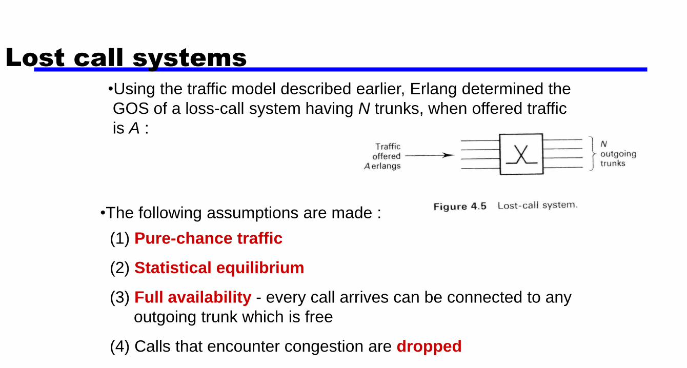
•Using the traffic model described earlier, Erlang determined the
GOS of a loss-call system having N trunks, when offered traffic
is A :
Lost call systems
•The following assumptions are made :
(1) Pure-chance traffic
(2) Statistical equilibrium
(3) Full availability - every call arrives can be connected to any
outgoing trunk which is free
(4) Calls that encounter congestion are dropped
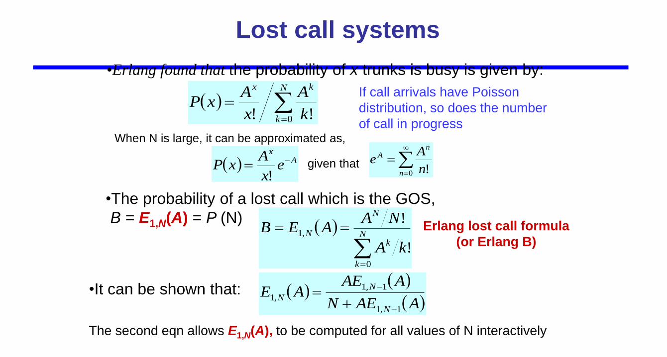
•The probability of a lost call which is the GOS,
B = E1,N(A) = P (N)
N
k
k
N
N
kA
NAAEB
0
,1
!
!Erlang lost call formula
(or Erlang B)
Lost call systems
•Erlang found that the probability of x trunks is busy is given by:
Ax
ex
AxP
!
0 !n
nA
n
Aegiven that
When N is large, it can be approximated as,
If call arrivals have Poisson
distribution, so does the number
of call in progress
N
k
kx
k
A
x
AxP
0 !!
•It can be shown that:
AAEN
AAEAE
N
N
N
1,1
1,1
,1
The second eqn allows E1,N(A), to be computed for all values of N interactively

A group of five trunks is offered 2E of traffic. Find:
1. The grade of service
2. The probability that only one trunk is busy
3. The probability that only one trunk is free
4. The probability that at least one trunk is free
Solutions:
1. From Erlang lost call
formula
Lost call systems
2. From
N
k
kx
k
A
x
AxP
0 !!
P(1) = 2/7.2667 = 0.275
3) P(4) = (16/24)/7.2667 = 0.0917
4. P(x<5) = 1 – P(5)
= 1 – B = 1 – 0.037 = 0.963

Lost call systems

•If the offered traffic, A increases, the number of trunks, N, must obviously be increased
to provide a given GOS.
•However, for the same trunk occupancy (or utilization), the probability of finding all
trunks busy is less for a large group of trunks than for a small group.
•Thus for a given GOS, trunk occupancy is higher in a large group of trunks than a
small group large group is more efficient.
•This is the concept of trunking as explained earlier or principle of concentration: it is
more efficient to concentrate traffic onto a single large group of trunks.
Traffic performance

•Example : for trunk groups dimensioned to provide GOS of 0.002
at their normal load, a 5-trunk group suffers GOS increase of 40%
when traffic overload of 10% occurs while a 100-trunk group
suffers a 550% increase in GOS.
•Most telecommunications operators adopt dual criteria: two
GOSs are specified - one at normal traffic load and another,
larger GOS for a given percentage of overload.
•The number of trunks provided is determined by which criterion
requires the greater number.
Traffic performance

Traffic performance

•Connection between users may span over multiple links in the
system.
•Thus the GOS for the whole connection needs to be determined.
•Lets look at example of two links connection with each link
having GOS, B1 and B2.
Traffic offered to second link = A(1 - B1)
Traffic reaching destination = A(1 - B1)(1 - B2)
= A(1 + B1 B2 - B1 - B2)
Loss systems in tandem

The overall GOS = B1 + B2 - B1 B2.
If B1, B2 << 1, then B1 B2 is negligible and the overall GOS is B1 +
B2.
•In general, for an n-link connection, the GOS is
n
k
kBB1
Loss systems in tandem

•E1,N(A) is suitable for solving problems : given A and N, find B.
•However, in network dimensioning the problem is : given A and
B, find N. The equation given earlier is not suitable. Calculated
values in table can be used..
(next page)
(slide 22)
Traffic tables

91
Traffic Engineering (E1)
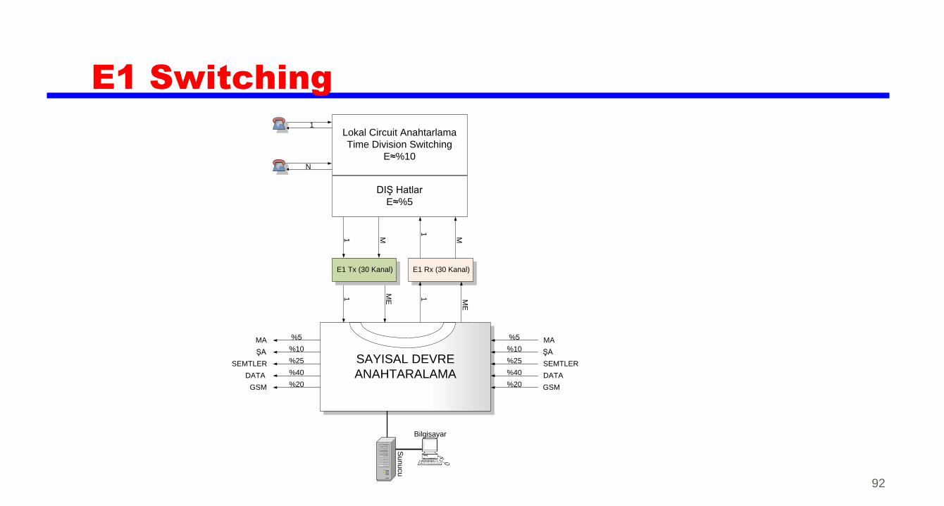
E1 Switching
92
Lokal Circuit Anahtarlama
Time Division Switching
E≈%10
1
N
1 M
1 ME
1
SAYISAL DEVRE
ANAHTARALAMA
%5 MA
1
M
E1 Tx (30 Kanal) E1 Rx (30 Kanal)
ME
%10 ŞA
%25 SEMTLER
%40 DATA
%20 GSM
%5MA
%10ŞA
%25SEMTLER
%40DATA
%20GSM
Su
nu
cu
Bilgisayar
DIŞ Hatlar
E≈%5

Örnek: Abone sayısı 12000; İç Trunk Earlang=%10; Dış Trunk
Earlang=%20; Şae=%10, Mae=%5, See=%25, Dae=%40, GSMe=%20
• N=12000, ITE=%10, DTE=%20
• Niç=NxITE=12000 x 10 /100=1200 Abone, Aynı anda; maksimum alet (devre ya da sistem)
• Ndış=Niç x DTE = 1200 x 20 /100=240 Abone (PCM, 64Kbps)
• Hesap edilen Dış anahtarlama E1 sayısı=240/30=8 E1
• ŞAE1=8 x 10/100=0.8E1; Toplam Kanal sayısı=0.8 x 30 =24KK; ŞAE1=1 E1 alınır.
• MAE1=8 x 5/100=0.4E1; Toplam Kanal sayısı=0.4 x 30 =12KK; ŞAE1=1 E1 alınır.
• SemtE1=8 x 25/100=2E1; Toplam Kanal sayısı=2 x 30 =60KK; ŞAE1=2 E1 alınır.
• DataE1=8 x 40/100=3.2E1; Toplam Kanal sayısı=3.2 x 30 =96KK; ŞAE1=4 E1 alınır. (Kanal Planlama: 30 + 30 + 30 + 6)
• GSME1=8 x 20/100=1.6E1;Toplam Kanal sayısı=1.6 x 30 =48KK; ŞAE1=2 E1 alınır.
(Kanal: 30 + 18)
• >Planlanan E1=10 E1
93

94
DSM
E1
E10
E1 Rx
Tx
Rx Tx E10
Digital Switching Matrix & E1 Switching

E1- TDM: Time Slot Switching – DSM (Digital
Switching Matrix)

DSM
E1
E25
1
25
Rx Tx
Rx Tx
E16
Rx
E21
Rx
E16 Tx
E21 Tx
CH
5
CH
5
CH
20
CH
20
Örnek: Toplam E1 sayısı 25 olan DSM de 455 nolu
aboneyi 620 nolu aboneye anahtarlayın
• A) Toplam abone sayısı=25 x 30 =750
• B) 455 nolu ve 620 nolu aboneler kanalı hangi E1 de?
455/30=15. …; 16 nolu E1’in 5 nolu kanalı
620/30=20. …; 21 nolu E1’in 20 nolu kanalı
• C) Anahtarlama

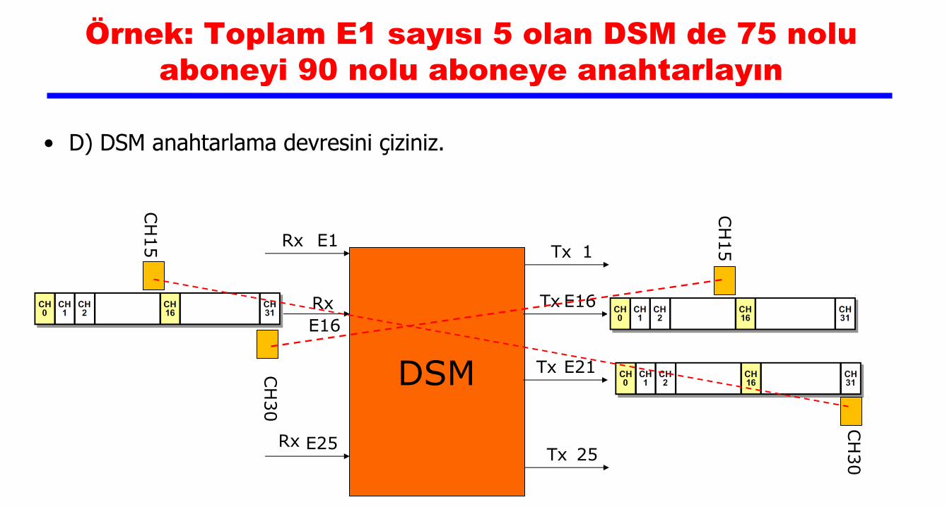
Örnek: Toplam E1 sayısı 5 olan DSM de 75 nolu
aboneyi 90 nolu aboneye anahtarlayın
• A) Toplam aynı anda hizmet alacak abone sayısı=5 x 30 =150
• B) Kanal Sıralaması yapınız
1. E1 Kanal Sıralama: 1…30
– 2. E1 Kanal Sıralama: 31…60
– 3. E1 Kanal Sıralama : 61… 90
– 4. E1 Kanal Sıralama : 91 … 120
– 5. E1 Kanal Sıralama : 121 … 150
• C) Anahtarlanacak abonelerin konumlarını belirleyin
• 75 nolu abone: 3. E1’in 15 nolu kanalı
• 90 nolu abone: 3.E1’in 31 nolu kanalı(0: ÇTB, 16: ÇÇTB ve Sinyalleşme, Abone kanalları: 1..15, 17..31)
DSM
E1
E25
1
25
Rx Tx
Rx Tx
E16
Rx E16 Tx
E21 Tx
CH
15
CH
15
CH
30
CH
30
Örnek: Toplam E1 sayısı 5 olan DSM de 75 nolu
aboneyi 90 nolu aboneye anahtarlayın
• D) DSM anahtarlama devresini çiziniz.

Örnek: Toplam E1 sayısı 8 olan DSM de 6. E1 10. Kanalı 4.E1 in 29. Kanalına
anahtarlanmıştır. DSM anahtarlama devresini çiziniz. Abone numaralarını bulunuz
• A) Abone numaralarını bulunuz.
• Aynı anda hizmet alacak toplam abone sayısı: 8 x 30=240
• Kanal Sıralaması:
1. E1 Kanal Sıralama: 1…30
– 2. E1 Kanal Sıralama: 31…60
– 3. E1 Kanal Sıralama : 61… 90
– 4. E1 Kanal Sıralama : 91 … 120
– 5. E1 Kanal Sıralama : 121 … 150
– 6. E1 Kanal Sıralaması: 151 … 180
– 7. E1 Kanal Sıralaması: 181 … 210
– 8. E1 Kanal Sıralaması: 211 … 240
• 6. E1 10.Kanal: 5 x 30 + 10=150 +10=160
• 4. E1 29. Kanal: 3 x 30 +30 =120 (ÇÇTB: 16. Kanal)

100
Traffic Engineering (PSTN- CODEC)

Incoming PCM Junction Switching
101
Lokal Circuit Anahtarlama
Time Division Switching
E≈%10
1
N
1 M
1 ME
1
SAYISAL DEVRE
ANAHTARALAMA
%5 MA
1
M
E1 Tx (30 Kanal) E1 Rx (30 Kanal)
ME
%10 ŞA
%25 SEMTLER
%40 DATA
%20 GSM
%5MA
%10ŞA
%25SEMTLER
%40DATA
%20GSM
Su
nu
cu
Bilgisayar
DIŞ Hatlar
E≈%5

Örnek: Abone sayısı 12000; İç Trunk Earlang=%10; Dış Trunk
Earlang=%20; 30 Kanal 1 E1 olduğuna göre E1 sayısını bulunuz.
• N=12000, ITE=%10, DTE=%20
• Niç=NxITE=12000 x 10 /100=1200 Abone, Aynı anda; maksimum alet (devre ya da sistem)
• Ndış=Niç x DTE = 1200 x 20 /100=240 Abone (PCM, 64Kbps)
• Dış anahtarlama E1 sayısı=240/30=8 E1
102
DSM
E1
E8
E1 Rx Tx
Rx Tx E8

Incoming GSM Switching
103
1
N
1 M
1 ME
1
SAYISAL DEVRE ANAHTARALAMA
%5 MA
1 M
E1 Tx (30
Kanal)E1 Rx (30 Kanal)
ME
%10 ŞA%25 SEMTLER%40 DATA%20 GSM
%5MA%10ŞA%25SEMTLER%40DATA%20GSM
Su
nu
cu
Bilgisayar
DIŞ Hatlar
E≈%10
Boş Kanal Bulma
E≈%20

Kaynaklar
• Analog Electronics, Bilkent Unıversity • Electric Circuits Ninth Edition, James W. Nilsson Professor Emeritus Iowa State University,
Susan A. Riedel Marquette University, Prentice Hall, 2008. • Lessons in Electric Circuits, By Tony R. Kuphaldt Fifth Edition, last update January 10, 2004. • Fundamentals of Electrical Engineering, Don H. Johnson, Connexions, Rice University,
Houston, Texas, 2016. • Introduction to Electrical and Computer Engineering, Christopher Batten - Computer
Systems Laboratory School of Electrical and Computer Engineering, Cornell University, ENGRG 1060 Explorations in Engineering Seminar, Summer 2012.
• Introduction to Electrical Engineering, Mulukutla S. Sarma, Oxford University Press, 2001. • Basics of Electrical Electronics and Communication Engineering, K. A. NAVAS Asst.Professor
in ECE, T. A. Suhail Lecturer in ECE, Rajath Publishers, 2010. • http://www.ee.cityu.edu.hk/~csl/sigana/sig01.ppt • İnternet ortamından sunum ve ders notları
104

Usage Notes
• These slides were gathered from the presentations published on the internet. I would like to thank who prepared slides and documents.
• Also, these slides are made publicly available on the web for anyone to use
• If you choose to use them, I ask that you alert me of any mistakes which were made and allow me the option of incorporating such changes (with an acknowledgment) in my set of slides.
Sincerely,
Dr. Cahit Karakuş
105

106


