Chapter 3 Ethics economics and the environment 3.1 Naturalist moral philosophies 3.2 Libertarian moral philosophy 3.3 Utilitarianism 3.4 Criticisms of utilitarianism 3.5 Intertemporal distribution And God said, Let us make man in our image, after our likeness: and let them have dominion over the fish of the sea, and over the fowl of the air, and over the cattle, and over all the earth, and over every creeping thing that creepeth upon the earth. Verse 26, Book of Genesis, The Bible, King James Translation. Some claim ‘dominion over’ would be better translated as ‘stewardship of’
Transcript
Chapter 3 Ethics economics and the environment
3.1 Naturalist moral philosophies
3.2 Libertarian moral philosophy
3.3 Utilitarianism
3.4 Criticisms of utilitarianism
3.5 Intertemporal distribution
And God said, Let us make man in our image, after our likeness: and let them have dominion over the fish of the sea, and over the fowl of the air, and over the cattle, and over all the earth, and over every creeping thing that creepeth upon the earth. Verse 26, Book of Genesis, The Bible, King James Translation.
Some claim ‘dominion over’ would be better translated as ‘stewardship of’
Why consider ethics?
The question ‘What will happen to petrol consumption if the tax on it is increased by x%?’ is a question for positive economics. It does not entail any ethical considerations.
The question ‘Should the tax on petrol be increased?’ is a question for normative, or welfare, economics. It can only be answered using ethical criteria.
Much of environmental and resource economics is about questions of the ‘should’ type – questions about the targets and instruments of policy.
The ethical criteria that welfare economics uses are Utilitarian. To understand the basis for the welfare economics that environmental and resource economics draws on, it is necessary to consider the Utilitarian ethical system that underlies welfare economics.
There are other ethical systems.
Naturalist moral philosophies
Naturalist ethical systems treat non-human entities as morally considerable.
Deep ecology is a naturalist ethic.
‘A thing is right when it tends to preserve the integrity, stability and beauty of the biotic community. It is wrong otherwise.’ from A Sand County Almanac by Aldo Leopold
There are two broad classes of ethical system:
1.Consequentialist systems judge actions by the consequences that follow from them
2.Deontological systems judge actions by whether they fulfil obligations
One can arrive at a naturalist position from either of these systems:
1.By extending beyond humans the entities for whom consequences count (Singer 1993)
2.By extending beyond humans the entities to whom obligations are owed (Watson 1979)
Libertarian moral philosophy
Libertarianism is a humanist ethical system. Its basic axiom is that individual human rights are inviolable. Rights attach only to individual humans. Any infringement of such cannot be justified by the consequences arising.
Libertarianism implies a very limited role for government. For many libertarians government action would basically be limited to maintaining the institutions required to support free contracting and exchange.
Income and wealth redistribution from rich to poor should happen only to the extent that everybody agrees to, otherwise it is coercive and unjust.
The best known modern Libertarian philosopher is Nozick (1974)
Utilitarianism
Utilitarianism is a consequentialist moral philosophy. It is the consequences of an action that determine its moral worth. The ends may justify the means, as with a lie that saves a life.
The application of utilitarianism requires the definition of the set of entities for whom consequences are to be considered. Usually the set is restricted to humans. But Singer (1993) for example argues that it should include all sentinent beings capable of pleasure and pain.
The utilitarianism that underpins welfare economics is anthropocentric – the set of morally considerable entities is restricted to humans. But, consequences for non-human entities will enter in so far as humans are affected by them.
Often in economics, the set of humans considered is the citizens of a nation state.
In economics, what is good/bad for a human individual (increases/decreases utility) is self-assessed, determined by that individual’s preferences. This is preference satisfaction utilitarianism. Consumer sovereignty follows – economic outcomes should reflect consumer preferences.
Social welfare is some aggregation of individuals’ utilities.
Cardinal and ordinal utility functions
For an individual a utility function maps states of the world into a single number for utility
U = U(X1, X2,....Xi,...XN)
Aggregation over individuals requires that U’s are cardinal numbers (weight, height, distance). The standard operations of arithmetic do not apply for ordinal numbers, which indicate only ranking ( street numbers). Cardinality makes interpersonal comparison possible.
The standard propositions of demand theory can be derived from ordinal utility functions, and many economists are reluctant to assume cardinality and admit interpersonal comparisons.
In which case, policy advice is restricted to the application of compensation tests ( to be discussed in Chapter 4) which ignore distributional issues. Much of applied welfare economics, as in environmental economics, does ignore distribution ( fairness/equity/justice) and focus on efficiency via compensation tests.
If cardinality is assumed, aggregation can use a social welfare function.
The social welfare function Max W = W(UA, UB)
Subject to UA = UA(XA) and UB = UB(XB)
and X = XA + XB
gives the necessary condition
WAUAX = WBUB
X
where WA and WB are the derivatives of the social welfare function wrt UA and UB and UA
X and UBX are the derivatives of the utility functions, marginal utilities, so that
the condition is that marginal contributions to social welfare from each individual’s consumption are equal.
For W = wAUA(XA) + wBUB(XB)
where wA and wB are fixed weights the condition is
wAUAX = wBUB
X
and for wA = wB = 1 so that the fixed weights are equal
UAX = UB
X
In this case, if the individuals have the same utility functions, social welfare maximisation implies equal consumption levels.
Social welfare maximisation – a special case
Figure 3.2 Maximisation of social welfare subject to a constraint on the total quantity of goods available
Figure 3.1 shows one indifference curve, drawn in utility space, for W = UA + UB. Figure 3.2 is drawn in consumption space, where, assuming diminishing marginal utility, the welfare indifference curves are convex from below. Maximisation of welfare subject to the constraint of a fixed amount available gives equal consumption for the two individuals.
This is a special case.
Social welfare maximisation with different utility functions
Equal consumption levels for welfare maximisation is not the general case. It is not the result if
1.the SWF is linear with unequal weights and the U functions are the same
or
2. the SWF is linear with equal weights and the U functions differ
In Figure 3.3 A gets more utility than B for the same level of consumption. The marginal utilities are equal at different levels of consumption.
Individual A is more ‘efficient’ at turning consumption into utility – is a better ‘pleasure machine’ – and so welfare maximisation with equal weights assigns her more consumption.
Is this ‘fair’?
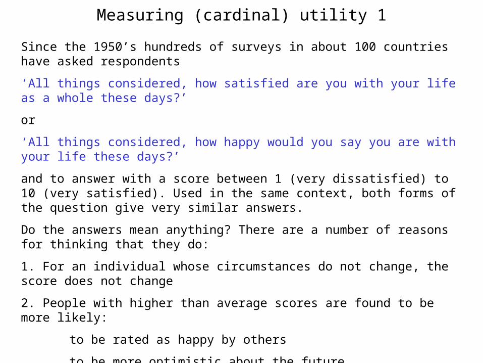
Measuring (cardinal) utility 1
Since the 1950’s hundreds of surveys in about 100 countries have asked respondents
‘All things considered, how satisfied are you with your life as a whole these days?’
or
‘All things considered, how happy would you say you are with your life these days?’
and to answer with a score between 1 (very dissatisfied) to 10 (very satisfied). Used in the same context, both forms of the question give very similar answers.
Do the answers mean anything? There are a number of reasons for thinking that they do:
1. For an individual whose circumstances do not change, the score does not change
2. People with higher than average scores are found to be more likely:
to be rated as happy by others
to be more optimistic about the future
to be less likely to attempt suicide
to smile more in social interaction
to recall more positive than negative life events
to be healthier
Measuring (cardinal) utility 2 3. Both questions have been used in the same circumstances giving almost identical rankings across country averages
4. Across individuals responding to a given survey, individual scores are found to correlate with attributes in plausible ways that are generally replicated across surveys. The following correlate positively:
absolute income
income relative to others
income relative to past income
being married
being a member of a group ( eg religious )
political participation
good physical health
The following correlate negatively:
Unemployment
Job insecurity
Direction of causation? Tracking the same respondents over time suggests that it runs from circumstances to happiness score.
Happiness and income1.Looking at country average scores at a point in time, most studies find diminishing marginal utility, as in Figure 3.4
2.Looking at individuals in a given country at a point in time, most studies find diminishing marginal utility. The evidence for this is less strong in developing countries
3. Looking at one country over time, which has been done only for some developed countries, it is found that the national average score is weakly related to GDP pc. In Figure 3.5 for the USA, GDP pc increased steadily while the % reporting themselves very happy actually fell slightly over 1946-1996.
A paradox Proportion of
peoplewith incomes
in the top quarter ofthe range
%
Proportion of people
with incomesin the bottom
quarterof the range
%State reported
1975 1998 1975 1998
Very happy 39 37 19 16
Pretty happy
53 57 51 53
Not too happy
8 6 30 31
Table 3.1 Percentages reporting various states of happiness by income group, USA
Looking across individuals and countries at a point in time, income and happiness are positively related. albeit with declining marginal utility.
BUT if we look at a rich economy over time, rising GDP per capita does not go with increasing self-assessed happiness/satisfaction.
Table 3.1 illustrates.
The resolution of the paradox widely agreed in the happiness literature is in
terms of Adaptation, Aspiration and Interdependencies
Resolving the paradox
1.An individual’s utility depends on the relationship between her outcomes and her aspirations, and on the relationship between her outcomes and those of others. For individual 1 at time t
where A for aspiration and E for experience = outcome in j=1,2...m areas, O denotes others.
2. An individual’s aspirations depend on her own past experiences
A1jt = h1j(E1jt-1, E1jt-2,.......E1jt-T)
Then, a rise in 1’s income means increased consumption of 1, which is, say, clothes – higher E11 for given A11 and EO1 means higher U1 initially. But she gets used to her new clothes and A11 adjusts to past E11, reducing U1. The novelty wears off - adaptation.
In a growing economy, the consumption of others is rising along with that of 1, working to restore the gap between E11 and E01, and to reduce U1 back toward its former level. This is interdependence as rivalry.
Adaptation and rivalry are everyday experience, but not much taken account of in economics to date, where the standard utility function is:
U1t = U1(E11t,E12t,....E1jt,....E1mt)
ImplicationsThe results of ‘happiness research’ clearly have implications for both positive and normative, ie welfare, economics, and hence for environmental and resource economics.
Welfare economics recognises interpersonal interdependencies, as person to person externalities (chapter 4), but relates them to material interdependencies, and treats them as exceptional.
Results from happiness research suggest that interpersonal interdependencies can be purely psychological, and are not in the least exceptional.
Layard (2005a and 2005b) considers the implications for thinking about income taxation. According to standard public economics, income taxation is regrettable necessity (because lump sum taxation is not feasible) which distorts the choice between consumption and leisure. It should be kept as low as possible.
Layard points out that this result depends on the assumption that there are no externalities involved in the work (to consume)/leisure choice, whereas happiness research shows that there are. Each individual’s choice is affected by that of others. Given that, income taxation can be seen as an externality correcting policy, rather than a distortion, akin to a tax on pollution.
What the results of happiness research imply for the policy prescriptions of environmental and resource economics has yet to be worked out.
Criticism of preference based utilitarianism
The kind of utilitarianism that welfare economics is based on has it that individuals are the best judge of what is good/bad for them, so that individuals’ preferences tell the analyst what is good for individuals.
Two lines of criticism of this particular version of utilitarianism can be distinguished:
1.Taking preferences as given and truly reflecting interests, is it reasonable to assume that individuals generally have enough information to assess the implications for their utility of the alternatives open to them?
2. Is it reasonable to assume that, in a world where socialisation processes and advertising are pervasive, peoples’ preferences do truly reflect their interests?
Sen (1987) has argued that people are dualistic, being concerned with the satisfaction of their own preferences and pursuing objectives which are not exclusively self-interested. Sen distinguishes between altruism as ‘sympathy’ and ‘commitment’. Sympathy is where my concern is reflected in arguments in my utility function, so that if a change improves the lot of relevant other(s), my utility increases. Commitment is where my concern is based on my ethical principles, which may lead me to approve of change that reduces my utility. Individuals exist as both consumers and citizens.
Rawls: A Theory of Justice
Rawls objects to classical utilitarianism on the grounds that simply maximising the sum of individual utilities, and ignoring their distribution, could lead to outcomes that violate fundamental rights.
Rawls looks to establish the principles of a just society by asking what would be agreed by everyone if we could freely, rationally and impartially consider just arrangements. To do this, he uses the ‘original position’, in which individuals exist behind a ‘veil of ignorance’ – no person has knowledge of what their circumstances would be in the world for which they are deliberating the nature of a ‘social contract’.
Rawls claims that there would be unanimous agreement on two fundamental principles of justice
Each person to have a right to the most extensive liberty compatible with the same for others
Social and economic inequalities to be arranged so that they are (a) expected to be to everyone’s advantage and (b) attached to positions and offices open to all
The second of these is the Difference Principle. It asserts that inequalities are justified only if they enhance everyone’s position – if they lead to Pareto improvements. There is a presumption in favour of equality.
Rawlsian utilitarianism 1
One way to give utilitarianism a Rawlsian character is to use a particular form of Social Welfare Function, which for two individuals would be
W = min(UA, UB) (3.8)
so that W is the smallest of UA and UB.
Raising utility for the worst off will increase welfare. Re-allocating db from B to A, de = db, gives e.
The 45o line, UA = UB, gives maximum levels of welfare.
Rawlsian utilitarianism 2(a)
Iso-elastic Utility Functions
1ηand0ηforη1
XU
η1
(3.9)
U = lnX for η = 1 (3.10)
η is the elasticity of marginal utility with respect to consumption X
η1
X
η1
XW
η1Bη1A
(3.11)
W = lnXA + lnXB (3.12)
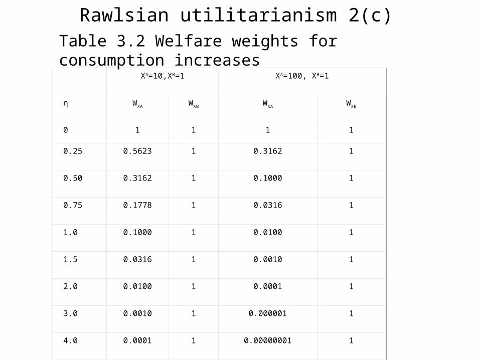
Rawlsian utilitarianism 2(b)
For η = 0, the SWF on iso-elastic U functions treats an extra unit of consumption equally across individuals
For η = ,1 it treats equal proportional increases in consumption equally across individuals
For η > 1, it treats an x% increase for the poorer person as more welfare increasing than x% for the better-off person.
As η goes to infinity, so small U increases for the worst-off get weighted much more than large U increases for the better-off. In the limit, increases in U for the better-off have no effect on welfare.
Rawlsian utilitarianism 2(c)
XA=10,XB=1 XA=100, XB=1
η WXA WXB WXA WXB
0 1 1 1 1
0.25 0.5623 1 0.3162 1
0.50 0.3162 1 0.1000 1
0.75 0.1778 1 0.0316 1
1.0 0.1000 1 0.0100 1
1.5 0.0316 1 0.0010 1
2.0 0.0100 1 0.0001 1
3.0 0.0010 1 0.000001 1
4.0 0.0001 1 0.00000001 1
Table 3.2 Welfare weights for consumption increases
Intertemporal distribution 1Simplifying assumptions
Constant population size
Consider the ‘representative individual’ alive at each point in time
The utility function is invariant over time
Then work with a SWF that aggregates utilities at different dates – so assuming cardinally measurable utility
Generally, for two years
W = W(U0, U1)
and usually for utilitarianism
W = φ0U0 + φ1U1 (3.13)
with φ0 = 1 and φ1 = 1/(1+ρ)
so that
W = U0 + U1/(1+ ρ) (3.14)
where ρ is the utility discount rate
Intertemporal distribution 2
tt
T=t
0=ttt
T=t
0=t
TT1100
UU)ρ+(1
1=
U)ρ+(1
1 +...+ U
)ρ+(1
1 + U
)ρ+(1
1 =W
t
t ρ)(1
tt
=t
0=t
tt
=t
0=t
UU)ρ+(1
1 =W
dtU =dte U=W t
t
0t
tρt
t
=t
0=t
ρt
t e
(3.15)
where
For an infinite time horizon
(3.16)
In continuous time
(3.17)
where
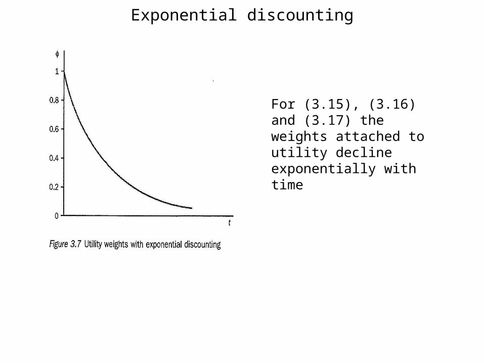
Exponential discounting
For (3.15), (3.16) and (3.17) the weights attached to utility decline exponentially with time
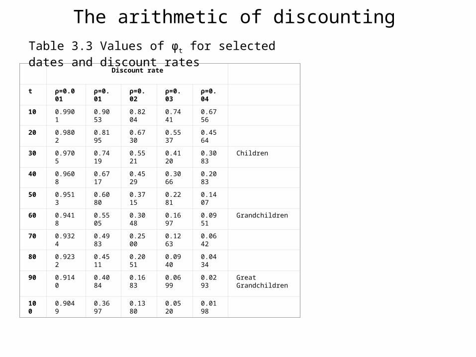
The arithmetic of discounting
Discount rate
t ρ=0.001
ρ=0.01
ρ=0.02
ρ=0.03
ρ=0.04
10 0.9901
0.9053
0.8204
0.7441
0.6756
20 0.9802
0.8195
0.6730
0.5537
0.4564
30 0.9705
0.7419
0.5521
0.4120
0.3083
Children
40 0.9608
0.6717
0.4529
0.3066
0.2083
50 0.9513
0.6080
0.3715
0.2281
0.1407
60 0.9418
0.5505
0.3048
0.1697
0.0951
Grandchildren
70 0.9324
0.4983
0.2500
0.1263
0.0642
80 0.9232
0.4511
0.2051
0.0940
0.0434
90 0.9140
0.4084
0.1683
0.0699
0.0293
Great Grandchildren
100
0.9049
0.3697
0.1380
0.0520
0.0198
Table 3.3 Values of φt for selected dates and discount rates
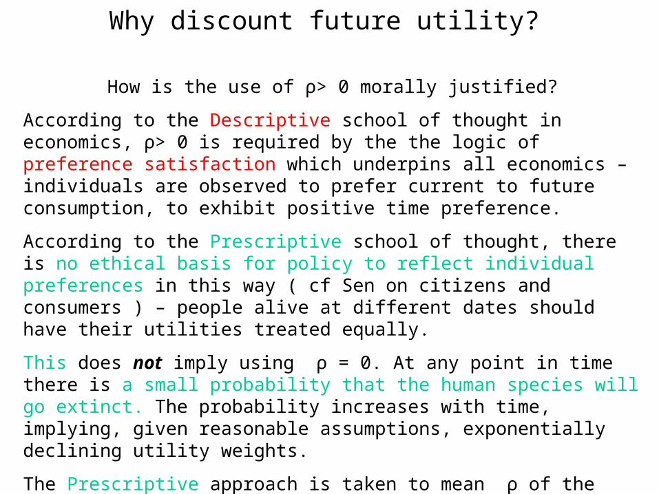
Why discount future utility?
How is the use of ρ> 0 morally justified?
According to the Descriptive school of thought in economics, ρ> 0 is required by the the logic of preference satisfaction which underpins all economics – individuals are observed to prefer current to future consumption, to exhibit positive time preference.
According to the Prescriptive school of thought, there is no ethical basis for policy to reflect individual preferences in this way ( cf Sen on citizens and consumers ) – people alive at different dates should have their utilities treated equally.
This does not imply using ρ = 0. At any point in time there is a small probability that the human species will go extinct. The probability increases with time, implying, given reasonable assumptions, exponentially declining utility weights.
The Prescriptive approach is taken to mean ρ of the order of 0.001, 0.1%.
The Descriptive approach is taken to mean ρ of the order of 0.03, 3%.
The difference matters a lot – more in Chapter 11.
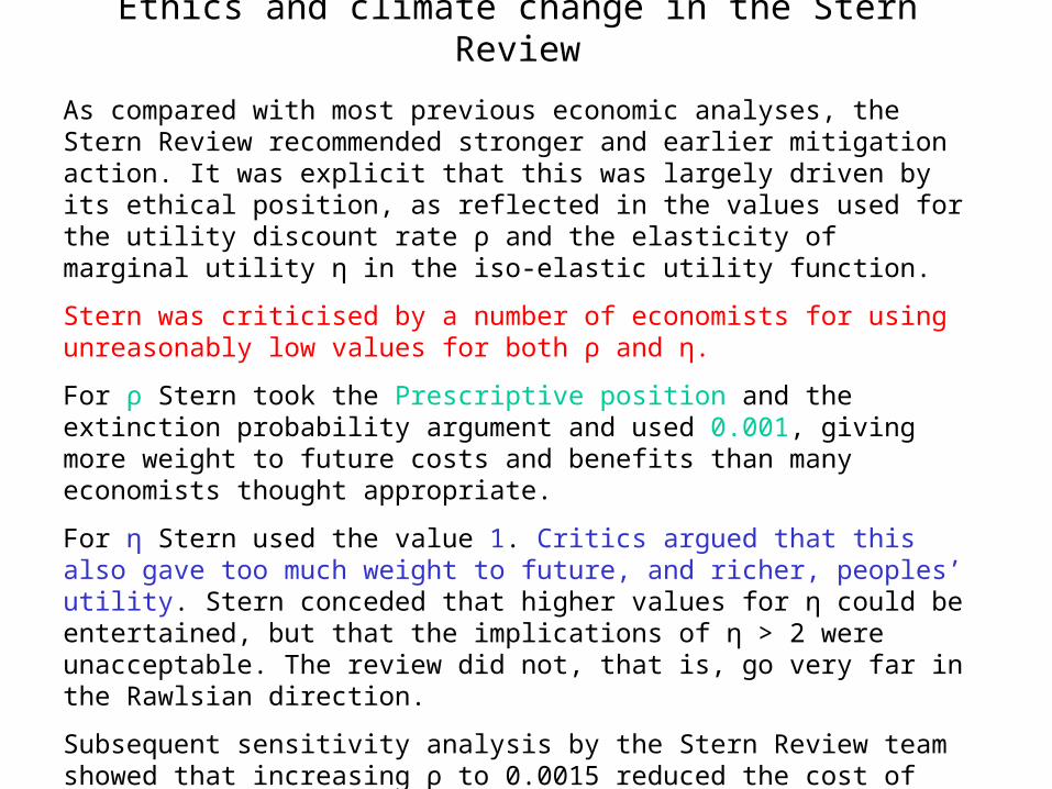
Ethics and climate change in the Stern Review
As compared with most previous economic analyses, the Stern Review recommended stronger and earlier mitigation action. It was explicit that this was largely driven by its ethical position, as reflected in the values used for the utility discount rate ρ and the elasticity of marginal utility η in the iso-elastic utility function.
Stern was criticised by a number of economists for using unreasonably low values for both ρ and η.
For ρ Stern took the Prescriptive position and the extinction probability argument and used 0.001, giving more weight to future costs and benefits than many economists thought appropriate.
For η Stern used the value 1. Critics argued that this also gave too much weight to future, and richer, peoples’ utility. Stern conceded that higher values for η could be entertained, but that the implications of η > 2 were unacceptable. The review did not, that is, go very far in the Rawlsian direction.
Subsequent sensitivity analysis by the Stern Review team showed that increasing ρ to 0.0015 reduced the cost of doing nothing from a 10.9% to 3.1% reduction in global per capita consumption forever, while increasing η reduced it to 3.4%.
The team did not see any need to change the main conclusion in favour of strong early action on mitigation.
Optimal growth: the model
Optimal growth is analysed as balance between the preferences/ethics of
Utility/consumption impatience - discounting
and the stylised fact of
The productivity of capital accumulation – a unit of consumption foregone now yields more than one unit of consumption in the future
dt)eU(CW
t
0t
ρtt
Maximisett C)Q(KK
tt C)Q(KK
Subject to
(3.18)
(3.19)
Optimal growth: a condition and its implications
K
C
C QρU
U
(3.20)
Along an optimal growth path, the proportional rate of change of marginal utility is equal to the difference between the utility discount rate, ρ, and the marginal product of capital, QK. ρ is a constant, QK falls as K increases.
Initially, QK is large and the rhs negative, which, given diminishing marginal utility has the lhs giving consumption increasing
The capital stock grows and QK declines. For QK = ρ the lhs goes to zero and consumption growth ceases.
Those alive early save for those alive later, who will be richer.
For ρ = 0, savings at every point in time would be higher, and capital accumulation would continue until QK went to zero.
For high ρ, early people would do less saving and accumulation and society remain poor despite the capacity to become rich
Optimal growth with non-renewable resource input
dt)eU(CWt
0t
ρt
t
tttC)R,Q(KK
tRS
dtRSt
0t t
Maximise
Subject to
(3.21)
(3.22a)
(3.22b)
(3.22c)
The implications of an ethical position – ρ > 0 - vary with circumstances
(a) The basic model
(b) Production uses inputs of a non-renewable resource
See also chapters 11, 14 and 19
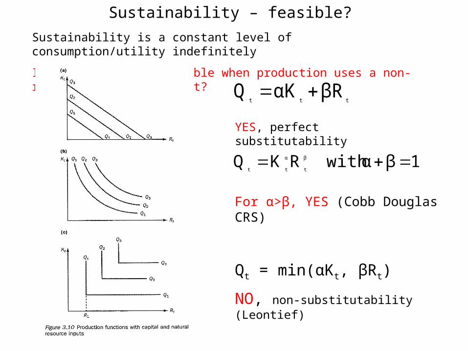
Sustainability – feasible?
Sustainability is a constant level of consumption/utility indefinitely
Is sustainability feasible when production uses a non-renewable resource input?
tttβRαKQ
1βαwithRKQ β
t
α
tt
For α>β, YES (Cobb Douglas CRS)
YES, perfect substitutability
Qt = min(αKt, βRt)
NO, non-substitutability (Leontief)
Sustainability – optimal?
Figure 3.9b is for the, Cobb Douglas, case where the production function means that sustainability is feasible, and the optimal consumption path is given by the maximisation of the present value of utility.
For this case maximising a Rawlsian intertemporal SWF,
W = Min(U0, U1,....)
would give constant consumption/utility as optimal.
C
t Figure 3.9b
The Hartwick Rule – a constraint on saving
For the, Cobb Douglas, case where constant consumption utility is feasible with a non-renewable resource used in production, following the Hartwick Rule gives constant consumption/utility.
The rule, a constraint, is that all of the rent arising from the extraction of the resource along an intertemporally efficient depletion programme must be saved and invested in the stock of reproducible capital, K.
In that case, the total value of the economy’s capital stock – K plus S – remains constant over time.
See Chapters 11, 14 and 19
Weak and strong sustainability Are not different kinds of sustainability – both refer to constant consumption/utility.
The distinction is between assumptions about substitution possibilities.
For weak sustainability the assumption is that these possibilities are as for the Cobb Douglas production function so that sustainability is feasible via the substitution of K for R.
For strong sustainability the assumption is that these possibilities are as for the Leontief production function.
More generally
Q = Q(L, KN, KH)
where KN is natural capital, and KH is human-made, or reproducible, capital and the weak/strong sustainability distinction is in terms of the substitution possibilities between KN and KH
Proponents of strong sustainability argue that KN must be non-declining, while for proponents of weak sustainability it is KH + KN that must be non-declining.
Ecologists on sustainability
Sustainability is a relationship between human economic systems and larger dynamic, but normally slower changing, ecological systems in which 1) human life can continue indefinitely, 2) human individuals can flourish, and 3)human cultures can develop, but in which effects of human activities remain within bounds, so as not to destroy the diversity, complexity, and function of the ecological life support system. (Costanza et al 1991)
In effect, ecologists judge the possibilities for substituting KH for KN to be limited, especially in regard to the ‘ecological life support system’.
Sustainability requires resilience – the maintenance of the ecosystem’s functional integrity in the face of exogenous disturbance. Resilience is not guaranteed by following standard economic criteria.
Ecologists, and strong sustainability proponents, argue for for explicit protection for ‘critical’ natural capital.