110 CHAPTER- 3 EXPERIMENTAL TECHNIQUES 3.0. INTRODUCTION: The relative permittivity (Є r ) or dielectric constant is defined as the dimensionless ratio of the permittivity of the dielectric to the permittivity of vacuum. It may be determined by obtaining the ratio of the capacitance (C) of a capacitor completely filled with the dielectric to the capacitance (C 0 ) of the capacitor filled with space. In practice, the permittivity of the dielectric is not normally compared with vacuum but with a reference gas or air. The capacitance is usually measured by a bridge method or resonance method. Bridge circuits have been described [1] and using either an absolute or non- absolute technique. The relative permittivity depends on frequency and the limiting value at zero frequency is termed as the ‘static relative permittivity’. In this section the values of Є r reported refer to the static relative permittivity. Є r plays an important role in the thermodynamics of electrolyte solutions. Determination of dielectric data of aqueous electrolytes of Sulphates, Chlorides and Nitrates of several transition metals were attempted by researchers with different techniques [2, 3, 4 ]. In the present study, transition metal Sulphates, Chlorides and Nitrates of Copper, Nickel, Manganese and Cobalt are selected and a new précise technique is developed in Engineering Physics Laboratory and Electronics and Communications Engineering Laboratory of Godavari Institute of Engineering and Technology, Rajahmundry, A.P, India, to determine dielectric constants of above aqueous electrolytes at 298K. This method is extended to calculate temperature variation of dielectric constants of Methanol, Benzene, Nitrobenzene and Water from 288K to 343K with the help of AN685 temperature sensor. The ‘Austrian made’ ANTON PAAR experimental setup, DSA-5000M is used for the very accurate determination of ultrasonic velocity, density, and Antonpaar’s Abbemate refractometer for evaluation of refractive index of the electrolyte solution of Copper Sulphate in binary solvent mixture of ethylene glycol and water in eleven compositions and six concentrations of the electrolyte at different temperatures from
Transcript
110
CHAPTER- 3
EXPERIMENTAL TECHNIQUES
3.0. INTRODUCTION:
The relative permittivity (Єr) or dielectric constant is defined as the dimensionless
ratio of the permittivity of the dielectric to the permittivity of vacuum. It may be
determined by obtaining the ratio of the capacitance (C) of a capacitor completely filled
with the dielectric to the capacitance (C0) of the capacitor filled with space. In practice,
the permittivity of the dielectric is not normally compared with vacuum but with a
reference gas or air. The capacitance is usually measured by a bridge method or
resonance method. Bridge circuits have been described [1] and using either an absolute or
non- absolute technique. The relative permittivity depends on frequency and the limiting
value at zero frequency is termed as the ‘static relative permittivity’. In this section the
values of Єr reported refer to the static relative permittivity. Єr plays an important role in
the thermodynamics of electrolyte solutions. Determination of dielectric data of aqueous
electrolytes of Sulphates, Chlorides and Nitrates of several transition metals were
attempted by researchers with different techniques [2, 3, 4 ]. In the present study,
transition metal Sulphates, Chlorides and Nitrates of Copper, Nickel, Manganese and
Cobalt are selected and a new précise technique is developed in Engineering Physics
Laboratory and Electronics and Communications Engineering Laboratory of Godavari
Institute of Engineering and Technology, Rajahmundry, A.P, India, to determine
dielectric constants of above aqueous electrolytes at 298K. This method is extended to
calculate temperature variation of dielectric constants of Methanol, Benzene,
Nitrobenzene and Water from 288K to 343K with the help of AN685 temperature sensor.
The ‘Austrian made’ ANTON PAAR experimental setup, DSA-5000M is used for
the very accurate determination of ultrasonic velocity, density, and Antonpaar’s
Abbemate refractometer for evaluation of refractive index of the electrolyte solution of
Copper Sulphate in binary solvent mixture of ethylene glycol and water in eleven
compositions and six concentrations of the electrolyte at different temperatures from
111
298K to 318K. A very accurate digital micro balance, Sartorius CPA -225D, is used to
determine the mass of the electrolyte.
3.1. Dielectric constant determination:-
The developed set up consists of (1) Dual 15 Volts Regulated Power Supply, (2)
F-V Converter and (3) Square wave generator.
Fig. 3.1.1. The block diagram of the experimental setup used in the determination of the
dielectric constant of the electrolytic systems.
3.1.1. DUAL 15 Volts Regulated Power Supply:-
The circuit digram shown in fig: 3.1.2 represents a 15V regulated dual power
supply [5]. The output of the circuit is +15Vand -15VDC. The 110V or 220V primary
and 18V center tap transformer is used to step down the mains voltage. The Diodes D1-
D4 perform the process of rectification which will convert 18V AC to18V DC. The
2200µF capacitor is used to filter the ripple in voltage coming from the diodes and other
capacitors in the circuit used for decoupling. The LM7815 and LM7915 are voltage
regulator Integrated Chips (ICs) which step down their input voltage to regulated dual
15V DC.
112
Fig 3.1.2.Circuit diagram of 15V regulated Dual power supply.The outputs of the circuit
are +15V to -15V.
Fig 3.1.3. DUAL 15 Volts 1 Amp Regulated Power Supply Connections on PCB.
113
3.1.2. Frequency to Voltage (F- V) Converter using the device ‘LM331’:
The device ‘LM331’ is a Frequency to Voltage Converter [6] supplied by
“Fairchild semiconductor” (www.fairchildsemi.com). KA331 can also used for this
pupose.
This circuit is designed to provide the output voltage, precisely proportional to the
applied input frequency. The device LM331 can be operated at power supplies as low as
4 V and can be used to chang output voltage from 0V to 10V. It is ideally suittable for
use in simple low cost circuit for analog to digital conversion, long term integration,
linear frequency modulation or demodulation,frequency to voltage conversion, and many
other similar functions.
Features of LM331:
1. Specific linearity (0.01% maximum),
2. Low power dissipation of 15mW at 5 V,
3. Wide range of full scale frequency 1Hz to 100KHz ,
4. Pulse output compatible with all logic forms,
5. Wide dynamic range, 100 dB minimum at 10 KHz full scale frequency.
Principle of operation of F- V Converter:
The LM331 is monolithic Integrated Circuit designed for accuracy and versatile
operation when applied as F to V converter. A simplified block diagram is shown if fig:
3. 1.4. It consists of switched current source, input comparator and one shot timer (R-S
Flip- flop).
114
Fig: 3. 1. 4. Simplified block diagram of LM331.
The frequency to voltage conversion is attained by differentiating the input
frequency using C-R network. The voltage comparator compares a positive input voltage
at pin- 7 to the voltage at pin- 6. The negative going edge of the resultant pulse trains at
pin- 6 makes the built in comparator circuit to trigger the timer circuit. The output of the
timer will turn on the switched current source for a period T= 1.1Rt Ct. During this
period, the current i will flow out of the switched current source and provide a fixed
amount of charge Q = i . t into the capacitor CL. The current flowing into CL is exactly
iavg = i (1.1Rt Ct) f. At any instant, the current flowing out of the pin- 1 is proportional to
input frequency. Hence the output voltage is proportional to input frequency available
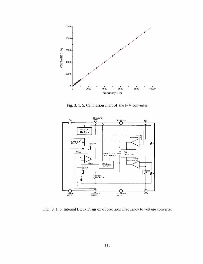
across the load resistance RL. The graph between input frequency (Hz) and output voltage
( mV) is linear as shown in fig: 3.1.5.
Calibration of the F-V converter:
The F-V converter was precisely calibrated with the standard signal generator and
graph was plotted between voltage and frequency. This resultant graph is a straight line
with 0.01% linearity.
115
Fig. 3. 1. 5. Calibration chart of the F-V converter.
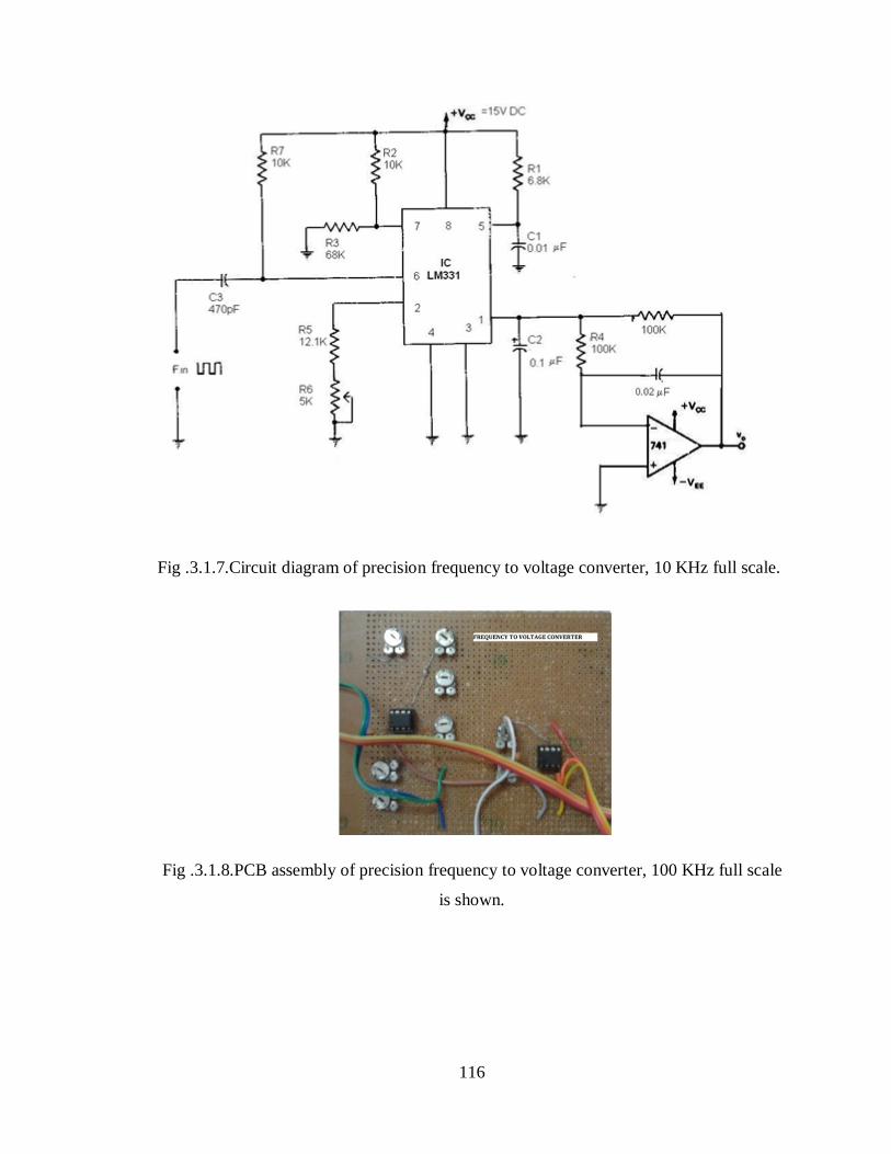
Fig. 3. 1. 6. Internal Block Diagram of precision Frequency to voltage converter
116
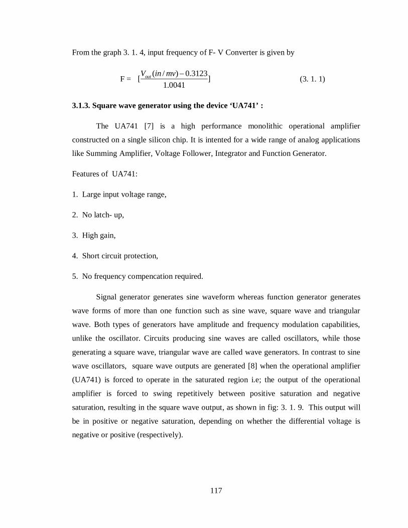
Fig .3.1.7.Circuit diagram of precision frequency to voltage converter, 10 KHz full scale.
Fig .3.1.8.PCB assembly of precision frequency to voltage converter, 100 KHz full scale
is shown.
117
From the graph 3. 1. 4, input frequency of F- V Converter is given by
F = ( / ) 0.3123[ ]
1.0041outV in mv
(3. 1. 1)
3.1.3. Square wave generator using the device ‘UA741’ :
The UA741 [7] is a high performance monolithic operational amplifier
constructed on a single silicon chip. It is intented for a wide range of analog applications
like Summing Amplifier, Voltage Follower, Integrator and Function Generator.
Features of UA741:
1. Large input voltage range,
2. No latch- up,
3. High gain,
4. Short circuit protection,
5. No frequency compencation required.
Signal generator generates sine waveform whereas function generator generates
wave forms of more than one function such as sine wave, square wave and triangular
wave. Both types of generators have amplitude and frequency modulation capabilities,
unlike the oscillator. Circuits producing sine waves are called oscillators, while those
generating a square wave, triangular wave are called wave generators. In contrast to sine
wave oscillators, square wave outputs are generated [8] when the operational amplifier
(UA741) is forced to operate in the saturated region i.e; the output of the operational
amplifier is forced to swing repetitively between positive saturation and negative
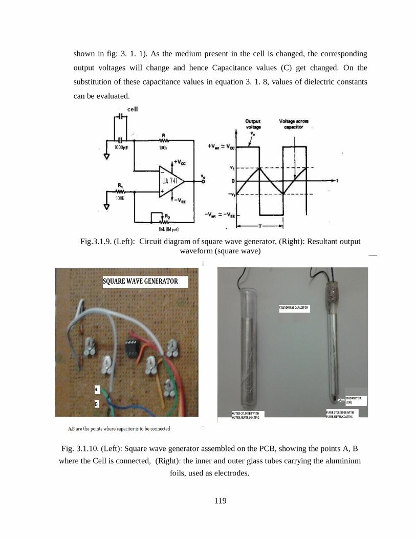
saturation, resulting in the square wave output, as shown in fig: 3. 1. 9. This output will
be in positive or negative saturation, depending on whether the differential voltage is
negative or positive (respectively).
118
The time period of the output waveform of the square wave generator is given by
1 2
2
(2 )2 ln[ ]R RT RCR
(3. 1. 2)
Where the values of the resistances used in the circuit are taken as:
R = 100 KΩ, R1 = 100KΩ and R2 = 116KΩ
The output frequency of the circuit is given by
1 1 2 ln [(2R1+R2)/ (R2)]outF RCT
(3. 1. 3)
In the experiment, value of R2 is taken as 1.16R1, then
1[ ](2.0044)outF
RC
(3. 1. 4)
This output frequency of the square wave generator is taken as input for F- V converter,
hence from equations (3. 1. 1), (3. 1. 4)
( / ) 0.3123[ ]1.0041
outV in mv = 1[ ]
(2.0044)RC
Which gives
0.5010[ ( ( )) 0.3123]out
CR V inmv
(3.1.5)
where C is resultant value of capacitance of the cell (Ccell) and 1000pF connected in
parallel in Fig: 3.1. 9., i. e; C = Ccell + 1000 pF,
which gives, Ccell = 1000pF – C (3. 1. 6)
here, C can be calculated from equation 3.1.5 by taking R = 100 KΩ and Vout (in milli-
volt) from a digital milli- voltmeter connected in the circuit (Voltage measuring device,
119
shown in fig: 3. 1. 1). As the medium present in the cell is changed, the corresponding
output voltages will change and hence Capacitance values (C) get changed. On the
substitution of these capacitance values in equation 3. 1. 8, values of dielectric constants
Fig. 3.1.10. (Left): Square wave generator assembled on the PCB, showing the points A, B where the Cell is connected, (Right): the inner and outer glass tubes carrying the aluminium
foils, used as electrodes.
120
3.1.4. Fabrication of the cell for Capacitance measurement:
Fig: 3.1.11. Cell for Capacitance measurement.
The cell is designed to cater to the following precautions:
(1) To minimize the temperature gradient across the test fluid,
(2) To control the stray field effects arising from an inhomogeneous field
configuration,
(3) To reduce spurious contributions due to the polarization impedance at the
interface between the electrodes and the sample surface,
(4) The cell has to be a volume independent with parallel concentric cylindrical
electrodes filled with the liquid at homogenous temperature.
(5) The virtual isolation of the electrodes from the liquid by using the borosilicate
glass tube into which the liquid is taken, ensures, unwanted chemical interactions
at electrodes with the liquid under study.
121
The cell for Capacitance measurement is shown in Fig: 3. 1. 10 and 3. 1. 11. It is
made-up of glass tubes having an inner cylindrical electrode of diameter 1.494x10⁻²m (a2)
and an outer cylindrical electrode of diameter 2.533x10⁻² m (b1). Thin aluminium foils are
taken as electrodes. The two electrodes are mounted coaxially with a uniform gap of
2.3417x10⁻⁴ m2. The liquid (chosen electrolyte) was taken into the cylindrical cell
(medium), into the space between the inner and outer glass tubes, and the leads from the
electrodes were connected to the square wave generator at points A and B as shown in
fig: 3. 1. 10 (Left).
The expression for capacitance of the cylindrical cell is given by the equation
0
2 1 21 2 1
1 2 1
(2 )
[(ln ) / ) (ln( ) / ) (ln( ) / )]cell
LC a b bk k ka a b
(3. 1. 7)
Where, L is the length of the electrodes taken in the experiment, equal to 10.05×10⁻²m,
a1 is inner diameter of inner cylinder, equal to 1.494 ×10⁻²m,
a2 is outer diameter of inner cylinder, equal to 1.8 ×10⁻²m,
b1 is inner diameter of outer cylinder, equal to 2.266 ×10⁻²m,
b2 is outer diameters of outer cylinder, equal to 2.533×10⁻²m.
All diameters are measured with the help of Vernier Callipers whose least count is
0.01×10⁻²m,
k1, k2 are the dielectric constants of the borosilicate glass and the medium taken in the cell
respectively. The value of k1 is 4.6, taken from the literature of the manufacturer [9].
and the dielectric constant, k2 of the medium taken in the cell is given by reducing 3. 1. 7,
2 1 1( )med air
xkx
C C
(3. 1. 8)
where X is constant of the cell, depends upon dimensions of the cell, given by
122
0
1
2
[ln( ) / 2 ]bX La
(3.1. 9)
The value of X is 412.6704 × 10⁸ which is so sensitive that fourth digit after
decimal may change for every set of experimental values due to fluctuations in
temperature and moisture present in the atmosphere. It is necessary to calculate before
commencement of the each set of experimental values. Cair = 18.9581pF which is
constant throughout the experiment.. Capacitance values Cmed ( in pF) values are
tabulated along with dielectric constants of chosen electrolytic solutions under study in
the chapter ‘Results and Discussions’.
3.1.5.. Standardization of the cell and experimental precautions:
The liquids chosen for the standardization of the cell for capacitance measurement
are listed in Table 3.1.1. The Dielectric Constant data is taken from standard literature
source [10]. The experimental dielectric constants with corresponding capacitance values
obtained are tabulated in the same table. All the important precautions for the
maintenance [11, 12 and 13] of the purity of the liquids used are very carefully
implemented. High Purity Chemicals, of Merck-make are used throughout the
experimentation. The water is double distilled. The Borosilate glass ware used in the
experimentation is cleaned thoroughly in distilled water, dried and then used between two
consecutive measurements.
123
Table. 3. 1. 1. Details of the liquids chosen for the standardization of the cell used for the
capacitance measurement and their experimental Dielectric Constants.
Dielectric medium Capacitance C (in pF )
Static Dielectric
constant (Experimental)
Static Dielectric constant
(Literature)
Carbon Tetra chloride
33.3101 2.2290 2.2380
Toluene 35.3608 2.4600 2.4680
Glycerol 80.3108 42.540 42.500
Ethyl Benzene 34.5807 2.370 2.400
Water 83.2815 78.369 78.360
Acetyl Acetone 76.4010 25.690 25.700
3.2. Dielectric constant determination with temperature variation using AN685:
A simple relationship between dielectric constant of mixed solvents with solvent
composition and temperature was proposed by Abolghasem Jouybanet.al.[14], Neeta
Sarma et.al [15] studies used an electronically controlled temperature bath with an
accuracy of 0.002 K in their work.
For pure liquids, Wear [16] reported that Sargent Oscillometer technique is good
enough but not compatible for temperature controlled measurements. Even though this
method is a development for the Oscillometer method, its accuracy of measurement of
temperature is restricted, mainly because, a temperature bath is used to regulate the
temperature by a liquid circulation technique. Ahlawat, Venkatesh, Haynes, P. K. Yu
[17], mentioned other techniques of interest, but for specialised applications.
Procedure:
In the technique presented in this study, a precise resistance tool kept at the same
temperature as the medium, for the determination of the dielectric constants of Water,
124
Benzene, Methanol and Nitrobenzene at different temperatures. This is possible because
a small thermistor of type AN685 [18] is held inside the dielectric cell as shown in fig:
3.1.10 (Right) and 3.1.11 above. This makes the environment around the thermistor to be
isothermal. The equipment used in present study has the ability to determine the
temperature at the place of interaction. This set up enables the temperature measurement
by the thermistor to an accuracy of 0.0001K. The resistance related to the temperature on
a logarithmic scale is shown in the figure 3. 2. 2. Since the thermistor is held in the very
close proximity to the place of interaction, the temperature measurement is very precise.
Theoretically the equation for the temperature dependence, according to Wear [16] is
given by
(3. 2. 1)
in which ε is the Dielectric Constant , T is the absolute temperature , and L and ε0 are
constants for a given solvent. The theoretical values of the ‘ ε ‘, of above mentioned
solvents has been evaluated, using this equation. The values of the constants for the
chosen solvents are given in the table 3. 2. 1. The experimental dielectric constant data of
these solvents at different temperatures along with corresponding values of capacitances
are presented in the chapter ‘Results and Discussions’. The procedure for experimental
dielectric constant determination is same as detailed in article 3. 1, except for the study of
temperature variation being the addition.
Fig: 3. 2. 1. Electrolytic cell placed in the thermocol box.
125
To study temperature variation of resistance, the thermistor AN 685 is carefully
lodged into the inner cylindrical tube of the cell. The liquid under investigation is heated
up to 850C and is transferred into the cell. Now the cell is placed into a thermocol box of
suitable shape and size as shown in the fig: 3. 2. 1. The top of the box is kept open to the
atmosphere to facilitate slow and gradual cooling. Since the thermistor is a resistive
element, current excitation is required, as shown in the fig: 3. 2. 2(Right). The potential
difference across the thermistor is determined using digital milli- voltmeter. The current
passing through the thermistor is determined using the digital micro- ammeter (not shown
in the diagram). The ratio of instantaneous values of potential difference and current
gives the instantaneous values of resistance of the thermistor. The temperature
corresponding to this resistance is noted down from the table 3. 2. 3.
Table: 3. 2. 1. Constants of Solvents used for calculation of Dielectric Constants
Solvent Value of ε0 L x 103
Benzene 2.95 0.876
Methanol 157.6 5.39
Nitrobenzene 164.7 5.21
Water 311.17 4.63
A similar method is [19] is used in literature for the water-ethanol system also.
The water-methanol data reported by Wear observed discrete departure between theory
and experiment. This is expected , as per the observations of other prominent findings of
different techniques, like U-V visible spectrophotometry, Ion selective electrode
potentiometry, Dielectric relaxation spectroscopy, and titration colorimetry.
3.2.1. Theory:
The thermistor is operated in the Temperature- Resistive mode. Fig: 3. 2. 2 (Left)
illustrates the high degree of non- linearity of thermistor element. The non- linear
response of thermistor can be corrected in software with an empirical third order
polynomial, called Steinhart-Hart thermistor equation. This equation is an approximation
126
and can replace the exponential expression for a thermistor. Steinhart-Hart thermistor
equation is give by,
30 1 3
1[ ln( ) ln( )]T T
TA A R A R
(3. 2. 2)
Where, 30 1 3ln( ) [ / ] [ / ]TR B B T B T
T is the temperature of the thermistor in Kelvin and A0, A1, A3, B0, B1, and B3 are
constants provided by the manufacturer, and RT is the thermistor resistance at
temperature, T. With a typical thermistor, this third order linearization formula provides
+ 0.10C accuracy over the full temperature range.
In precision temperature measurement of environments, the thermistor is used in a
“zero power” condition. In this condition, the power consumption of the thermistor has a
negligible effect on the elements resistance. The graph 3. 2. 2(Left) shown below is 10kΩ
Negative Temperature Coefficient (NTP) thermistor resistance-versus-temperature,
clearly indicates the accuracy of the measurements.
Fig 3.2.2: (Left): The Temperature Vs Resistance Calibration Plot, (Right): Excitation of
thermistor by a precision constant current source.
127
Table: 3. 2. 3. Resistive changes with temperature of a Beta THERM NTC thermistor in
its zero power modes.
Temp (0C) Resistance (Ω) Temp (0C) Resistance (Ω)
0 32650.8 55 2985.1
5 25398.5 60 2487.1
10 19903.5 65 2082.3
15 15714.0 70 1751.6
20 12493.7 75 1480.12
25 10000 80 1256.17
30 8056.0 85 1078.58
35 6530.1 90 916.11
40 5324.9 95 786.99
45 4366.9 100 678.63
50 3601.0 105 587.31
3.3. Ultrasonic Velocity, Density and Refractive Index Determination:
Most of the measurements of velocity of ultrasonic waves in liquids since 1932
have involved optical diffraction techniques. The advantage of these methods is that
progressive waves can be used. But there are a number of limitations for continuous wave
methods. Streaming and sample heating are some of the disadvantages. But it is possible
with modern electronic equipment to measure with sufficient accuracy, the short time of
passage of a pulse through a liquid to estimate its velocity, and the height of the echoes
can be used to measure attenuation. The notions that propagation of ultrasonic pulses
through a medium can be made use of in the investigation of physical properties of the
medium have led to the development of various methods for measuring velocity and
attenuation. One such method is by the usage of a vibrating tube made to resonate to an
external excitation. The Austrian made ANTONPAAR experimental setup, DSA-5000M
is used for the very accurate determination of ultrasonic velocity and density.
128
António José Queimada [20] determined Liquid density with an Antonpaar DMA
58 setup, based on the vibrating U- tube method. It measures the oscillating period of U-
tube filled with sample that is automatically converted to liquid density after proper
calibration.
Amalia Ştefaniu and M. Rogalski [21], reported density, viscosity and refractive
index determinations followed by apparent molar volumes and the transfer volumes of
amino acid in aqueous electrolyte solutions evaluations.
Stoppa, Buchner and Hefter [22] measured Densities, with an uncertainty of ±0.05
kgm−3 using a vibrating tube densimeter (Anton Paar, Graz, Austria, DMA60/601HT).
An improved version is used in this present study.
The Antonpaar, DMA 5000 Generation M is the latest and the most accurate
density meter for liquids,with most reliable and highly reproducible results. It has a
Filling Check provision for the automatic detection of filling errors like the presence of
air bubbles in the liquid column of the U-tube. The filling process of the sample can be
checked by an image displayed on the screen. The equipment used measures the
oscillating period of U-tube filled with sample that is automatically converted to liquid
density after proper calibration. It is a two in one instrument equipped with a sound
velocity cell and a density cell. Two density standards have to be selected for calibration,
at each temperature. In this work, air and distilled water were used as calibrating fluids.
This instrument can be operated from 263.15 K up to 343.15 K, with a built-in high-
precision platinum Resistance thermometer and it uses approximately 3ml of sample,
injected with a syringe, to be experimented upon. The temperature is kept constant with a
built-in Peltier element that can control temperature in the cell within ± 0.005 K. The
temperature is displayed with an accuracy of± 0.01 K and density values within ± 10-2
Kg·m-3. Due to high temperature dependence of the density and velocity of sound, the
measuring cells have to be thermostated precisely.
Antonpaar’s “Abbemate refractometer” supplied by the manufacturer as a part
of the total set up is used for determination of the refractive index of the Ionic liquid. It
provides quick and reliable refractive index measurements at multiple wavelengths
129
(optional) for all kinds of samples, and no sample preparation is necessary. High-
precision measurement in a wide range of refractive indices from 1.30 nD to 1.72 nD is
possible with this. Measurements at multiple wavelengths and high-temperature
measurements up to 110 °C are possible with optional gadgets, with a required sample
volume of only a few micro- lifers. It is a Non-destructive method without any chemical
reaction occurring during the determination.
3. 3. 1. Special features:
1. The equipment is very sophisticated, and can automatically change the
temperature in chosen steps. It is very precise and accurate for sound velocity and
density measurements of the sample in one cycle.
2. A very significant feature of the Antonpaar set up is the accurate and fast results
with a small sample volume of nearly 5ml ( for three parameter measurement)for
a set of pre-programmed temperatures, the changing of which in a cycle of
measurements is taken care of by the instrument, with a measuring time of nearly
1- 4 minutes per sample.
3. The set-up is provided with software that is capable of memorizing and displaying
of Sound Velocity, Density and Refractive Index, Temperature, as well as all
calculated properties, with a proper labelling of the specimens in a sequential
order, on the screen of a Touch Screen Electronic Monitor (with simultaneous
recording into hard disc memory). The data can be drawn out at leisure later in
any programmable format of the users choice.
4. Simultaneous and automatic filling and cleaning of the cells, and detection of the
filling errors, if any, is a special feature that ensures insulation from possible
human errors.
130
3. 3. 2. Measuring range and Accuracy:
Ultrasonic velocity: 1000- 2000 m/sec with accuracy of 0.5 m/sec
Density: 0- 3 gram/cc with accuracy of 0. 000005 gram/cc
Temperature: 0- 700 C with accuracy of 0.030C.
Refractive Index: 1.30 nD - 1.72 nD with accuracy of ±0.0001.
3. 3. 3. Basic principles of working:
(i) Ultrasonic velocity measuring principle:
The sample is introduced into the measuring cell that is bordered by an ultrasonic
transmitter on one side. The transmitter sends sound waves of known period through the
sample. The velocity of sound can be calculated by determining of the period of received
sound waves and by considering the distance between transmitter and receiver.
5[1 (1.6 )10 ]/[ . ]PU L T c e
X
(3. 3. 1)
Where, L = Original length of the sound waves
∆T = Temperature deviation to 20oC
P = Oscillation period of the received sound waves
X =divisor, 512
c = Operator constant for sound velocity& e = correction term for temperature
(ii) Density measuring principle:
The sample is introduced into a borosilicate glass tube that is being excited to
vibrate at its characteristic frequency electronically. This frequency changes depending
on the density of the sample. Through a precise determination of the characteristic
frequency and a mathematical conversion, the density of the sample can be measured
using the expression,
131
Density = 21 2A BK Q e K e (3. 3. 2)
Where, KA and KB - apparatus constants,
Q - Quotient of the period of oscillation of the U- divided by the period
of oscillation of the reference oscillator,
e1, e2 - correction terms for temperature, viscosity and non- linearity.
3.3.4. Usage of chemicals and preparation of ionic liquids of different concentrations
and compositions in aqueous Ethylene Glycol:
CuSO4 (5H2O), Ethylene Glycol both are analytical reagents(AR) purchased from
Merck with Assay 99.8%- 102% and 99.8% respectively. The copper sulphate used is in
the form of a penta- hydrate (molecular weight 249.69). Ethylene Glycol is used as binary
solvent mixture with water. The mixtures of the desired composition were prepared by
weighing on a very accurate digital micro balance, Sartorius CPA -225D, to determine
the mass of the electrolyte with a precision of ±0.0001 g. In order to prepare the solutions
under investigation in the form of aqueous ionic liquids, a stock solution of 50ml of each
concentration is prepared according to scheme presented in Appendix- A at the end of
the thesis. This stock solution is added to ethylene glycol (redistilled) to makeup ionic
liquids of the required composition. Since we required 5ml of each composition, the
mixing is done according to the prepared scheme. Each composition of 5ml is injected
into the setup using a syringe. However these compositions are prepared well before the
experiment to ensure that the mixing of the components of each composition is complete.
These compositions are carefully preserved in a refrigerator. The compositions are
allowed to get the room temperature of the laboratory by keeping them outside the
refrigerator at least for 90 minutes, before syringing them into the Antopaar setup.
132
(a) (b)
(c) (d)
133
(e) (f)
FIG: 3. 3. 1. ANTON PAAR Setup used in the acoustic, densimetric and Refraction
studies.
(a) Abbes Refractometer (b) Acoustic Velocity and Density measuring unit (c) Probe
used for the measurement of Acoustic Velocity and Density (d) Digital electronic balance
(e) Display on the monitor during refractive index measurement (f) Refractometer
connection point.
134
References
[1] Vaughan, Smyth and Owles, Techniques of Chemistry, 1, Physical Methods of
Chemistry, Part IV, edited by Weissberger and Rossiter, pp 351, Viley- Inter
science, New YorK, (1972).
[2] Brahmajirao, Indian J. pure and Appl. Phys., 14, pp 643, (1976).
[3] Chen, Glenn, Hefter and Richard Buchner; Journal of Solution Chemistry, 34(9),
(2005).
[4] C.Akhilan, Rohman, Hefter and Buchner, J. Phys. Chem., 110(30), 14961-14970,