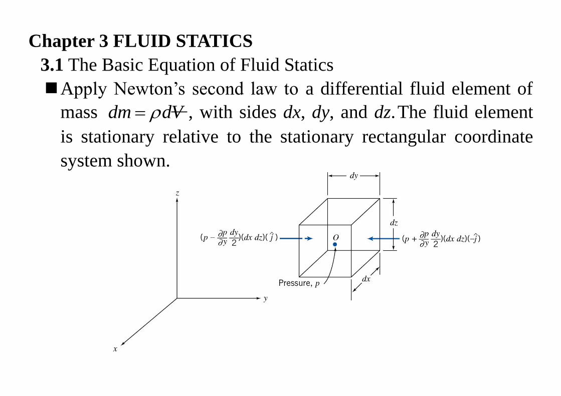
Chapter 3 FLUID STATICS 3.1 The Basic Equation of Fluid Statics Apply Newton’s second law to a differential fluid element of mass dm dV , with sides dx, dy, and dz. The fluid element is stationary relative to the stationary rectangular coordinate system shown.
Transcript
Chapter 3 FLUID STATICS
3.1 The Basic Equation of Fluid Statics
Apply Newton’s second law to a differential fluid element of
mass dm dV , with sides dx, dy, and dz. The fluid element
is stationary relative to the stationary rectangular coordinate
system shown.
Two general types of forces may be applied to a fluid: body
forces and surface forces. The only body force that must be
considered in most engineering problems is due to gravity. In
some situations body forces caused by electric or magnetic
fields might be present; they will not be considered in this text.
B SdF dF dF dma dVa
For a differential fluid element, the body force is
BdF gdm g dV
In Cartesian coordinates dV dxdydz , so
BdF gdxdydz
In a static fluid there are no shear stresses, so the only surface
force is the pressure force. Pressure is a scalar field, p=p(x, y,
z); in general we expect the pressure to vary with position
within the fluid.
Let the pressure be p at the center, O, of the element. To
determine the pressure at each of the six faces of the element,
we use a Taylor series expansion of the pressure about point O.
The pressure at the left face of the differential element is
2 2
L L
p p dy p dyp p y y p p
y y y
The pressure on the right face of the differential element is
2 2
R R
p p dy p dyp p y y p p
y y y
The pressure force on each face acts against the face. A
positive pressure corresponds to a compressive normal stress.
Collecting and canceling terms, we obtain
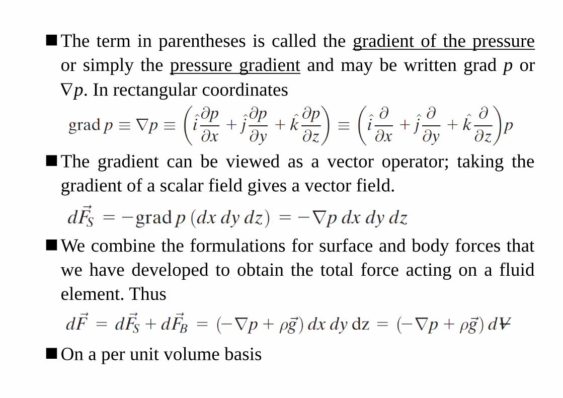
The term in parentheses is called the gradient of the pressure
or simply the pressure gradient and may be written grad p or
p. In rectangular coordinates
The gradient can be viewed as a vector operator; taking the
gradient of a scalar field gives a vector field.
We combine the formulations for surface and body forces that
we have developed to obtain the total force acting on a fluid
element. Thus
On a per unit volume basis
For a fluid particle, Newton’s second law gives
F adm a dV . For a static fluid, 0a . Thus
We obtain
The physical significance of each term is
This is a vector equation, which means that it is equivalent to
three component equations that must be satisfied individually.
The component equations are
If the coordinate system is chosen with the z axis directed
vertically upward, then gx=0, gy=0, and gz=-g. Under these
conditions, the component equations become
It indicates that, under the assumptions made, the pressure is
independent of coordinates x and y; it depends on z alone.
Thus since p is a function of a single variable, a total
derivative may be used instead of a partial derivative. With
these simplifications, above equation finally reduce to
Restrictions: (1) Static fluid.(2) Gravity is the only body
force.(3) The z axis is vertical and upward.
is the specific weight of the fluid. This equation is the basic
pressure-height relation of fluid statics.
The pressure values must be stated with respect to a reference
level. If the reference level is a vacuum, pressures are termed
absolute. Most pressure gages indicate a pressure
difference—the difference between the measured pressure and
the ambient level (usually atmospheric pressure). Pressure
levels measured with respect to atmospheric pressure are
termed gage pressures.
For example, a tire gage might indicate 207 kPa; the absolute
pressure would be about 308 kPa. Absolute pressures must be
used in all calculations with the ideal gas equation or other
equations of state.
3.2 The Standard Atmosphere
Scientists and engineers sometimes need a numerical or
analytical model of the Earth’s atmosphere in order to simulate
climate variations to study, for example, effects of global
warming.
There is no single standard model. An International Standard
Atmosphere (ISA) has been defined by the International Civil
Aviation Organization (ICAO); there is also a similar U.S.
Standard Atmosphere.
The temperature profile of the U.S. Standard Atmosphere is
shown in the following figure.
Sea level conditions of the U.S. Standard Atmosphere are
summarized in the table.
3.3 Pressure Variation in a Static Fluid
We proved that pressure variation in any static fluid is
described by the basic pressure height relation.
dpg
dz
Although ρg may be defined as the specific weight, γ, it has
been written as ρg in above equation to emphasize that both ρ
and g must be considered variables.
For most practical engineering situations, the variation in g is
negligible. Only for a purpose such as computing very
precisely the pressure change over a large elevation difference
would the variation in g need to be included. Unless we state
otherwise, we shall assume g to be constant with elevation at
any given location.
Incompressible Liquids: Manometers
For an incompressible fluid, ρ=constant. Then for constant
gravity,
constantdp
gdz
If the pressure at the reference level, z0, is designated as p0,
then the pressure, p, at level z is found by integration:
0 0
0 0 0
p z
p zdp gdz p p g z z g z z
For liquids, it is often convenient to take the origin of the
coordinate system at the free surface (reference level) and to
measure distances as positive downward from the free
surface.
With h measured positive downward, we have
z0-z=h
And obtain
0p p p gh
Above equation indicates that the pressure difference
between two points in a static incompressible fluid can be
determined by measuring the elevation difference between
the two points. Devices used for this purpose are called
manometers.
Ex. 3.1 Systolic and Diastolic Pressure: Normal blood pressure
for a human is 120/80 mm Hg. By modeling a sphyg-
momanometer pressure gage as a U-tube manometer, convert these
pressures to kPa.
Given: Gage pressures of 120 and 80 mm Hg.
Find: The corresponding pressures in kPa.
Notes: # Two points at the same level in a continuous single
fluid have the same pressure. # In manometer problems we
neglect change in pressure with depth for a gas: ρgas << ρliquid. #
This problem shows the conversion from mm Hg to kPa: 120
mm Hg is equivalent to about 2.32 psi. More generally, 1 atm
=14.7 psi= 101 kPa= 760 mm Hg.
The sensitivity of a manometer is a measure of how sensitive
it is compared to a simple water-filled U-tube manometer.
Specifically, it is the ratio of the deflection of the manometer
to that of a water-filled U-tube manometer, due to the same
applied pressure difference Δp.
Ex.3.2 Analysis of Inclined-Tube Manometer: An inclined-tube
reservoir manometer is constructed as shown. Derive a general
expression for the liquid deflection, L, in the inclined tube, due to
the applied pressure difference, Δp. Also obtain an expression for
the manometer sensitivity, and discuss the effect on sensitivity of D,
d, θ, and SG.
Given: Inclined-tube reservoir manometer.
Find: Expression for L in terms of Δp. General expression for
manometer sensitivity. Effect of parameter values on sensitivity.
2
1
sinl
Ls
h d
D
, Gage Liquid (0.8), Diameter Ratio
(0.1), Inclination Angle (10 degree).
Combining the best values (SG=0.8, d/D=0.1, and θ=10
degrees) gives a manometer sensitivity of 6.81. Physically this
is the ratio of observed gage liquid deflection to equivalent
water column height. Thus the deflection in the inclined tube is
amplified 6.81 times compared to a vertical water column.
With improved sensitivity, a small pressure difference can be
read more accurately than with a water manometer, or a
smaller pressure difference can be read with the same
accuracy.
Students sometimes have trouble analyzing multiple-liquid
manometer situations. The following rules of thumb are useful:
1. Any two points at the same elevation in a continuous region
of the same liquid are at the same pressure.
2. Pressure increases as one goes down a liquid column
(remember the pressure change on diving into a swimming
pool).
To find the pressure difference Δp between two points
separated by a series of fluids,
i i
i
p g h
Ex. 3.3 Multiple-Liquid Manometer: Water flows through pipes
A and B. Lubricating oil is in the upper portion of the inverted U.
Mercury is in the bottom of the manometer bends. Determine the
pressure difference, pA-pB, in units of kPa.
Given: Multiple-liquid manometer as shown.
Find: Pressure difference, pA-pB, in kPa.
Atmospheric pressure may be obtained from a barometer, in
which the height of a mercury column is measured.
Although the vapor pressure of mercury may be neglected, for
precise work, temperature and altitude corrections must be
applied to the measured level and the effects of surface tension
must be considered.
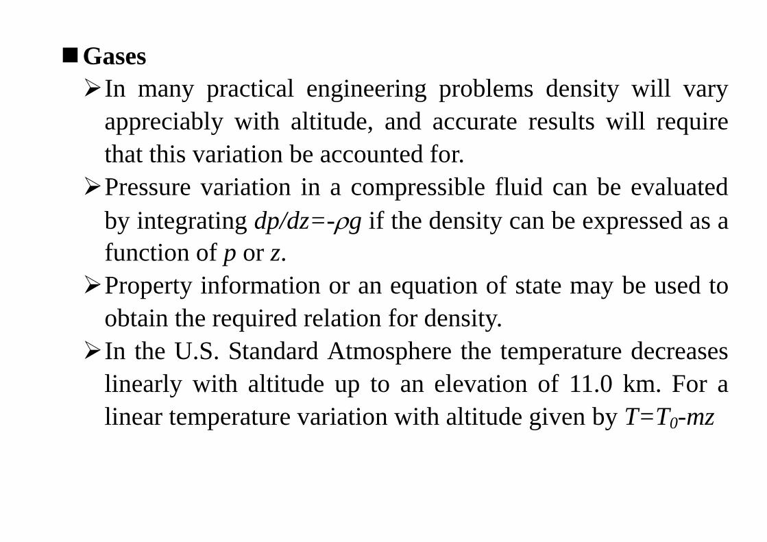
Gases
In many practical engineering problems density will vary
appreciably with altitude, and accurate results will require
that this variation be accounted for.
Pressure variation in a compressible fluid can be evaluated
by integrating dp/dz=-g if the density can be expressed as a
function of p or z.
Property information or an equation of state may be used to
obtain the required relation for density.
In the U.S. Standard Atmosphere the temperature decreases
linearly with altitude up to an elevation of 11.0 km. For a
linear temperature variation with altitude given by T=T0-mz
0
pg pgdp gdz dz dz
RT R T mz
Separating variables and integrating from z=0 where p=p0 to
elevation z where the pressure is p gives
0 00 0 0
/ /
0 0
0 0
ln ln 1
1
p z
p
g mR g mR
dp gdz p g mz
p R T mz p mR T
mz Tp p p
T T
Ex. 3.4 Pressure and Density Variation in the Atmosphere: The
maximum power output capability of a gasoline or diesel engine
decreases with altitude because the air density and hence the mass
flow rate of air decrease. A truck leaves Denver (elevation 1610 m)
on a day when the local temperature and barometric pressure are
27C and 630 mm of mercury, respectively. It travels through Vail
Pass (elevation 3230 m), where the temperature is 17C.
Determine the local barometric pressure at Vail Pass and the
percent change in density.
Given: Truck travels from Denver to Vail Pass. Denver: z=1610 m,
p=630 mm Hg., T=27C; Vail Pass: z=3230 m, T=17C.
Find: Atmospheric pressure at Vail Pass. Percent change in air
density between Denver and Vail.
This Example shows use of the ideal gas equation with the
basic pressure-height relation to obtain the change in pressure
with height in the atmosphere under various atmospheric
assumptions.
3.4 Hydraulic Systems
Hydraulic systems are characterized by very high pressures,
so by comparison hydrostatic pressure variations often may be
neglected.
Automobile hydraulic brakes develop pressures up to 10 MPa
(1500 psi); aircraft and machinery hydraulic actuation systems
frequently are designed for pressures up to 40 MPa (6000 psi),
and jacks use pressures to 70 MPa (10,000 psi).
Although liquids are generally considered incompressible at
ordinary pressures, density changes may be appreciable at high
pressures.
Bulk moduli of hydraulic fluids also may vary sharply at high
pressures. In problems involving unsteady flow, both
compressibility of the fluid and elasticity of the boundary
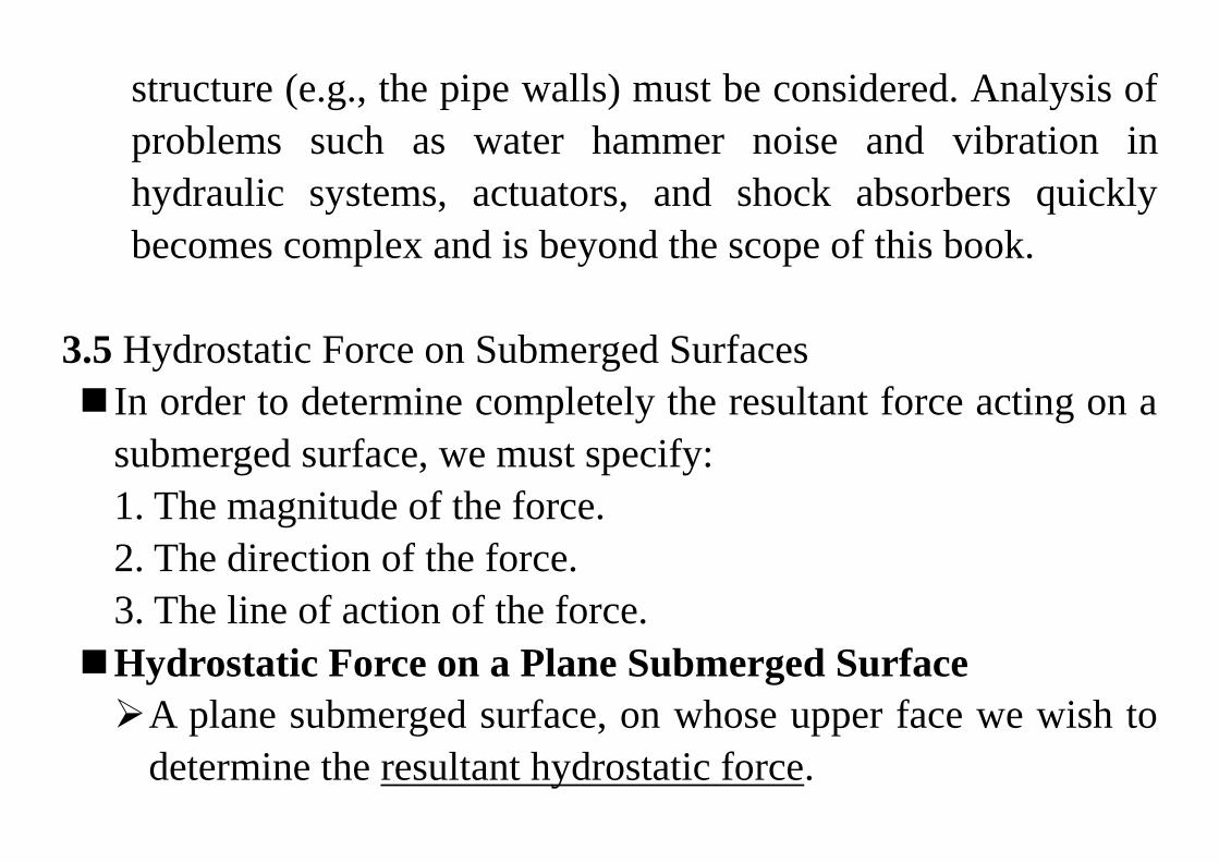
structure (e.g., the pipe walls) must be considered. Analysis of
problems such as water hammer noise and vibration in
hydraulic systems, actuators, and shock absorbers quickly
becomes complex and is beyond the scope of this book.
3.5 Hydrostatic Force on Submerged Surfaces
In order to determine completely the resultant force acting on a
submerged surface, we must specify:
1. The magnitude of the force.
2. The direction of the force.
3. The line of action of the force.
Hydrostatic Force on a Plane Submerged Surface
A plane submerged surface, on whose upper face we wish to
determine the resultant hydrostatic force.
The coordinates are important: They have been chosen so that
the surface lies in the xy plane, and the origin O is located at
the intersection of the plane surface (or its extension) and the
free surface.
The magnitude of the force FR, we wish to locate the point
(with coordinates x’, y’) through which it acts on the surface.
The resultant force acting on the surface is found by
summing the contributions of the infinitesimal forces over the
entire area.
R
A
F pdA
In order to evaluate the integral in above equation, both the
pressure, p, and the element of area, dA, must be expressed in
terms of the same variables.
0 0
0
sin
sin
R
A A A
A
F pdA p gh dA p gy dA
p A g ydA
The integral is the first moment of the surface area about the
x axis.
c
A
ydA y A where yc is the y coordinate of the centroid of
the area, A.
0 0sinR c c cF p g y A p gh A p A where pc is
the absolute pressure in the liquid at the location of the
centroid of area A.
If we have the same pressure, p0, on the other side as we do at
the free surface of the liquid, as shown in the following figure,
its effect on FR cancels out, and if we wish to obtain the net
force on the surface we can use above equation with pc
expressed as a gage rather than absolute pressure.
It is important to note that even though the force can be
computed using the pressure at the center of the plate, this is
not the point through which the force acts!
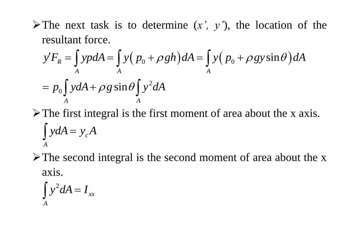
The next task is to determine (x’, y’), the location of the
resultant force.
0 0
2
0
sin
sin
R
A A A
A A
y F ypdA y p gh dA y p gy dA
p ydA g y dA
The first integral is the first moment of area about the x axis.
c
A
ydA y A
The second integral is the second moment of area about the x
axis. 2
xx
A
y dA I
We can use the parallel axis theorem, 2
ˆˆxx xx cI I Ay , to
replace Ixx with the standard second moment of area, about
the centroidal x̂ axis.
2 2
ˆ ˆ0 0
ˆ ˆ0
ˆ ˆ ˆ ˆ0
sin sin
sin sin
sin sin
R c xx c
A A
c c xx
c c xx c R xx
y F p ydA g y dA p y A g I Ay
y p gy A g I
y p gh A g I y F g I
ˆˆsin xxc
R
g Iy y
F
If we have the same ambient pressure acting on the other side
of the surface, then
ˆ ˆ
singageR c c
xxc
c
F p A gy A
Iy y
Ay
Note that in any event, y’>yc—the location of the force is
always below the level of the plate centroid. This makes
sense, the pressures will always be larger on the lower
regions, moving the resultant force down the plate.
A similar analysis can be done to compute x’, the x location
of the force on the plate.
0 0
0
sin
sin
R
A A A
A A
x F xpdA x p gh dA x p gy dA
p xdA g xydA
The first integral is the first moment of area about the y axis.
c
A
xdA x A
The second integral is the second moment of area about the x
axis.
xy
A
xydA I
Using the parallel axis theorem, ˆˆxy xy c cI I Ax y , we find
ˆˆ0 0
ˆˆ0
ˆˆ ˆˆ0
sin sin
sin sin
sin sin
R c xy c c
A A
c c xy
c c xy c R xy
x F p xdA g xydA p x A g I Ax y
x p gy A g I
x p gh A g I x F g I
ˆˆsin xy
c
R
g Ix x
F
In summary, above equations constitute a complete set of
equations for computing the magnitude and location of the
force due to hydrostatic pressure on any submerged plane
surface.
The direction of the force will always be perpendicular to the
plane. We can now consider several examples using these
equations. In Example 3.5 we use both the integral and
algebraic sets of equations.
Centroids of areas:
The location of the centroid of a plane area is an important
geometric property of the area.
To define the coordinates of the centroid, let us refer to the
area A and the xy coordinates system shown. In addition, the
first moments of the area about the x and y axes, respectively,
are
, ,x yQ ydA Q xdA
The coordinates x and y of the centroid C are equal to the
first moments divided by the area itself:
, y x
xdA ydAQ Qx y
A AdA dA
Moments of inertia of areas:
The momentum of inertia of a plane area with respect to the x
and y axes, respectively, are defined by the integrals 2 2, x yI y dA I x dA
in which x and y are the coordinates of the differential
element of area dA. Because dA is multiplied by the square of
the distance, moments of inertia are also called second
moments of the area.
Note that the moment of inertia is different with respect to
different axis. In general, the moment of inertia increases as
the reference axis is moved parallel to itself farther from the
centroid.
Parallel-Axis theorem for moments of inertia
The moment of inertia of an area with respect to any axis in
the plane of the area is related to the moment of inertia with
respect to a parallel centroidal axis by the parallel-axis
theorem.
2
2 2
1 1 1
2
1
2
where 0c
x
x x
I y d dA y dA d ydA d dA
I I Ad ydA
The first integral on the right-hand side is the moment of
inertia cxI with respect to the xc axis; the second integral
vanishes because the xc axis passes through the centroid; and
the third integral is the area A of the figure.
Proceeding in the same manner for the y axis, we obtain 2
2 cy yI I Ad
The parallel-axis theorem for moments of inertia: The
moment of inertia with respect to a parallel centroidal axis
plus the product of the area and the square of the distance
between the two axes.
Products of inertia
The product of inertia of a plane area is a property that is
defined with respect to a set of perpendicular axes lying in the
plane of the area. We define the product of inertia with
respect to the x and y axes as follows:
xyI xydA
The product of inertia of an area is zero with respect to any
pair axes in which one axis is an axis of symmetry.
The products of inertia of an area with respect to parallel sets
of axes are related by a parallel-axis theorem that is
analogous to the corresponding theorems for moments of
inertia.
2 1 1 2 1 2
1 2d where 0, 0c c
xy
xy x y
I x d y d dA xydA d xdA d ydA d d dA
I I Ad xdA ydA
The parallel-axis theorem for products of inertia: the
product of inertia of an area with respect to any pair of axes
in its plane is equal to the product of inertia with respect to
parallel centroidal axes plus the product of the area and the
coordinates of the centroid with respect to the pair of axes.
Ex. 3.5 Resultant Force on Inclined Plane Submerged Surface:
The inclined surface shown, hinged along edge A, is 5 m wide.
Determine the resultant force, FR, of the water and the air on the
inclined surface.
Given: Rectangular gate, hinged along A, w=5 m.
Find: Resultant force, FR, of the water and the air on the gate.
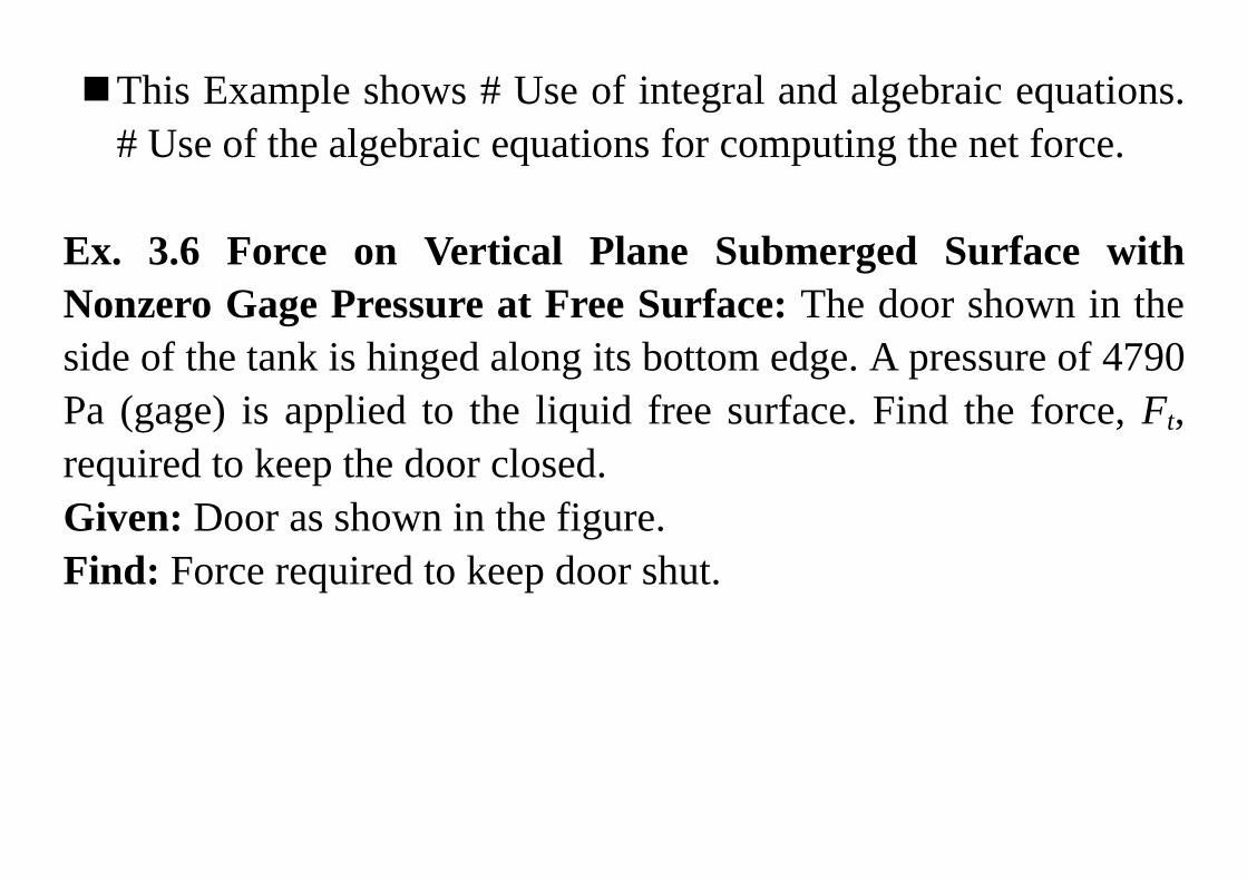
This Example shows # Use of integral and algebraic equations.
# Use of the algebraic equations for computing the net force.
Ex. 3.6 Force on Vertical Plane Submerged Surface with
Nonzero Gage Pressure at Free Surface: The door shown in the
side of the tank is hinged along its bottom edge. A pressure of 4790
Pa (gage) is applied to the liquid free surface. Find the force, Ft,
required to keep the door closed.
Given: Door as shown in the figure.
Find: Force required to keep door shut.
This Example shows:# Use of algebraic equations for nonzero
gage pressure at the liquid free surface. # Use of the moment
equation from statics for computing the required applied force.
Hydrostatic Force on a Curved Submerged Surface
Unlike for the plane surface, we have a more complicated
problem—the pressure force is normal to the surface at each
point, but now the infinitesimal area elements point in
varying directions because of the surface curvature.
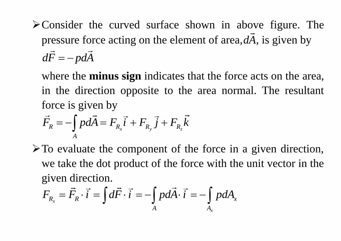
Consider the curved surface shown in above figure. The
pressure force acting on the element of area,dA, is given by
dF pdA
where the minus sign indicates that the force acts on the area,
in the direction opposite to the area normal. The resultant
force is given by
x y zR R R R
A
F pdA F i F j F k
To evaluate the component of the force in a given direction,
we take the dot product of the force with the unit vector in the
given direction.
x
x
R R x
A A
F F i dF i pdA i pdA
Since, in any problem, the direction of the force component
can be determined by inspection, the use of vectors is not
necessary. In general, the magnitude of the component of the
resultant force in the l direction is given by
l
l
R l
A
F pdA
We have the interesting result that the horizontal force and
its location are the same as for an imaginary vertical
plane surface of the same projected area.
xR H x cF F pdA p A
With atmospheric pressure at the free surface and on the other
side of the curved surface the net vertical force will be
equal to the weight of fluid directly above the surface.
zR V z zF F pdA ghdA gdV gV
In summary, for a curved surface we can use two simple
formulas for computing the horizontal and vertical force
components due to the fluid only (no ambient pressure),
, H c VF p A F gV
It can be shown that the line of action of the vertical force
component passes through the center of gravity of the volume
of liquid directly above the curved surface.
Ex. 3.7 Force Components on a Curved Submerged Surface:
The gate shown is hinged at O and has constant width, w=5 m. The
equation of the surface is x=y2/a, where a=4 m. The depth of water
to the right of the gate is D=4 m. Find the magnitude of the force,
Fa, applied as shown, required to maintain the gate in equilibrium
if the weight of the gate is neglected.
Given: Gate of constant width, w=5 m. Equation of surface in xy
plane is x=y2/a, where a=4 m. Water stands at depth D=4 m to the
right of the gate. Force Fa is applied as shown, and weight of gate
is to be neglected. (Note that for simplicity we do not show the
reactions at O.)
Find: Force Fa required to maintain the gate in equilibrium.
This Example shows: # Use of vertical flat plate equations for
the horizontal force, and fluid weight equations for the vertical
force, on a curved surface. # The use of “thought experiments”
to convert a problem with fluid below a curved surface into an
equivalent problem with fluid above.
3.6 Buoyancy and Stability
If an object is immersed in a liquid, or floating on its surface,
the net vertical force acting on it due to liquid pressure is
termed buoyancy.
The vertical force on the body due to hydrostatic pressure may
be found most easily by considering cylindrical volume
elements similar to the one shown in the above figure.
0 2 0 1
2 1
z zF dF p gh dA p gh dA
g h h dA gV
Hence we conclude that for a submerged body the buoyancy
force of the fluid is equal to the weight of displaced fluid,
buoyancyF gV
This relation reportedly was used by Archimedes in 220 B.C. to
determine the gold content in the crown of King Hiero II.
Consequently, it is often called “Archimedes’ Principle.”
In cases of partial immersion, a floating body displaces its
own weight of the liquid in which it floats.
Ex. 3.8 Buoyancy Force in a Hot Air Balloon: A hot air balloon
(approximated as a sphere of diameter 15 m) is to lift a basket load
of 2670 N. To what temperature must the air be heated in order to
achieve liftoff?
Given: Atmosphere at STP, diameter of balloon d = 15 m, and load
Wload = 2670 N.
Find: The hot air temperature to attain liftoff.
Notes: # Absolute pressures and temperatures are always used
in the ideal gas equation. # This problem demonstrates that for
lighter-than-air vehicles the buoyancy force exceeds the vehicle
weight—that is, the weight of fluid (air) displaced exceeds the
vehicle weight.
The line of action of the buoyancy force acts through the
centroid of the displaced volume. Since floating bodies are in
equilibrium under body and buoyancy forces, the location of the
line of action of the buoyancy force determines stability.
The weight of an object acts through its center of gravity, CG,
the lines of action of the buoyancy and the weight are offset in
such a way as to produce a couple that tends to right the craft.
In above right figure, the couple tends to capsize the craft.
Ballast may be needed to achieve roll stability. Wooden
warships carried stone ballast low in the hull to offset the
weight of the heavy cannon on upper gun decks.
3.7 Fluids in Rigid-Body Motion
This section is omitted.
3.8 Summary and Useful Equations
In this chapter we have reviewed the basic concepts of fluid
statics. This included:
Deriving the basic equation of fluid statics in vector form.
Applying this equation to compute the pressure variation in a
static fluid:
Incompressible liquids: pressure increases uniformly with
depth.
Gases: pressure decreases nonuniformly with elevation
(dependent on other thermodynamic properties).
Study of:
Gage and absolute pressure.
Use of manometers and barometers.
Analysis of the fluid force magnitude and location on
submerged:
Plane surfaces.
Curved surfaces.
Derivation and use of Archimedes’ Principle of Buoyancy.