Outline of the PresentationOutline of the Presentation
3.1 Introduction to Inventory Management 3.2 Single Warehouse Inventory
(1) EOQ (2) Demand Forecast (3) Supply Contracts (4) A multi-Period Inventory Model (5) Periodic Review Policy
3.3 Risk Pooling 3.4 Centralized vs. Decentralized Systems 3.5 Managing Inventory in the SC 3.6 Practical Issues in Inventory Management
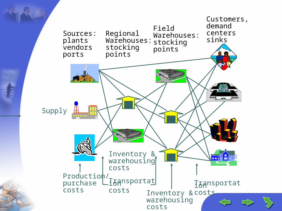
Supply
Sources:plantsvendorsports
RegionalWarehouses:stocking points
Field Warehouses:stockingpoints
Customers,demandcenterssinks
Production/purchase costs
Inventory &warehousing costs
Transportation costs Inventory &
warehousing costs
Transportation costs
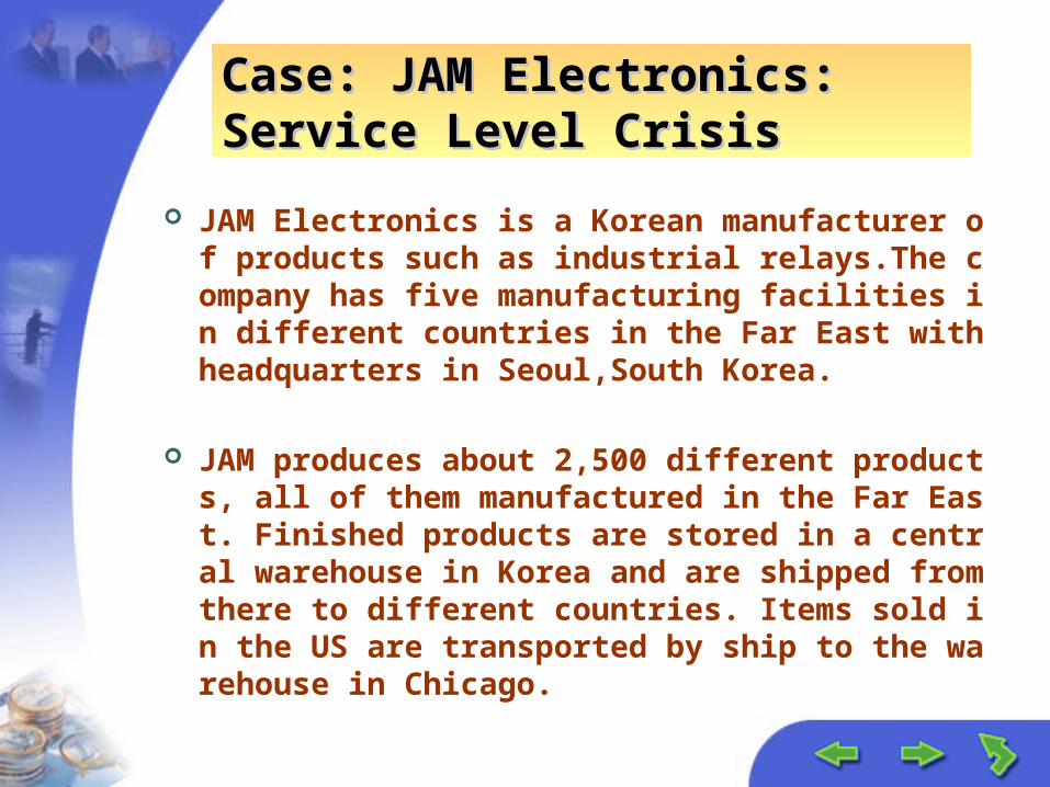
Case: JAM Electronics: Service Case: JAM Electronics: Service Level CrisisLevel Crisis
JAM Electronics is a Korean manufacturer of products such as industrial relays.The company has five manufacturing facilities in different countries in the Far East with headquarters in Seoul,South Korea.
JAM produces about 2,500 different products, all of them manufactured in the Far East. Finished products are stored in a central warehouse in Korea and are shipped from there to different countries. Items sold in the US are transported by ship to the warehouse in Chicago.
Case: JAM ElectronicsCase: JAM Electronics
Problems: the service level is at an all-time low. Only about 70% of all orders are delivered on time. Difficulty forecasting customer demand. Long lead time in the supply chain. The large number of SKUs handled by JAM USA.
Case: JAM ElectronicsCase: JAM Electronics
0
50
100
150
200
250
Demand (Inthousands)
Apr MayJuneJul yAugSep. Oct NovDec JanFebMar
Months
Monthl y Demand for i tem xxx-1534
By the end of this chapter, you should be able to understand the following issues:
How a firm can cope with huge variability in customer demand.
What the relationship is between service and inventory levels.
What an effective inventory management policy is.
4.1 Inventory4.1 Inventory
Where do we hold inventory? Suppliers and manufacturers warehouses and distribution centers retailers
Types of Inventory WIP raw materials finished goods
Why do we hold inventory? Economies of scale Uncertainty in supply and demand Lead Time, Capacity limitations
Goals: Goals: Reduce Cost, Improve ServiceReduce Cost, Improve Service
By effectively managing inventory: Xerox eliminated $700 million inventory from its
supply chain Wal-Mart became the largest retail company
utilizing efficient inventory management GM has reduced parts inventory and
transportation costs by 26% annually
Goals: Goals: Reduce Cost, Improve ServiceReduce Cost, Improve Service
By not managing inventory successfully In 1994, “IBM continues to struggle with shortages in their
ThinkPad line” (WSJ, Oct 7, 1994) In 1993, “Liz Claiborne said its unexpected earning decline
is the consequence of higher than anticipated excess inventory” (WSJ, July 15, 1993)
In 1993, “Dell Computers predicts a loss; Stock plunges. Dell acknowledged that the company was sharply off in its forecast of demand, resulting in inventory write downs” (WSJ, August 1993)
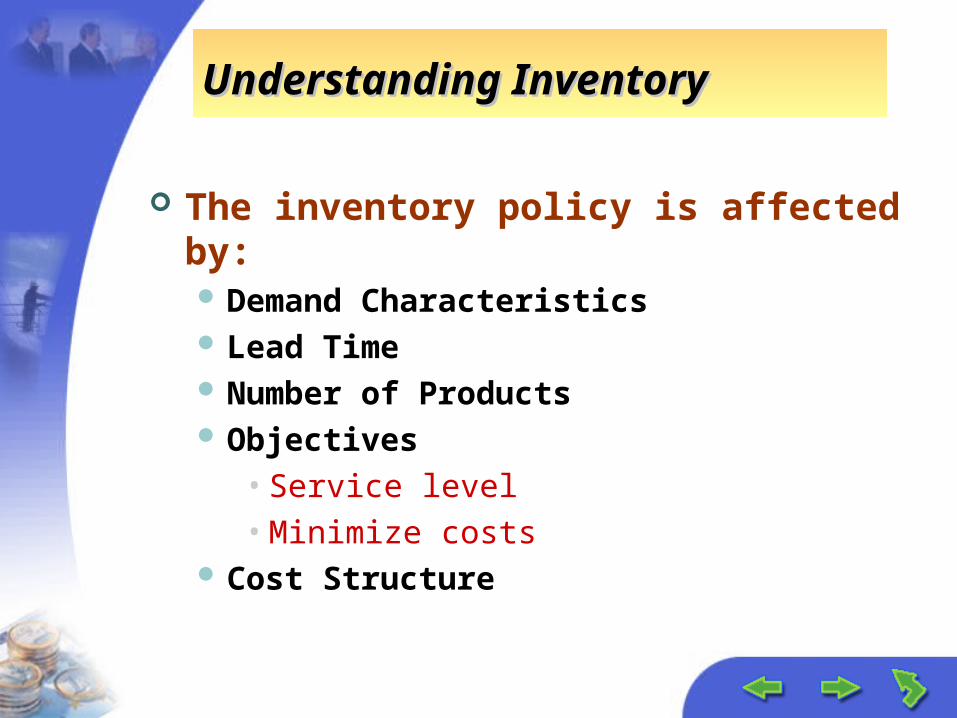
Understanding InventoryUnderstanding Inventory
The inventory policy is affected by: Demand Characteristics Lead Time Number of Products Objectives
• Service level
• Minimize costs Cost Structure
Cost StructureCost Structure
Order costs Fixed Variable
Holding Costs Insurance Maintenance and Handling Taxes Opportunity Costs Obsolescence
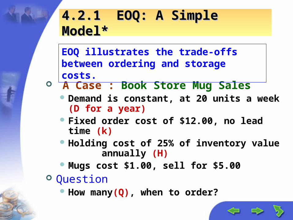
4.2.1 EOQ: A Simple Model*4.2.1 EOQ: A Simple Model*
A Case : Book Store Mug Sales Demand is constant, at 20 units a week (D for a
year) Fixed order cost of $12.00, no lead time (k) Holding cost of 25% of inventory value
annually (H) Mugs cost $1.00, sell for $5.00
Question How many(Q), when to order?
EOQ illustrates the trade-offs between ordering and storage costs.
EOQ: A View of Inventory*EOQ: A View of Inventory*
Time
Inventory
OrderSize
Note:• No Stockouts• Order when no inventory• Order Size determines policy
Avg. Inven
EOQ: Calculating Total Cost*EOQ: Calculating Total Cost*
Purchase Cost Constant Holding Cost: (Avg. Inven) * (Holding Cost) Ordering (Setup Cost):Number of Orders * Order Cost
Goal: Find the Order Quantity that Minimizes These Costs
EOQ:Total Cost*EOQ:Total Cost*
0
20
40
60
80
100
120
140
160
0 500 1000 1500
Order Quantity
Co
st
Total Cost
Order Cost
Holding Cost
EOQ: Optimal Order Quantity*EOQ: Optimal Order Quantity*
Find order quantity that maximizes weighted average profit.
Question: Will this quantity be less than, equal to, or greater than average demand?
What to Make?What to Make?
Question: Will this quantity be less than, equal to, or greater than average demand?
Average demand is 13,100 Look at marginal cost Vs. marginal profit
if extra jacket sold, profit is 125-80 = 45 if not sold, cost is 80-20 = 60
So we will make less than average
SnowTime Expected ProfitSnowTime Expected Profit
Expected Profit
$0
$100,000
$200,000
$300,000
$400,000
8000 12000 16000 20000
Order Quantity
Pro
fit
The quantity that maximizes average profit, is about 12,000.
SnowTime Expected ProfitSnowTime Expected Profit
Expected Profit
$0
$100,000
$200,000
$300,000
$400,000
8000 12000 16000 20000
Order Quantity
Pro
fit
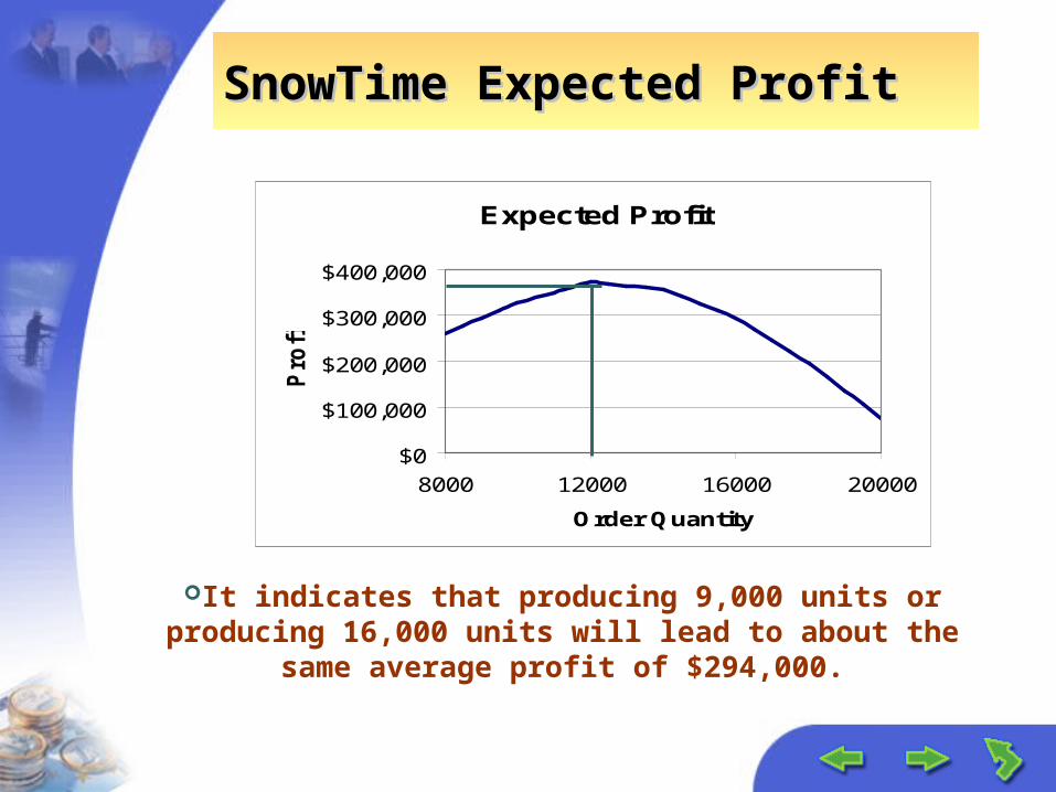
It indicates that producing 9,000 units or producing 16,000 units will lead to about the same average profit of $294,000.
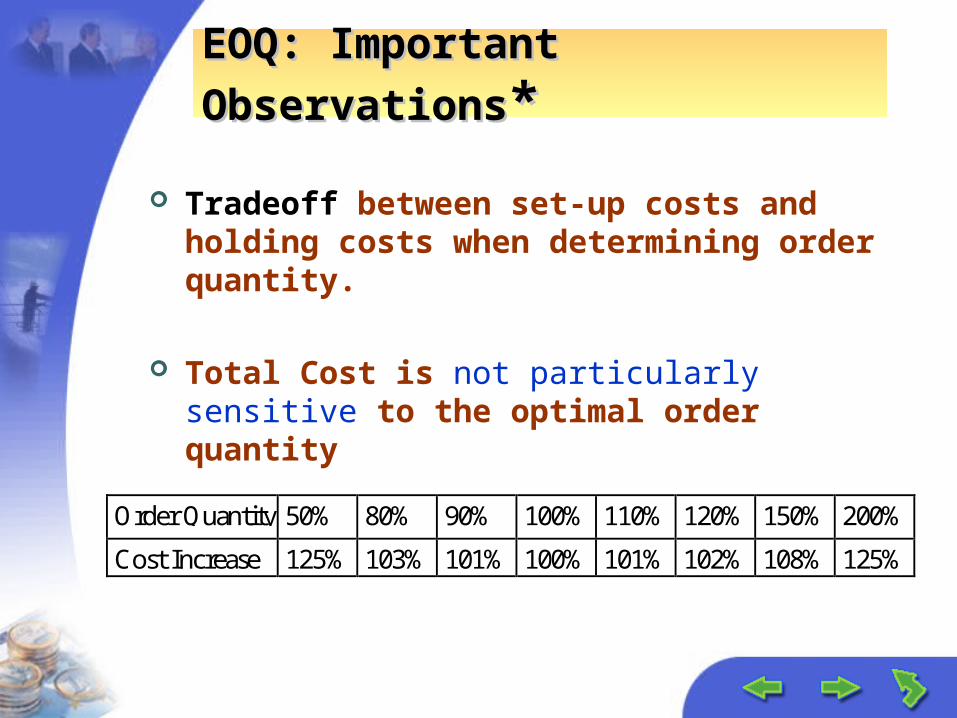
SnowTime:SnowTime: Important ObservationsImportant Observations
Tradeoff between ordering enough to meet demand and ordering too much
Several quantities have the same average profit Average profit does not tell the whole story
Question: 9000 and 16000 units lead to about the same average profit, so which do we prefer?
SnowTime Expected ProfitSnowTime Expected Profit
Expected Profit
$0
$100,000
$200,000
$300,000
$400,000
8000 12000 16000 20000
Order Quantity
Pro
fit
Probability of OutcomesProbability of Outcomes
0%
20%
40%
60%
80%
100%
Revenue
Pro
ba
bilit
y
Q=9000
Q=16000
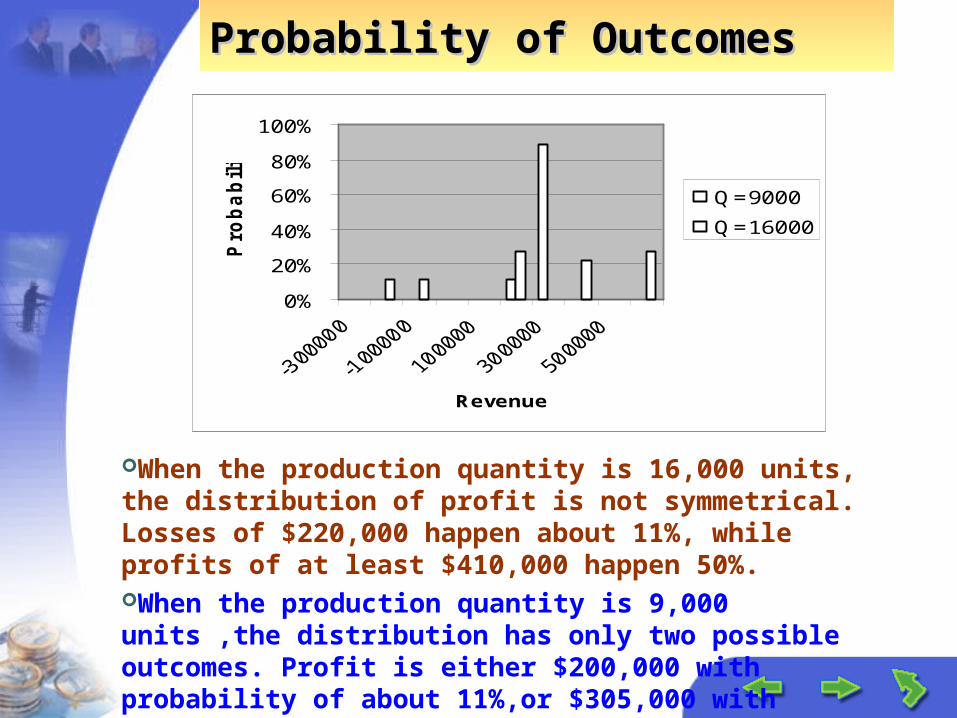
When the production quantity is 16,000 units, the distribution of profit is not symmetrical. Losses of $220,000 happen about 11%, while profits of at least $410,000 happen 50%. When the production quantity is 9,000 units ,the distribution has only two possible outcomes. Profit is either $200,000 with probability of about 11%,or $305,000 with probability of about 89%.
Key Insights from this ModelKey Insights from this Model
The optimal order quantity is not necessarily equal to average forecast demand
The optimal quantity depends on the relationship between marginal profit and marginal cost
As order quantity increases, average profit first increases and then decreases
As production quantity increases, risk increases. In other words, the probability of large gains and of large losses increases
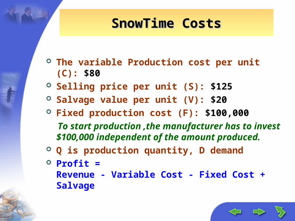
SnowTime Costs: The Effect of IniSnowTime Costs: The Effect of Initial Inventory tial Inventory
Production cost per unit (C): $80 Selling price per unit (S): $125 Salvage value per unit (V): $20 Fixed production cost (F): $100,000 Q is production quantity, D demand
Suppose that one of the jacket designs is a model produced last year.
Some inventory is left from last year Assume the same demand pattern as before If only old inventory is sold, no setup cost
Question: If there are 5000 units remaining, what should SnowTime do? What should they do if there are 10,000 remaining?
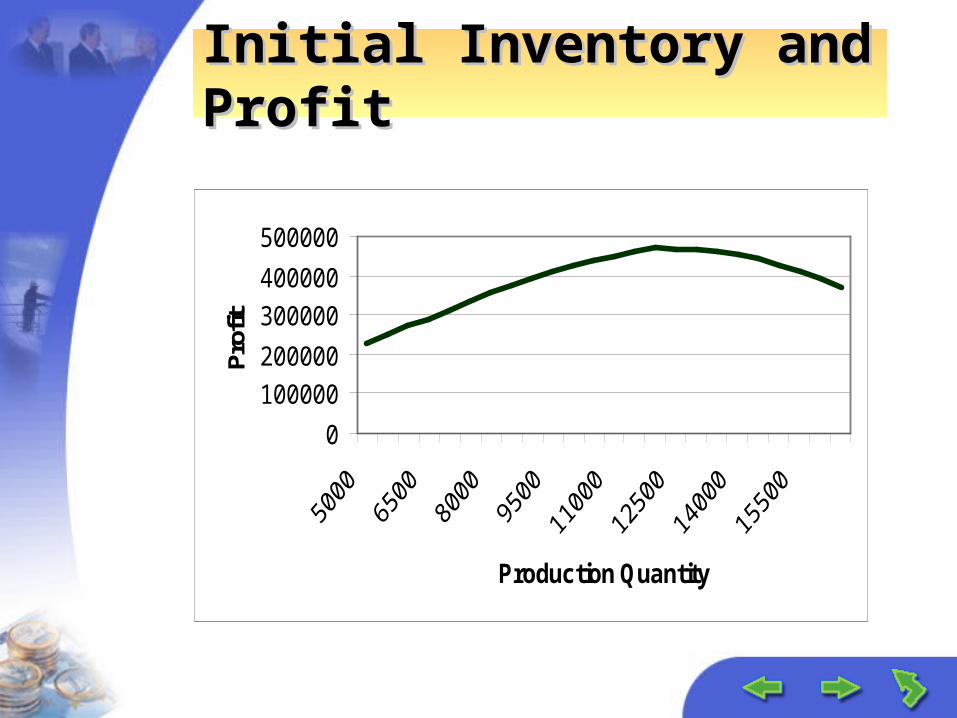
Initial Inventory and ProfitInitial Inventory and Profit
0
100000
200000
300000
400000
500000
Production Quantity
Pro
fit
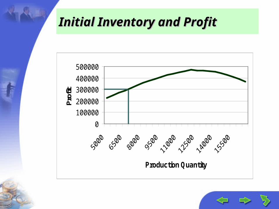
Initial Inventory and ProfitInitial Inventory and Profit
0
100000
200000
300000
400000
500000
Production Quantity
Pro
fit
Initial Inventory and ProfitInitial Inventory and Profit
0
100000
200000
300000
400000
500000
Production Quantity
Pro
fit
If the manufacturer does not produce any additional suits, no more than 5,000 units can be sold and no additional fixed cost will be incurred. However, it the manufacturer decides to produce, a fixed production cost is charged independent of the amount produced.
Initial Inventory and ProfitInitial Inventory and Profit
0
100000
200000
300000
400000
500000
50
00
60
00
70
00
80
00
90
00
10
00
0
11
00
0
12
00
0
13
00
0
14
00
0
15
00
0
16
00
0
Production Quantity
Pro
fit
Average profit excluding fixed production cost
Average profit including fixed production cost
(1) there are 5000 units remaining If nothing is produced, average profit is equal to 625000. Production should increase inventory from 5,000 units to 12,000
units. Thus, average profit is equal to 771000 (from the figure). (2) there are 10,000 units remaining It is easy to see that there is no need to produce anything becaus
e the average profit associated with an initial inventory of 10,000 is larger than what we would achieve if we produce to increase inventory to 12,000 units.
If we produce, the most we can make on average is a profit of$375,000. This is the same average profit that we will have if our initial inventory is about 8,500 units.
Hence, if our initial inventory is below 8,5000 units, we produce to raise the inventory level to 12,000 units. If initial inventory is at least 8,5000 units,we should not produce anything.
Analysis Analysis
(s, S) Policies(s, S) Policies
For some starting inventory levels, it is better to not start production
If we start, we always produce to the same level Thus, we use an (s,S) policy. If the inventory
level is below s, we produce up to S. s is the reorder point, and S is the order-up-to
level The difference between the two levels is driven
by the fixed costs associated with ordering, transportation, or manufacturing
Manufacturer Manufacturer DC Retail DC
Stores
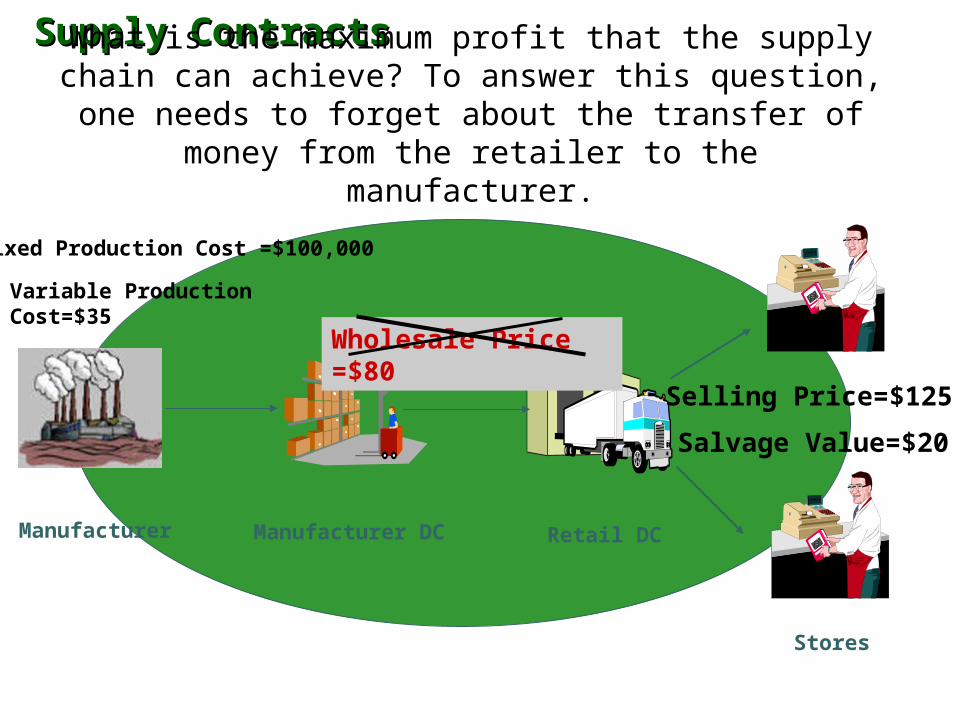
Fixed Production Cost =$100,000
Variable Production Cost=$35
Selling Price=$125
Salvage Value=$20
Wholesale Price =$80
4.2.3 Supply Contracts4.2.3 Supply Contracts
Who takes the risk? What would the manufacturer like?
Distributor optimal order quantity is 12,000 units
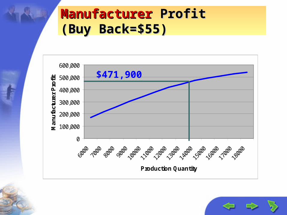
Distributor expected profit is $470,000 Manufacturer profit is $440,000 Supply Chain Profit is $910,000
–Is there anything that the distributor and manufacturer can do to increase the profit of both?
Manufacturer Manufacturer DC Retail DC
Stores
Fixed Production Cost =$100,000
Variable Production Cost=$35
Selling Price=$125
Salvage Value=$20
Wholesale Price =$80
Supply Contracts Supply Contracts (between manufacturer and retailer)(between manufacturer and retailer)
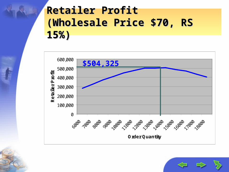
In the previous strategy, the retailer takes all the risk and the manufacturer takes zero risk. This is why the retailer has to be very conservative with the amount he orders.
If the retailer can transfer some of the risk to the manufacturer, the retailer may be willing to increase his order quantity and thus increase both his profit and the manufacturer profit.
Supply ContractsSupply ContractsWhat is the maximum profit that the supply chain can achieve? To answer this question, one needs to forget about the transfer
Effective supply contracts allow supply chain partners to replace sequential optimization by global optimization
Buy Back and Revenue Sharing contracts achieve this objective through risk sharing
Supply Contracts: Case StudySupply Contracts: Case Study
Example: Demand for a movie newly released video cassette typically starts high and decreases rapidly Peak demand last about 10 weeks
Blockbuster purchases a copy from a studio for $65 and rent for $3 Hence, retailer must rent the tape at least 22 times
before earning profit Retailers cannot justify purchasing enough to
cover the peak demand In 1998, 20% of surveyed customers reported that
they could not rent the movie they wanted
Supply Contracts: Case StudySupply Contracts: Case Study
Starting in 1998 Blockbuster entered a revenue sharing agreement with the major studios Studio charges $8 per copy Blockbuster pays 30-45% of its rental income
Even if Blockbuster keeps only half of the rental income, the breakeven point is 6 rental per copy
The impact of revenue sharing on Blockbuster was dramatic Rentals increased by 75% in test markets Market share increased from 25% to 31% (The 2nd largest
retailer, Hollywood Entertainment Corp has 5% market share)
Other ContractsOther Contracts
Quantity Flexibility Contracts Supplier provides full refund for returned items
as long as the number of returns is no larger than a certain quantity
Sales Rebate Contracts Supplier provides direct incentive for the retailer
to increase sales by means of a rebate paid by the supplier for any item sold above a certain quantity
4.2.4 A Multi-Period Inventory Model4.2.4 A Multi-Period Inventory Model
Often, there are multiple reorder opportunities
Consider a central distribution facility which orders from a manufacturer and delivers to retailers. The distributor periodically places orders to replenish its inventory
The DC holds inventory to:The DC holds inventory to:
Satisfy demand during lead time Protect against demand uncertainty Balance fixed costs and holding costs
Reminder:Reminder: The Normal DistributionThe Normal Distribution
0 10 20 30 40 50 60
Average = 30
Standard Deviation = 5
Standard Deviation = 10
The Multi-Period Continuous Review The Multi-Period Continuous Review Inventory ModelInventory Model
Normally distributed random demand Fixed order cost plus a cost proportional to
amount ordered. Inventory cost is charged per item per unit time If an order arrives and there is no inventory, the
order is lost The distributor has a required service level.
This is expressed as the the likelihood that the distributor will not stock out during lead time.
Intuitively, how will this effect our policy?
A View of (s, S) PolicyA View of (s, S) Policy
Time
Inve
ntor
y L
evel
S
s
0
LeadTimeLeadTime
Inventory Position
The (s,S) PolicyThe (s,S) Policy
(s, S) Policy: Whenever the inventory position drops below a certain level, s, we order to raise the inventory position to level S.
The reorder point is a function of: The Lead Time Average demand Demand variability Service level
NotationNotation
AVG = average daily demand STD = standard deviation of daily demand LT = replenishment lead time in days h = holding cost of one unit for one day K = fixed cost SL = service level (for example, 95%). This implies that
the probability of stocking out is 100%-SL (for example, 5%)
Also, the Inventory Position at any time is the actual inventory plus items already ordered, but not yet delivered.
AnalysisAnalysis
The reorder point (s) has two components: To account for average demand during lead time:
LTAVG To account for deviations from average (we call this safety
stock)
z STD LT
where z is chosen from statistical tables to ensure that the probability of stockouts during leadtime is 100%-SL.
Since there is a fixed cost, we order more than up to the reorder point:
Q=(2 K AVG)/h The total order-up-to level is:
S=Q+s
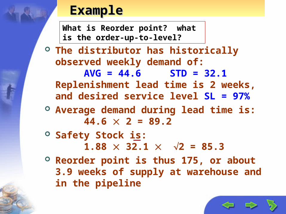
ExampleExample
The distributor has historically observed weekly demand of:
AVG = 44.6 STD = 32.1Replenishment lead time is 2 weeks, and desired service level SL = 97%
Average demand during lead time is:44.6 2 = 89.2
Safety Stock is:1.88 32.1 2 = 85.3
Reorder point is thus 175, or about 3.9 weeks of supply at warehouse and in the pipeline
What is Reorder point? what is the order-up-to-level?
Each review echelon, inventory position is raised to the base-stock level.
The base-stock level includes two components: Average demand during r+L days (the time until
the next order arrives):(r+L)*AVG
Safety stock during that time:z*STD* r+L
4.3 Risk Pooling Example4.3 Risk Pooling Example
Consider these two systems: Some problems faced by ACME, a company that
produces and distributes electronic equipment in the Northeast of the United States.
(1)The current distribution system partitions the Northeast into two markets, each of which has a single warehouse. Retailers receive items directly from the warehouses; each retailer is assigned to a single market and receives deliveries from the corresponding warehouse.
Supplier
Warehouse One
Warehouse Two
Market One
Market Two
Risk Pooling Example (cont’)Risk Pooling Example (cont’)
(2)Replace the two warehouses with a single warehouse. The same service level,97%, be maintained regardless of the logistics strategy employed.
This system allows ACME to achieve either the same service level of 97% with much lower inventory or a higher service level with the same amount of total inventory.
Market Two
Supplier Warehouse
Market One
Risk Pooling Example (cont’)Risk Pooling Example (cont’)
For the same service level, which system will require more inventory? Why?
For the same total inventory level, which system will have better service? Why?
What are the factors that affect these answers?
Risk Pooling Example (cont’)Risk Pooling Example (cont’)
Compare the two systems:two products(A,B)maintain 97% service level$60 order cost$.27 weekly holding cost$1.05 transportation cost per unit in
decentralized system, $1.10 in centralized system
1 week lead time
Table 1 Historical Data for Product A and B
Risk Pooling ExampleRisk Pooling Example
Week 1 2 3 4 5 6 7 8
Prod A,Market 1
33 45 37 38 55 30 18 58
Prod A,Market 2
46 35 41 40 26 48 18 55
Prod B,Market 1
0 2 3 0 0 1 3 0
Product B,Market 2
2 4 0 0 3 1 0 0
The tables include weekly demand information for each product for the last eight weeks in each market area. Observe that Product B is a slow-moving product –the demand for Product B is fairly small relative to the demand for Product A.
Risk Pooling:Risk Pooling:Types of Risk Pooling*Types of Risk Pooling*
Risk Pooling Across Markets Risk Pooling Across Products Risk Pooling Across Time
Daily order up to quantity is:• LTAVG + z AVG LT
10 1211 13 14 15
Demands
Orders
4.4 To Centralize or not to 4.4 To Centralize or not to CentralizeCentralize
What are the trade-offs that we need to consider in comparing centralized distribution systems with decentralized distribution systems?
What is the effect on: Safety stock? Service level? Overhead? Lead time? Transportation Costs?
Centralized vs Decentralized Centralized vs Decentralized systemsystem
Safety stock. Clearly, safety stock decreases as a firm moves from a decentralized to a centralized system.
Service level. When the centralized and decentralized systems have the same total safety stock, the service level provided by the centralized system is higher.
Lead time. Since the warehouses are much closer to the customers in a decentralized system,response time is much lower.
The warehouse echelon inventory
Supplier
Warehouse
Retailers
4.5 Managing Inventory in the SC 4.5 Managing Inventory in the SC (Centralized Systems*)(Centralized Systems*)
The warehouse policy The warehouse policy controls its echelon controls its echelon inventory position, that inventory position, that is, whenever the is, whenever the echelon inventory echelon inventory position for the W is position for the W is below s, an order is below s, an order is placed to raise its placed to raise its echelon inventory echelon inventory position to S.position to S.
Centralized Distribution Centralized Distribution Systems*Systems*
Question: How much inventory should management keep at each location?
A good strategy: The retailer raises inventory to level Sr each period
The supplier raises the sum of inventory in the retailer and supplier warehouses and in transit to Ss
If there is not enough inventory in the warehouse to meet all demands from retailers, it is allocated so that the service level at each of the retailers will be equal.
4.6 Inventory Management: 4.6 Inventory Management: Best PracticeBest Practice
Periodic inventory reviews Tight management of usage rates, lead
times and safety stock ABC approach Reduced safety stock levels Shift more inventory, or inventory
ownership, to suppliers Quantitative approaches
Changes In Inventory TurnoverChanges In Inventory Turnover
Inventory turnover ratio = annual sales/avg. inventory level
Inventory turns increased by 30% from 1995 to 1998
Inventory turns increased by 27% from 1998 to 2000
Overall the increase is from 8.0 turns per year to over 13 per year over a five year period ending in year 2000.
Industry Upper Quartile
Median Lower Quartile
Dairy Products 34.4 19.3 9.2
Electronic Component 9.8 5.7 3.7
Electronic Computers 9.4 5.3 3.5
Books: publishing 9.8 2.4 1.3
Household audio & video equipment
6.2 3.4 2.3
Household electrical appliances
8.0 5.0 3.8
Industrial chemical 10.3 6.6 4.4
Inventory Turnover RatioInventory Turnover Ratio
Factors that Drive Reduction in Factors that Drive Reduction in
InventoryInventory
Top management emphasis on inventory reduction (19%)
Reduce the Number of SKUs in the warehouse (10%)
Improved forecasting (7%) Use of sophisticated inventory management
software (6%) Coordination among supply chain members
(6%) Others
Factors that Drive Inventory Factors that Drive Inventory Turns IncreaseTurns Increase
Better software for inventory management (16.2%)
Reduced lead time (15%) Improved forecasting (10.7%) Application of SCM principals (9.6%) More attention to inventory management (6.6%) Reduction in SKU (5.1%) Others
ForecastingForecasting
Recall the three rules Nevertheless, forecast is critical General Overview:
Judgment methods Market research methods Time Series methods Causal methods
Judgment MethodsJudgment Methods
Assemble the opinion of experts Sales-force composite combines
salespeople’s estimates Panels of experts – internal, external,
both Delphi method
Each member surveyed Opinions are compiled Each member is given the opportunity to change
his opinion
Market Research MethodsMarket Research Methods
Particularly valuable for developing forecasts of newly introduced products
Market testing Focus groups assembled. Responses tested. Extrapolations to rest of market made.
Market surveys Data gathered from potential customers Interviews, phone-surveys, written surveys, etc.
Time Series MethodsTime Series Methods Past data is used to estimate future data Examples include
Moving averages – average of some previous demand points.
Exponential Smoothing – more recent points receive more weight
Methods for data with trends:• Regression analysis – fits line to data• Holt’s method – combines exponential smoothing concepts
with the ability to follow a trend Methods for data with seasonality
• Seasonal decomposition methods (seasonal patterns removed)• Winter’s method: advanced approach based on exponential smoothing
Complex methods (not clear that these work better)
Causal MethodsCausal Methods
Forecasts are generated based on data other than the data being predicted
Examples include: Inflation rates GNP Unemployment rates Weather Sales of other products
Selecting the Appropriate Selecting the Appropriate Approach:Approach:
What is the purpose of the forecast? Gross or detailed estimates?
What are the dynamics of the system being forecast? Is it sensitive to economic data? Is it seasonal? Trending?
How important is the past in estimating the future? Different approaches may be appropriate for different
stages of the product lifecycle: Testing and intro: market research methods, judgment methods Rapid growth: time series methods Mature: time series, causal methods (particularly for long-range
planning) It is typically effective to combine approaches.